Accuracy of Simulated Diurnal Valley Winds in the Swiss Alps: Influence of Grid Resolution, Topography Filtering, and Land Surface Datasets


1
Institute for Atmospheric and Environmental Sciences, Goethe University Frankfurt, 60438 Frankfurt, Germany
2
Institute for Atmospheric and Climate Science, ETH Zurich, 8092 Zurich, Switzerland
3
Institute for Climate and Atmospheric Science, University of Leeds, Leeds LS2 9JT, UK
4
Federal Institute of Meteorology and Climatology, MeteoSwiss, 8058 Zurich-Flughafen, Switzerland
*
Author to whom correspondence should be addressed.
Atmosphere 2018, 9(5), 196; https://doi.org/10.3390/atmos9050196
Submission received: 23 February 2018
/
Revised: 6 May 2018
/
Accepted: 15 May 2018
/
Published: 18 May 2018
(This article belongs to the Special Issue Atmospheric Processes over Complex Terrain)
Abstract
:We evaluate the near-surface representation of thermally driven winds in the Swiss Alps in a numerical weather prediction model at km-scale resolution. In addition, the influence of grid resolution (2.2 km and 1.1 km), topography filtering, and land surface datasets on the accuracy of the simulated valley winds is investigated. The simulations are evaluated against a comprehensive set of surface observations for an 18-day fair-weather summer period in July 2006. The episode is characterized by strong diurnal wind systems and the formation of shallow convection over the mountains, which transitions to precipitating convection in some areas. The near-surface winds (10 m above ground level) follow a typical diurnal pattern with strong daytime up-valley flow and weaker nighttime down-valley flow. At a 2.2 km resolution the valley winds are poorly simulated for most stations, while at a 1.1 km resolution the diurnal cycle of the valley winds is well represented in most large (e.g., Rhein valley at Chur and Rhone valley at Visp) and medium-sized valleys (e.g., Linth valley at Glarus). In the smaller valleys (e.g., Maggia valley at Cevio), the amplitude of the valley wind is still significantly underestimated, even at a 1.1 km resolution. Detailed sensitivity experiments show that the use of high-resolution land surface datasets, for both the soil characteristics as well as for the land cover, and reduced filtering of the topography are essential to achieve good performance at a 1.1 km resolution.
1. Introduction
Diurnal mountain winds are frequently observed over mountainous terrain, in particular under fair-weather conditions. In the deep valleys of the Swiss Alps, these thermally driven flows can occur throughout the year and they are a key characteristic of the local weather and climate (e.g., [1]). Apart from their direct impact on the near-surface weather conditions, they influence the formation of clouds and local thunderstorms and hence also the distribution of radiation and precipitation over complex terrain (e.g., [2,3]). In addition to their impact on the local conditions, they are involved in vertical airmass exchanges over mountainous regions and in horizontal exchanges between the mountains and surrounding regions, thus also influencing the larger-scale weather evolution (e.g., [4,5,6,7]). Therefore, the accurate simulation of these diurnal wind systems is important for the prediction of local weather in mountainous regions and adjacent areas. It can be regarded as a necessary but not a sufficient condition for a skilful forecast. Due to their frequent occurrence, valley winds can serve as a benchmark for evaluating the performance of high-resolution numerical weather prediction models over complex terrain.
Diurnal wind systems span multiple scales, ranging from the scale of single slopes to the entire mountain range. The thermally driven along-valley winds are often the most prominent feature, as they are typically stronger than the smaller-scale slope flows. They also impact the surface winds, in contrast to the larger-scale plain-to-mountain winds. As major settlements and hence routine observations sites are often located on the valley floor, the along-valley winds are not only the most prominent diurnal wind system, but they are also relatively well sampled by these measurement networks. This study will focus on the along-valley winds in the Swiss Alps. Hence, observations from the operational measurement network of MeteoSwiss can be used for model evaluation.
The mechanisms responsible for the formation of the diurnal along-valley winds have been intensively investigated in the past using conceptual models (e.g., [8,9,10]), observations (e.g., [11,12,13,14,15]), and, more recently, idealized numerical simulations (e.g., [16,17,18,19]), leading to significant advances in our understanding of the valley wind dynamics, as reviewed in [7].
The capability of mesoscale numerical models to simulate the diurnal along-valley winds in real valleys has been investigated in several studies (e.g., [20,21,22,23]). These studies have documented good agreement between simulated and observed along-valley winds, providing high-resolution surface data and a reasonable land surface initialization, in particular for soil moisture and snow cover, is used (e.g., [21,23]).
Most previous studies have been conducted with research-based mesoscale models with model setups optimized for a single valley. Few studies have considered the skill of operational NWP models in simulating the along-valley winds (for several valleys). A notable exception is the study by [24]. The study evaluates the representation of topographic flows and moist convection over the European Alps at convection-parameterizing (grid spacing = 6.6 km) and convection-resolving resolutions ( = 1.1 and 2.2 km). With respect to the along-valley winds, it was found that their diurnal evolution is qualitatively well captured by the convection-resolving simulations, for most valleys considered, although their strength is generally underestimated. The results were found to be surprisingly insensitive to the horizontal grid spacing of the convection-resolving simulations (i.e., 1.1 km vs. 2.2 km).
In this study, we evaluate the skill of a numerical weather prediction model with a configuration close to the operational setup at MeteoSwiss, in reproducing the diurnal valley winds in the Swiss Alps. Furthermore, we investigated the impact of horizontal grid spacing, topography filtering, and the choice of land surface datasets on the accuracy of the simulated valley winds. In comparison to [24], the present study focuses on the simulation skill at individual stations. Further differences include a newer model version, a more dense station network, and most importantly new and higher resolution datasets for topography, soil, and land cover characteristics. The two main model configurations used in this study correspond approximately to the previous and current operational setup of the high-resolution model at MeteoSwiss. Hence, the study will also allow for the demonstration of the added value of the new operational setup for forecasting local weather phenomena over complex terrain.
2. Methods and Data
2.1. Model Description
The model used is the non-hydrostatic Consortium for Small-Scale Modeling Model (COSMO), designed for regional weather forecasting and climate prediction at the mesoscale [25]. The model solves the fully compressible governing equations using a split-explicit third-order Runge–Kutta time integration scheme [26,27]. A more detailed presentation of COSMO in convection-resolving mode is given in [28].
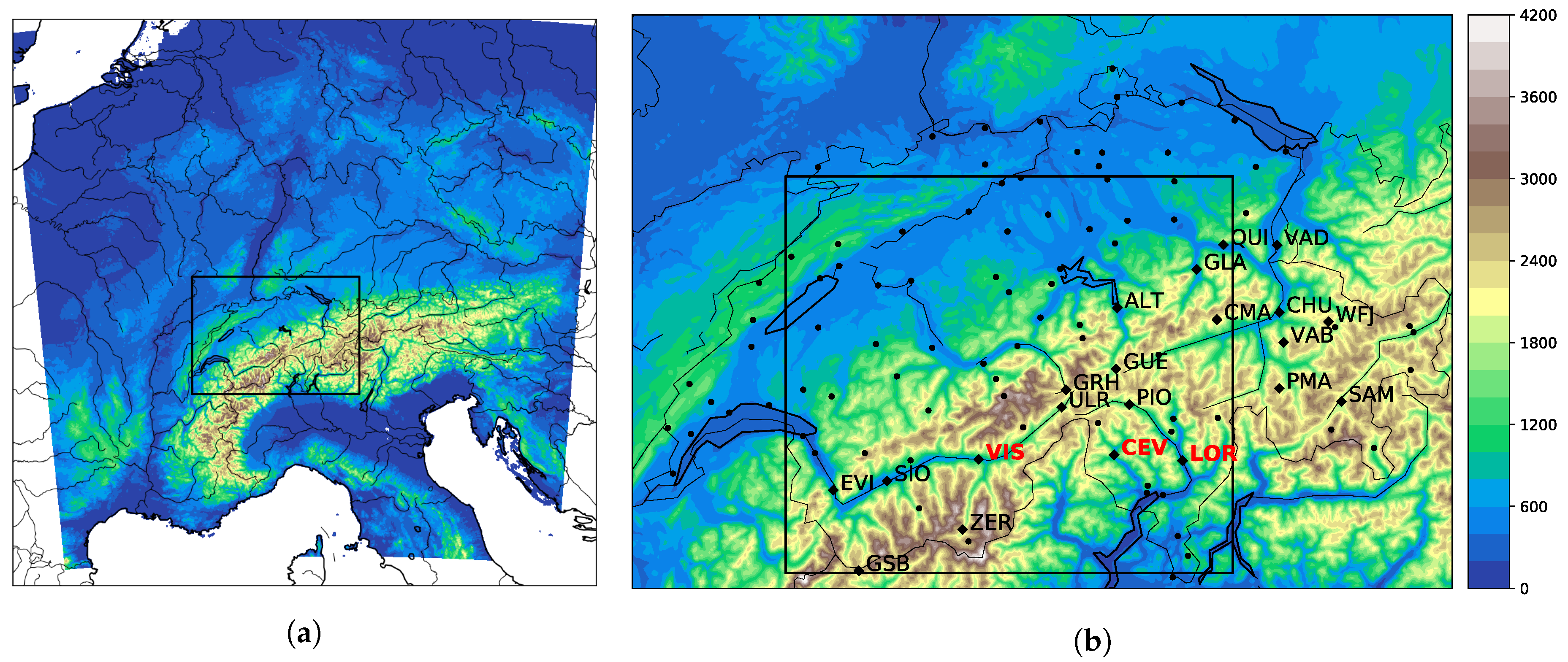
For this study, COSMO version 5.0 is used in a setup close to its current use in numerical weather prediction at MeteoSwiss. The package of physical parameterizations used in this study include a radiative transfer scheme based on the -two-stream approach [29], a single-moment bulk cloud-microphysics parameterization [30], and a turbulent kinetic energy-based surface transfer and PBL parameterization [31,32]. Slope and shadowing effects on radiation are computed following the method of [33,34]. A large model domain has been chosen () to fully cover the European Alps (see Figure 1a); a domain with extensions similar to that in the operational setup at MeteoSwiss. In the vertical direction, a pressure-based hybrid coordinate is used, with 61 stretched model levels ranging from the surface to the model’s top at 20 km. The vertical grid spacing ranges from 20 m for the lowest levels, increases slowly to a grid spacing of about 100 m at 1 km above ground level (AGL), and to about 1100 m at the model top. There are 20 model levels below 1 km. Due to the vertical staggering, the centers of the lowest grid boxes (i.e., mass points) and the horizontal velocities are located at about 10 m AGL. Rayleigh damping is applied in the uppermost levels.
The parameterization of the land surface processes is performed with the multilayer soil model TERRA-ML [35]. The soil parameters (e.g., pore volume, field capacity, heat capacity, and wilting point) are prescribed according to one of eight predefined soil types. Vegetation is specified by means of prescribed seasonally varying leaf area index, fractional plant cover, and root depth. The soil model is run with 10 soil layers with thicknesses ranging from 1 cm to m and a total soil depth of m. This setup was chosen so that the soil temperature and moisture could be initialized from an available climate simulation (see below), thus strongly reducing spin-up effects in the soil. The surface roughness length in COSMO arises from two contributions. One part depends on the type of land cover in the grid box, and the other part is related to the subgrid-scale variance of the topography [36]. In steep Alpine terrain, the second part usually dominates.
2.2. Experiments
A month-long time period with pronounced thermally driven diurnal winds has been selected: the month of July 2006. The major part of the period is characterized by weak synoptic forcing with strong irradiance and a pronounced diurnal cycle of the wind systems and local orographic convection over the Alps on several days. Because of this latter aspect, July 2006 has been the subject of several previous studies (e.g., [24,37,38,39]). Only during the beginning (5–8) and end (27–30) of the month is precipitation related to synoptic disturbances. All simulations are initialized at 0000 UTC 1 July 2006 and terminated at 0000 UTC 1 August 2006 (UTC = Central European summer time − 2 h). By performing month-long simulations without re-initialization spin-up issues in the soil and the atmosphere are minimized, in particular of the local atmosphere in the valleys (which is not resolved in the driving model).
Initial and six-hourly boundary conditions are provided by the operational analysis of the European Centre for Medium-Range Weather Forecasting (ECMWF) at a horizontal resolution of km. To ensure a short spin-up of the deeper soil layers, all simulations are initialized with soil moisture and temperature distributions that were obtained from the long-term reanalysis-driven climate simulation conducted by [40] with COSMO at a 2 km resolution. The land surface data for the climate simulation were based on the low-resolution land surface datasets (see below). Only the period dominated by weak synoptic forcing between 0000 UTC 9 July and 0000 UTC 27 July 2006 will be evaluated in this study. All mean diurnal cycles presented below relate to this period.
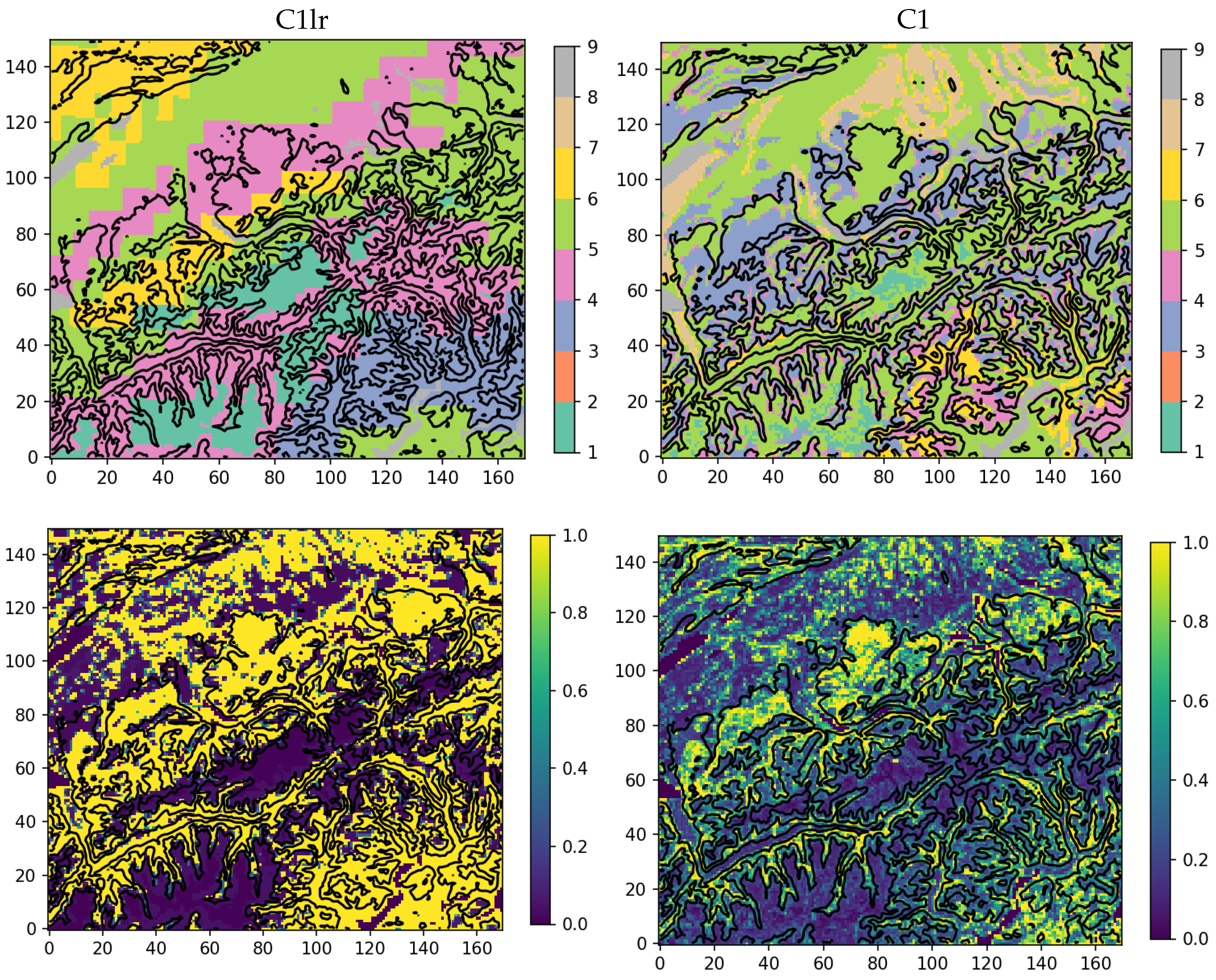
An overview of the main numerical experiments is presented in Table 1. The setups for all simulations are identical, except for differences in the horizontal resolution ( km and km) and in the land surface datasets used to derive the topography, soil, and land cover, see Table 2. The four main simulations (C1, C1lr, C2, and C2lr) allow for a separate assessment of the added value of an increase in horizontal grid spacing and an improved description of the land surface. The high-resolution datasets corresponds to the current operational setup of the high-resolution COSMO run at MeteoSwiss, while the low-resolution datasets correspond to the former operational setup at MeteoSwiss (which is still used at other national weather services). Characteristic differences between the low- and high-resolution datasets are illustrated in Figure 2. Regarding soil type, there are obvious, large differences between the two datasets, while the larger-scale land cover patterns appear to be relatively similar in the two datasets (not shown). Note the large differences with respect to the momentum roughness length. The Rhone valley, for example, is characterized by a large roughness length in C1lr, but a small roughness length in C1, as would be expected for the flat valley floor. Clearly, the high-resolution ASTER terrain data allows for a more realistic representation of the subgrid-scale orography and its impact on the roughness length. To prevent numerical instabilities related to steep terrain, the topography is low-pass-filtered (Raymond filter; [41]) with a cutoff at about in the four main simulations. In order to assess the influence of topography filtering, two additional simulations with a cutoff at about (C1f, C500f) are performed (see Section 3.4).
2.3. Observations
Hourly measurements of 10 m winds, 2 m temperature, 2 m humidity, pressure, and short-wave incoming radiation (ETC) from the MeteoSwiss ANETZ (automatic monitoring network) are used. From the total of 107 stations available for July 2006, only those stations with a pronounced diurnal cycle in the wind speed are selected for further analysis (see Figure 1b). We refer to these as diurnal wind stations. These stations are determined objectively, based on the criterion that the maximum of the mean diurnal cycle of wind speed exceeds 4 m/s. A total of 21 stations fulfill this criterion (see Table 3). Table 3 also includes information on station altitude and site location. With regard to the site location, we distinguish between six different cases: large valleys (lrgval; valley floor width ), medium-sized valleys (medval; ), small valleys (smlval; ), mountain ridges (ridge), mountain passes (pass), and lakeshores (lake).
For each model configuration, the model grid points associated with individual stations are determined by minimizing an optimal distance to the stations. The latter is defined as a weighted average of the horizontal and vertical distances, with stronger weight given to the vertical distance [43].
The hourly wind values correspond to ten-minute means based on vector-averaged instantaneous measurements taken every second. The ten-minute means are calculated for the time interval HH:30.1 to HH:40.0, where HH refers to the corresponding hour.
3. Results
First, an overview of the analysis period is given including some typical results of the valley winds simulated by C1 and C2lr, illustrating the added value of going to a 1 km resolution. Second, the diurnal evolution and frequency distribution of the valley winds are evaluated in detail. Third, additional sensitivity experiments are conducted in order to assess the relative importance of increased model resolution versus better-resolved land surface datasets and to assess the impact of topography smoothing and a further increase of model resolution.
3.1. Overview of July 2006
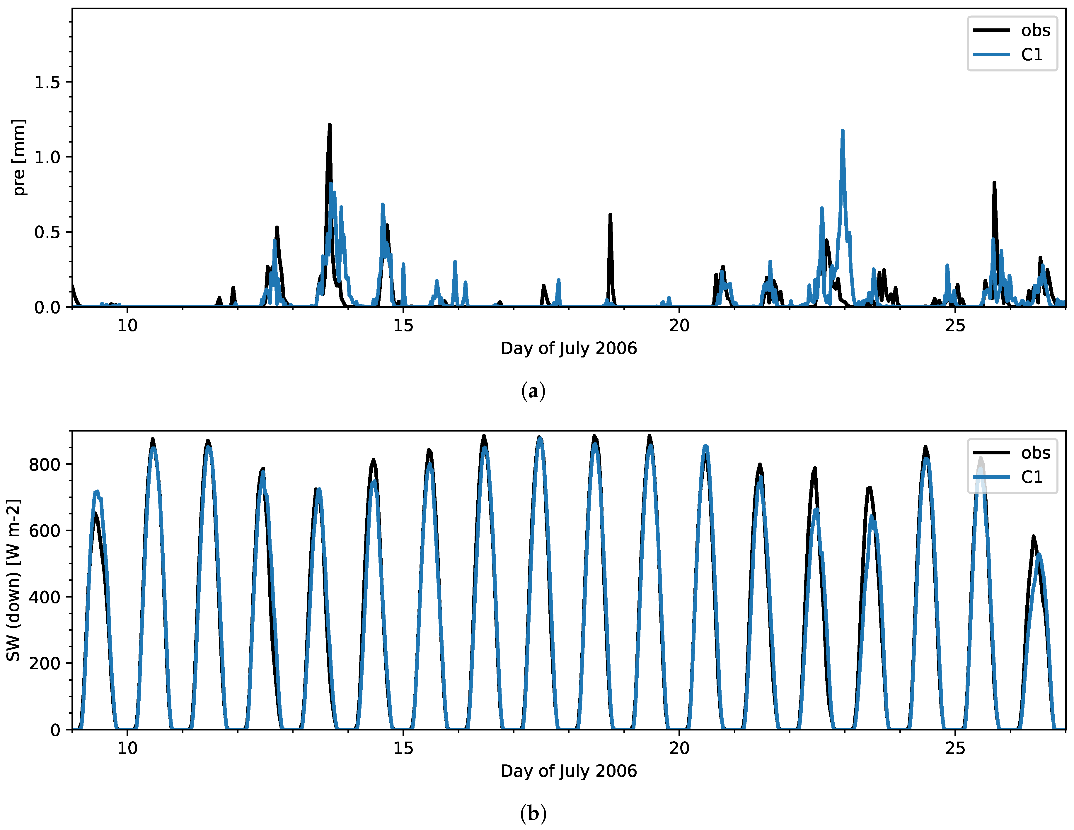
The observed weather in Switzerland during the analysis period in July 2006 is summarized in Figure 3 in terms of mean precipitation and incoming shortwave radiation. On most days, there is some precipitation linked to local deep convection, but the area affected by cloud cover is relatively small as the irradiance remains high. Only in the beginning (5–8) and end (27–30) of the month is there some precipitation related to synoptic disturbances (not shown). The impact of the fair weather and the precipitation episodes is imprinted on the evolution of the soil moisture and the surface sensible heat fluxes (not shown).
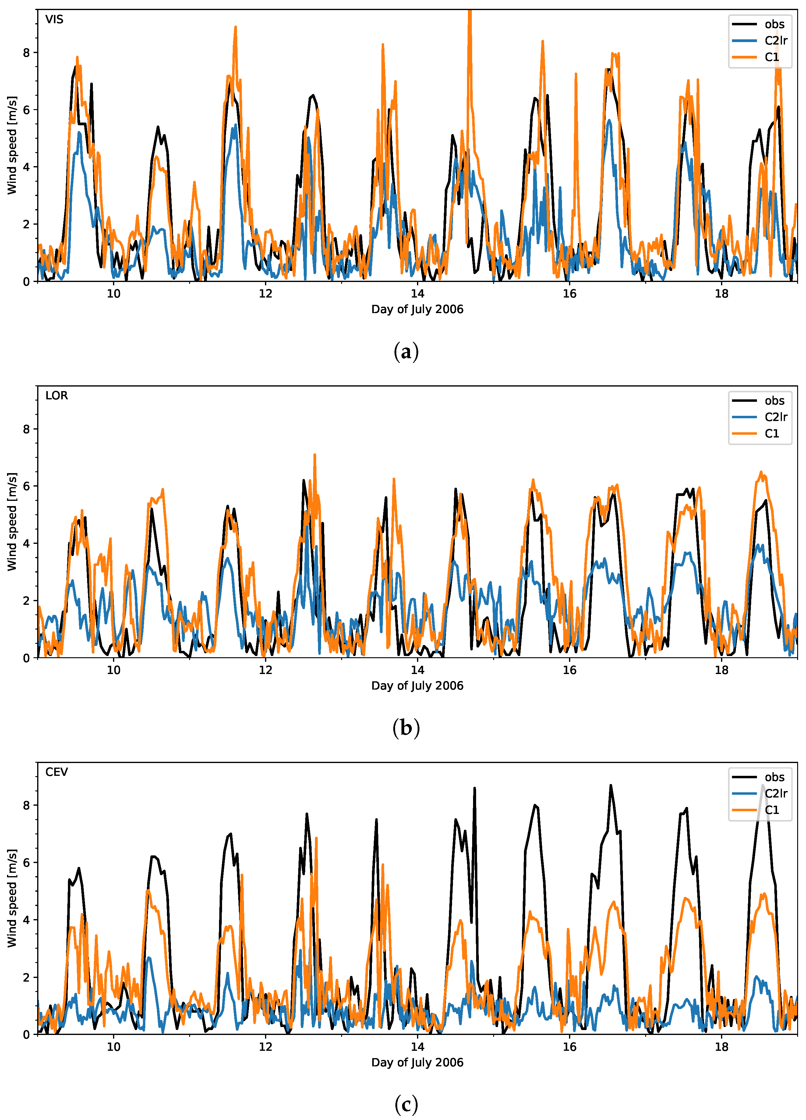
Exemplary results of the 10 m wind speed as simulated by C2lr and C1 (corresponding approximately to the old and new operational model setup at MeteoSwiss) in comparison to observations is shown in Figure 4 for three stations: one in a large valley, one in a medium-sized valley, and one in a small valley, as defined in Table 3. The observations show a pronounced diurnal cycle of the wind speed in all three valleys, with weak winds during the night and strong winds during the day. Maximum daytime velocities are typically 5 m/s to 8 m/s. Turning to the simulated winds, the diurnal cycle is generally well captured by C1 for the two larger valleys, but the simulated amplitude is too weak in the small valley. In contrast, the winds simulated by C2lr are generally too weak, in particular for the smaller two valleys. These are fairly typical findings, as will be shown in the following section.
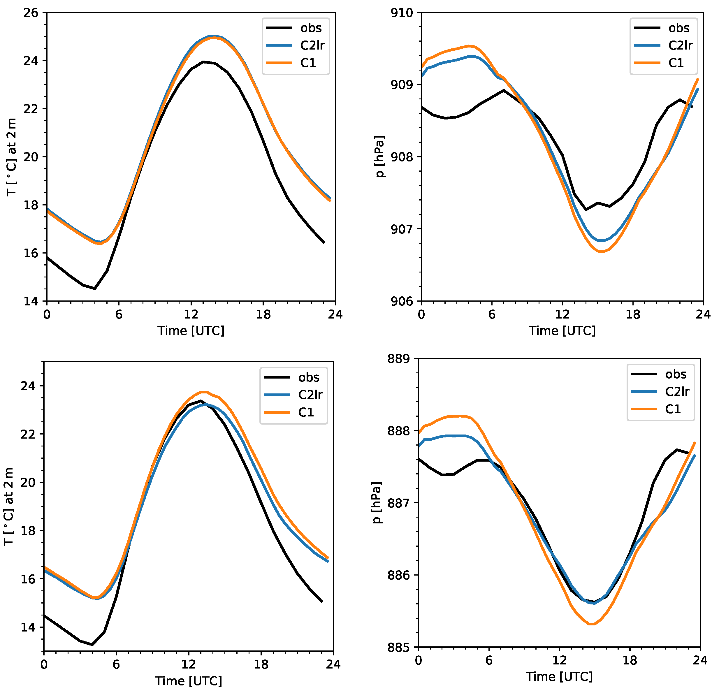
This section is concluded by a basic evaluation of simulated 2 m temperature and surface pressure (Figure 5), two important quantities related to the forcing of the diurnal winds. The figure shows the mean diurnal cycles of the two quantities averaged over all Swiss stations and over the diurnal wind stations (see Figure 1b). Averaged over all stations, both simulations (C2lr, C1) exhibit an overall warm bias and slightly underestimate the diurnal temperature amplitude, due to a stronger nighttime warm bias. A nighttime warm bias is a common feature of the COSMO model, likely due to deficiencies in the parameterization of turbulence and land-atmosphere exchange [44]. Averaged over the diurnal wind stations, the daytime warm bias is substantially reduced, but the underestimation of the diurnal amplitude is increased. Despite these temperature biases, the diurnal pressure amplitude is overestimated for both regions, in particular for the average over all stations. This overestimation suggests an overly large energy input into the boundary layer, possibly resulting in an overly deep and/or overly warm boundary layer, in particular over the non-mountainous regions. Consistent with the bias in the diurnal pressure amplitude, the simulated daytime boundary layer during the analysis period is found to be both too warm and too deep over the Swiss Plateau, as found by comparison with radiosonde data from Payerne (not shown). For the mountain regions, no information is available on the vertical temperature structure of the atmosphere. For the comparison of the 2 m temperature with observations, a simple bias correction due to height differences has been applied to the model data (). While the impact of the correction on the average over all stations is minimal, for the average over the diurnal wind stations it results in an temperature increase of about K for C2lr and K for C1. The corresponding bias correction for pressure uses a gradient of .
3.2. Evaluation of the Diurnal Valley Winds
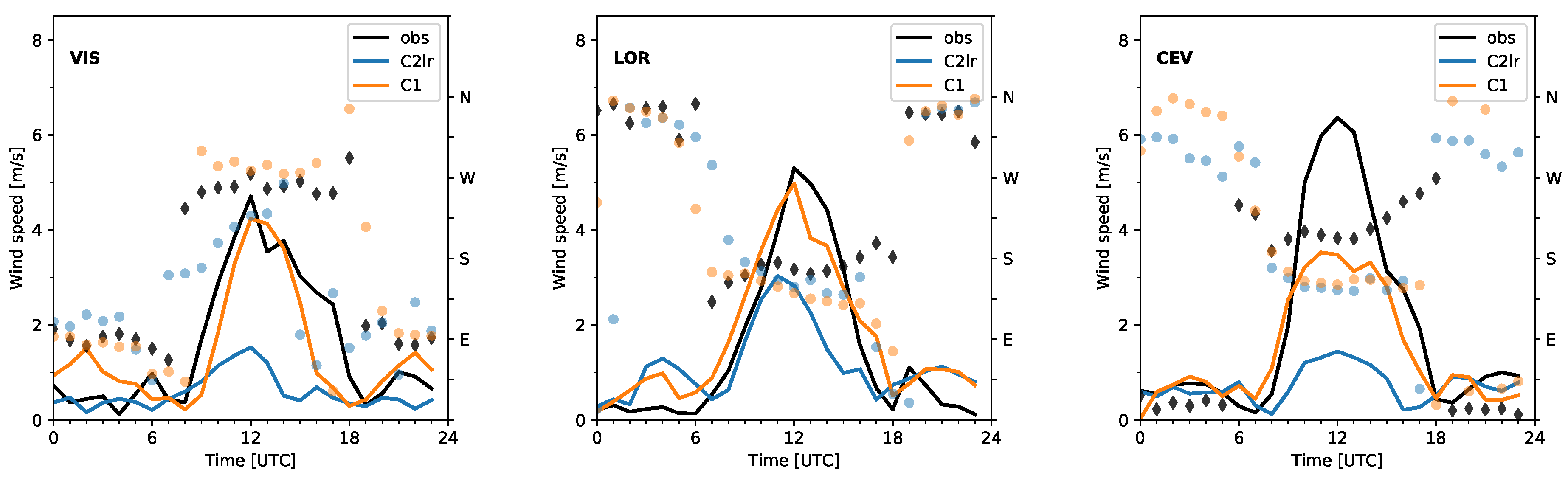
The 10 m wind, as simulated by the two simulations C2lr and C1, is compared with observations in terms of the mean diurnal cycle in Figure 6 for the three stations previously introduced. The differences between the two simulations and the observations can now be more clearly seen, compared to the time series discussed in the previous paragraph. For the station in the large valley, VIS, the diurnal cycle is well represented by C1, both in terms of wind speed and wind direction, but it is virtually non-existent for C2lr. Note that the period of strong up-valley winds is somewhat too short in C1. Similar results hold for the station LOR, with somewhat improved skill for C2lr. For the station in the small valley, CEV, the maximum amplitude is still underestimated even by C1, and there is a bias in the up-valley wind direction. The corresponding results for all diurnal wind stations are shown in Figure A1 in the Appendix. The analysis for all stations confirms the above results: generally closer agreement with the observations for C1 compared with C2lr, generally good skill for the stations in large valleys, and an underestimation of the strength of the valley winds for stations located in small valleys. Going into more detail, the simulated frequency distribution of the wind direction and the wind speed for the three stations is compared with observations in Figure 7 for the up-valley wind period (1000–1800 UTC). Figure 7 confirms the improved skill for C1 in comparison to C2lr, in particular for the wind speed and the overall wind regime for VIS. For the two stations in the larger valleys (VIS and LOR), both the observed and C1 winds are relatively strong and up-valley most of the time, while they are weaker for C2lr and more variable for VIS.
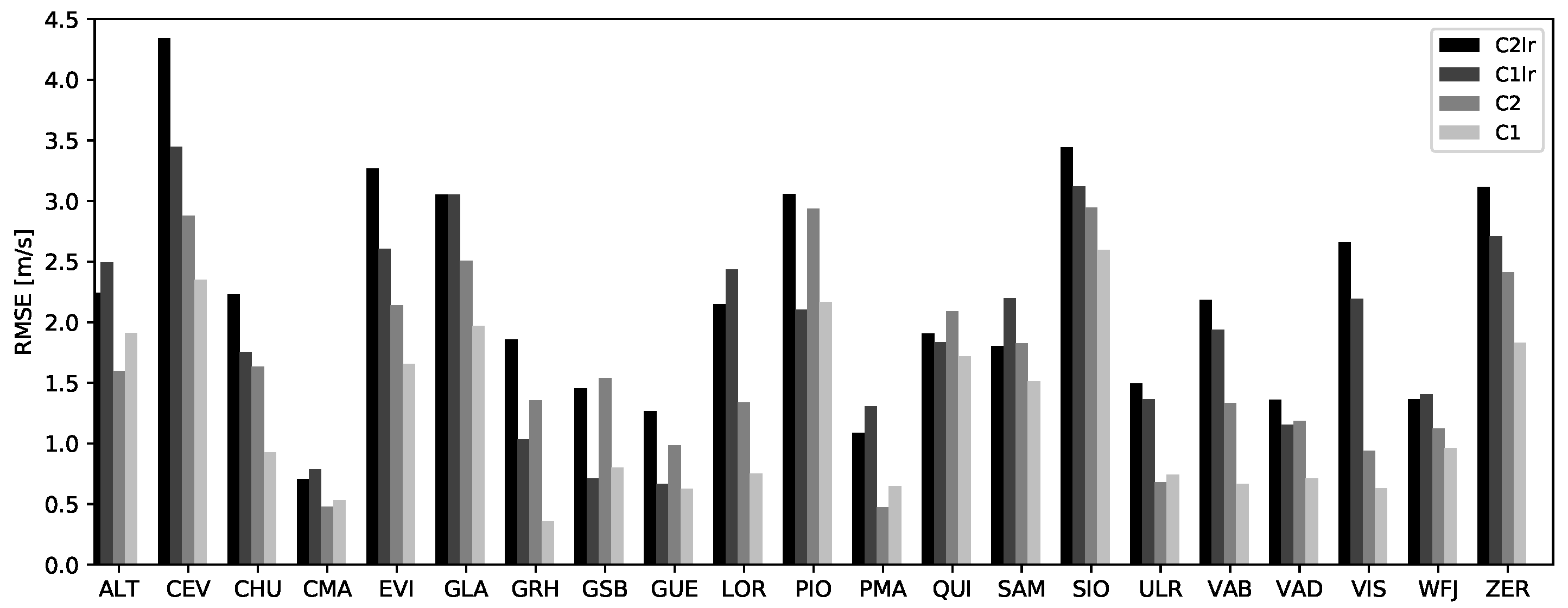
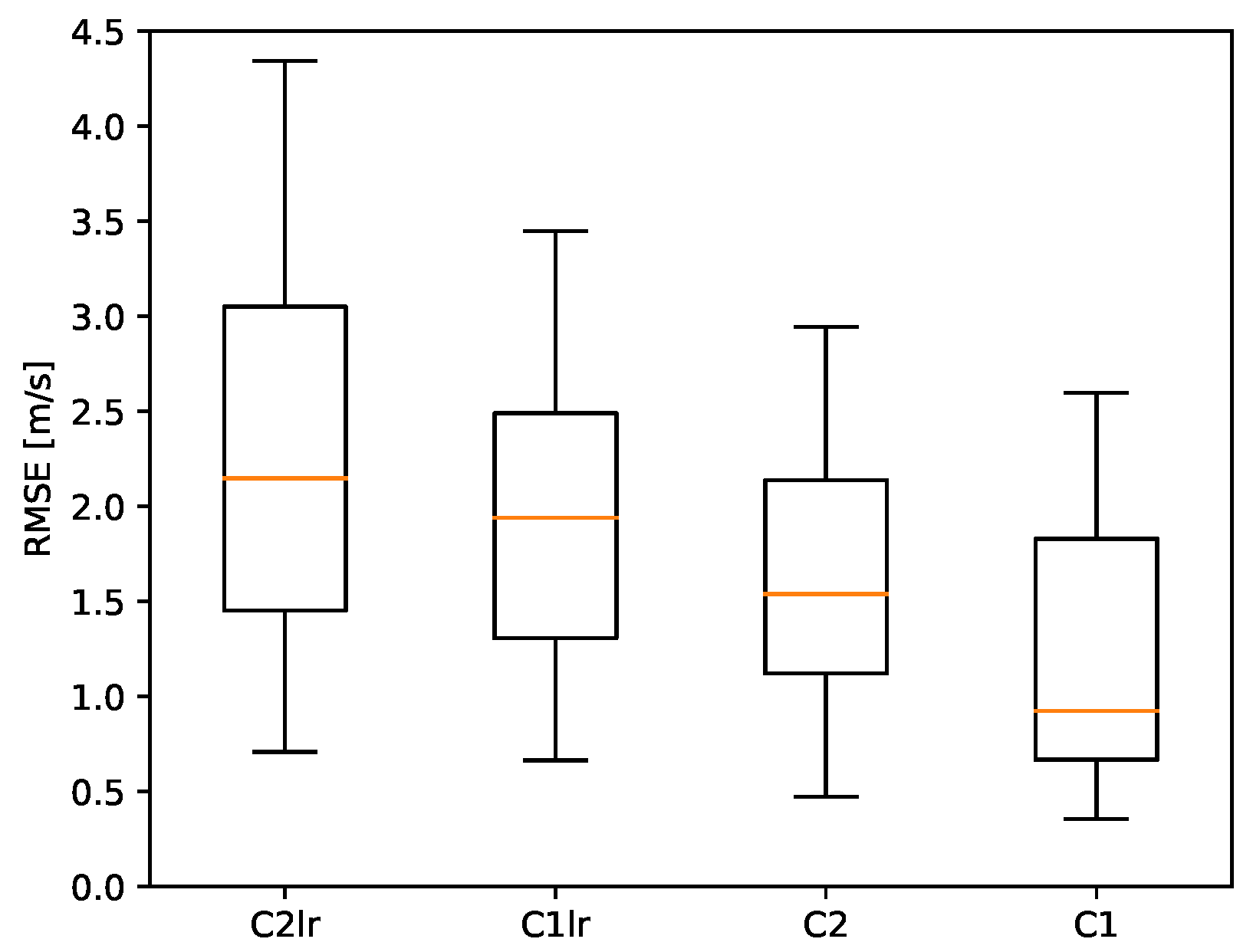
Next, the evaluation is extended to the four main simulations C2, C1, C2lr, and C1lr. As the largest differences between observations and simulations are found during the daytime up-valley wind, we focus on the daytime maximum winds. Furthermore, the daytime near-surface winds are more strongly correlated with the strength of the bulk valley wind than the nighttime near-surface winds and hence are a better measure of the strength of the bulk valley wind. The root-mean-square error (RMSE) of the mean diurnal cycle in the period 10–14 UTC is shown in Figure 8. It can be considered a robust measure of the difference in the mean maximum valley wind. As the typical model error consists of an underestimation of the maximum wind, the RMSE corresponds roughly to the bias of the mean maximum valley wind (with opposite sign). For all stations, the error for C1 is smaller than that for C2lr. Thus, C1 is systematically closer to observations than C2lr. The picture becomes clearer in terms of the overall statistics shown in Figure 9. Surprisingly, the error of the low-resolution simulation with high-resolution land surface data (C2) is on average smaller than the error for the high-resolution simulation with low-resolution land surface data (C1lr). Overall, there is a clear trend of reduced error from C2lr to C1lr, from C1lr to C2, and from C2 to C1. The median RMSE is around 2 m/s for C2lr and C1lr, about m/s for C2, and below 1 m/s for C1.
Figure 9 shows clearly that only increasing the grid resolution—and keeping the older low-resolution land-surface data—does not lead to much improvement in the average skill, but combining increased grid resolution with higher-resolution land surface data leads to a significant reduction of the error (C1).
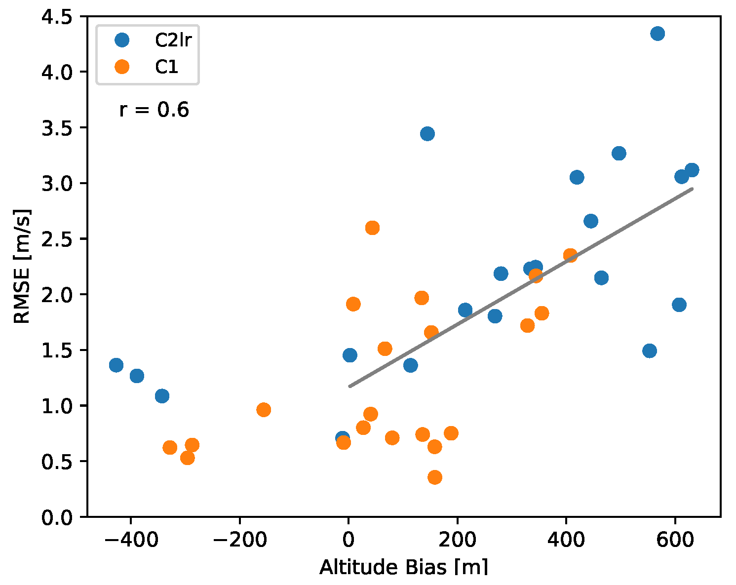
Everything else kept equal, there is a significant increase in average skill with an increased model grid resolution (C2 vs. C1). As the different valleys vary strongly in their characteristic dimensions, differences in the skill for individual stations can be expected (as seen in Figure 8). What fraction of the station-to-station variability can be explained by differences in the fidelity of the model topography for a particular valley and location? As a simple measure of the fidelity of the model topography, we consider the bias of the grid point altitude with respect to the station altitude. Figure 10 shows the resulting scatter plot of RMSE versus altitude bias. Errors in grid point altitude, positive biases corresponding to an underestimation of the valley depth in the simulations, are clearly related to the RMSE. The anomaly correlation is 0.6. With few exceptions, small altitude biases result in a smaller RMSE.
In summary, accurate simulation of the valley winds requires sufficient grid resolution to resolve the valley topography, but also good-quality high-resolution land surface datasets (cf. Figure 9).
3.3. Impact of Land Surface Datasets
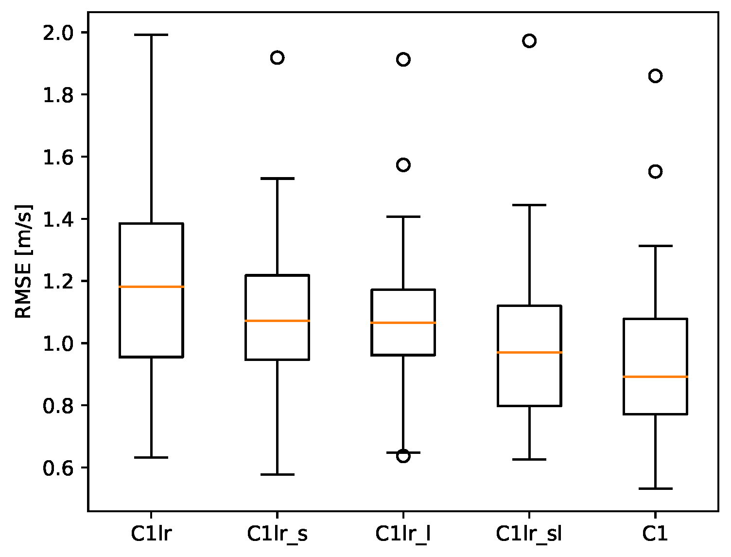
It has been shown that the use of high-resolution land surface datasets is essential for obtaining an improved model performance at km grid spacing. Which of the land surface datasets, topography, soil type, land cover, is primarily responsible for the improvements? To address this question, several additional model runs were carried out. The resulting RMSEs of the simulated mean diurnal cycle is summarized in Figure 11. It is found that all three datasets contribute to an improvement in terms of the average statistics over all stations. In terms of the median RMSE, all three datasets contribute about equally to the reduction of the error. In summary, high-resolution topography, soil type, and land cover datasets are required for optimal results. As illustrated in Figure 2, high-resolution topography is needed not only for a more accurate representation of the resolved topography but also of the subgrid-scale topography used, for example, in the derivation of the momentum roughness length.
3.4. Impact of Topography Smoothing and Grid Resolution
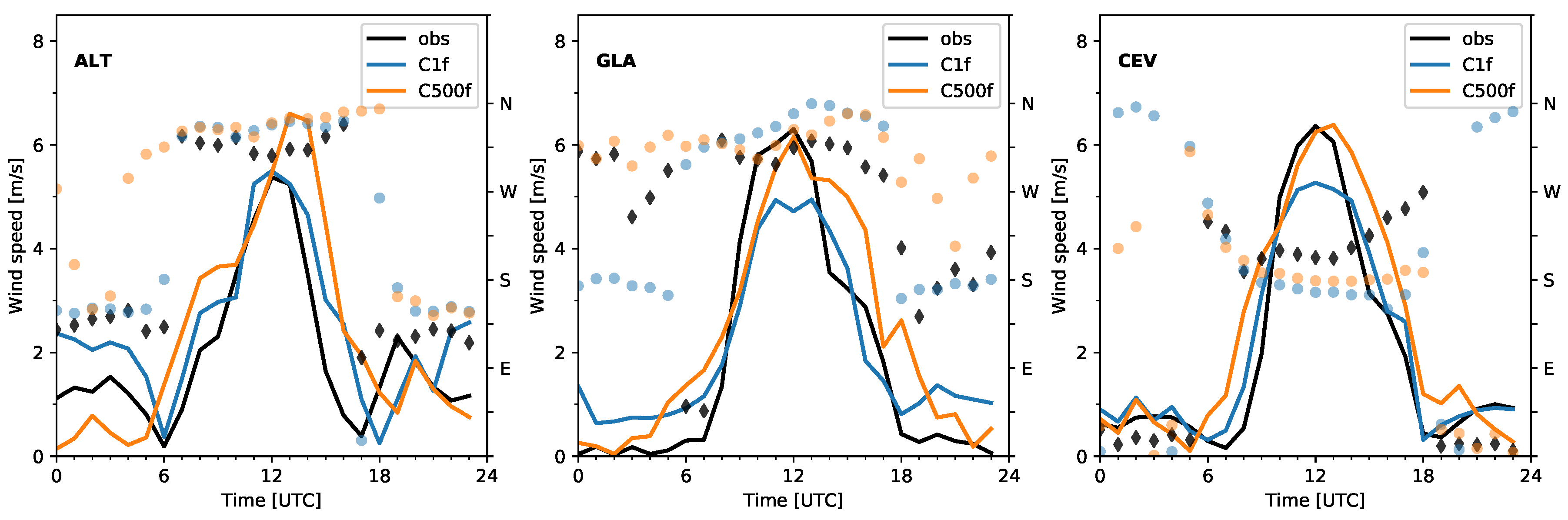
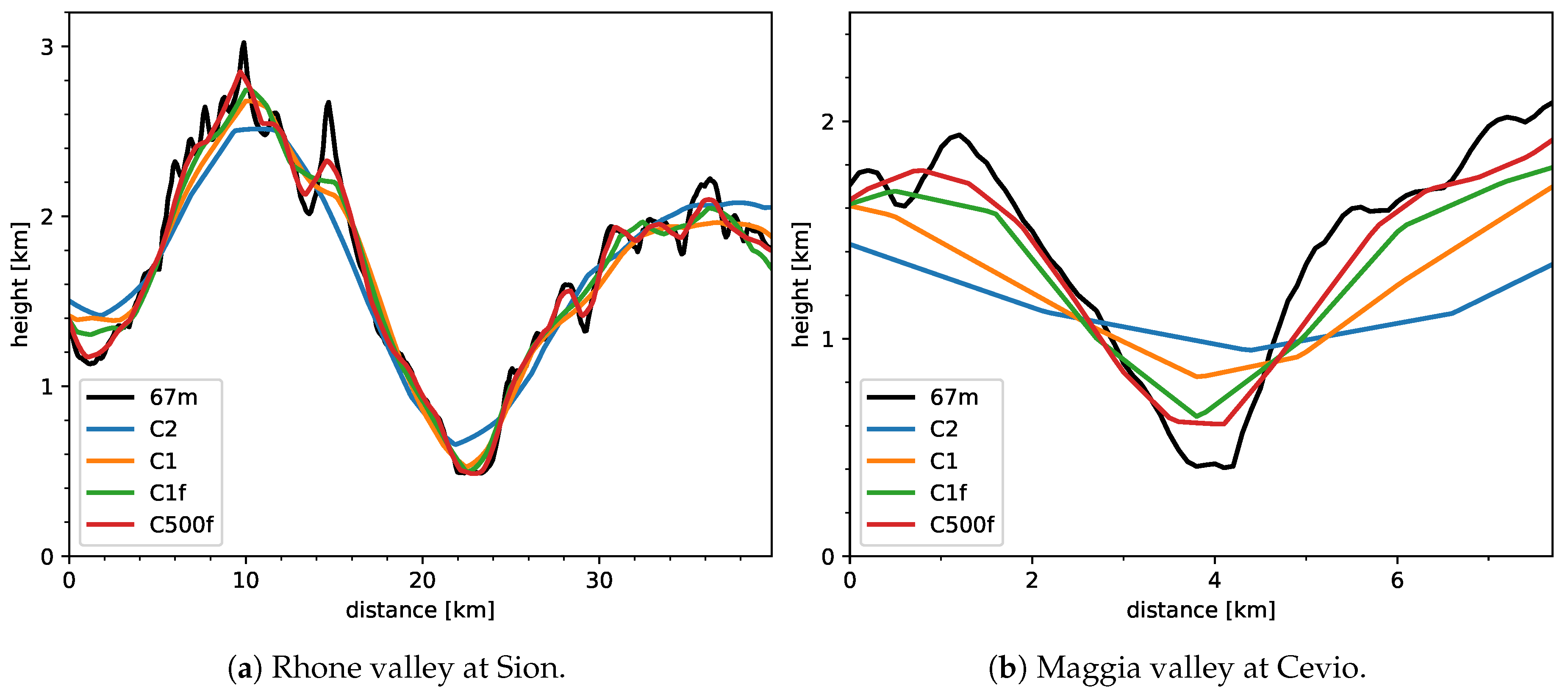
The accuracy of the model topography depends not only the topography dataset used and the model grid spacing, but also on the amount of smoothing applied to the model topography. It is common practice to smooth the topography in order to remove topographic forcings originating from the smallest scales, which can not be accurately represented by the model numerics and would just result in numerical noise. Topography smoothing may also help with numerical stability by reducing the maximum inclination of the slopes. In the COSMO model, a Raymond filter [41] is used to smooth the model topography. The operational setup uses relatively strong smoothing, with a cutoff at approximately 5 (filter parameter ), in order to ensure numerical stability. Results for Simulation C1f, a km model run with reduced smoothing (cutoff at approximately 3.5; ), and for Simulation C500f, a 550 m run with reduced smoothing, are shown in Figure 12. In all three setups, the filter is applied twice. To ensure a stable model run, the implicitness of vertical fast mode integration had to be increased. As expected, the reduced filtering (and the higher resolution) results in significantly steeper slopes but also reduced altitude biases (see Table 4) and a more accurate representation of the valley topography in terms of the valley cross section (Figure 13). The more accurate representation of the topography leads to an improved simulation of the valley winds (compare Simulation C1f in Figure 12 to Simulation C1 in Figure A1. Thus, for an accurate simulation of the valley winds, it is recommended that the strength of the topography smoothing be reduced.
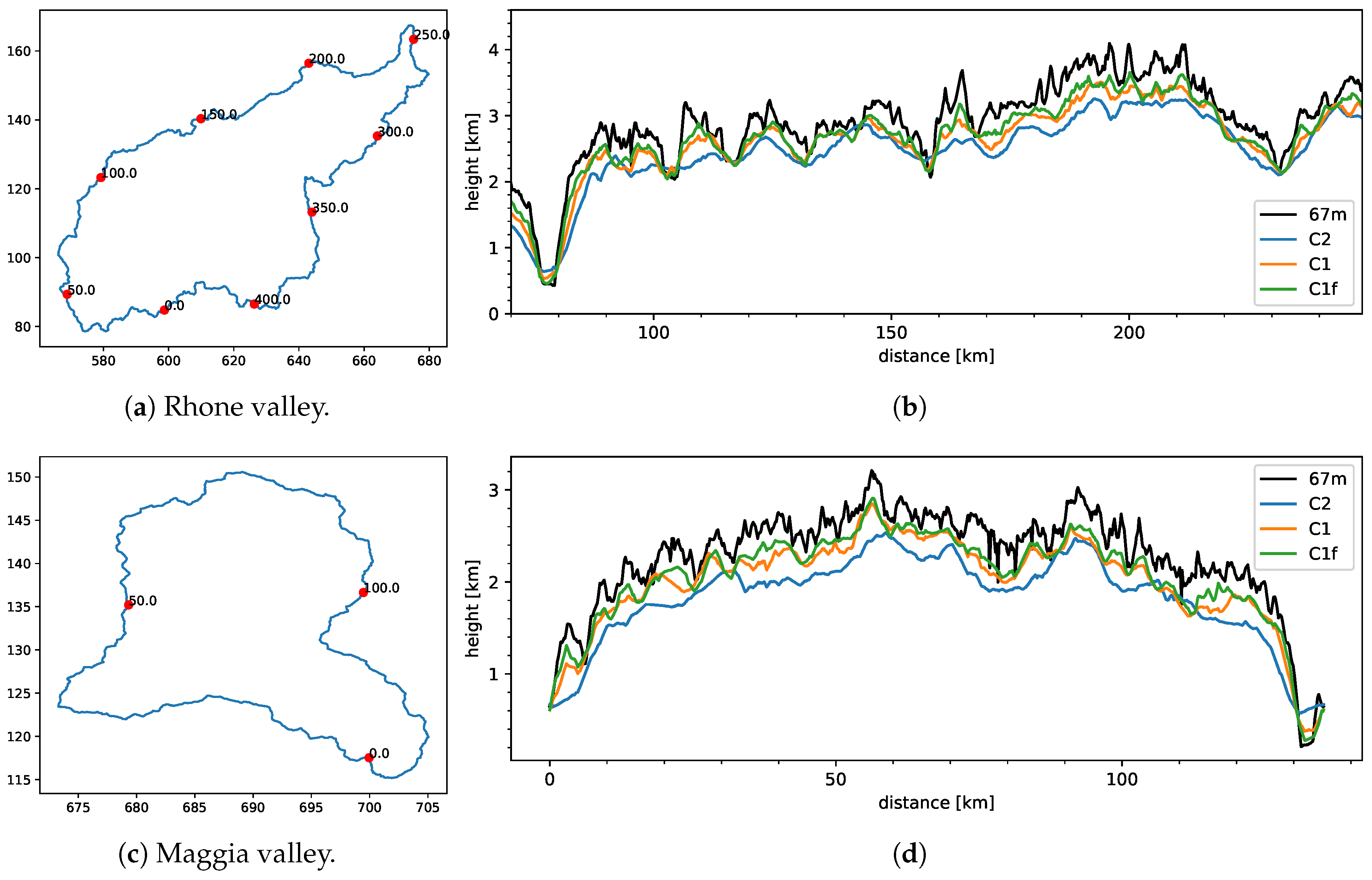
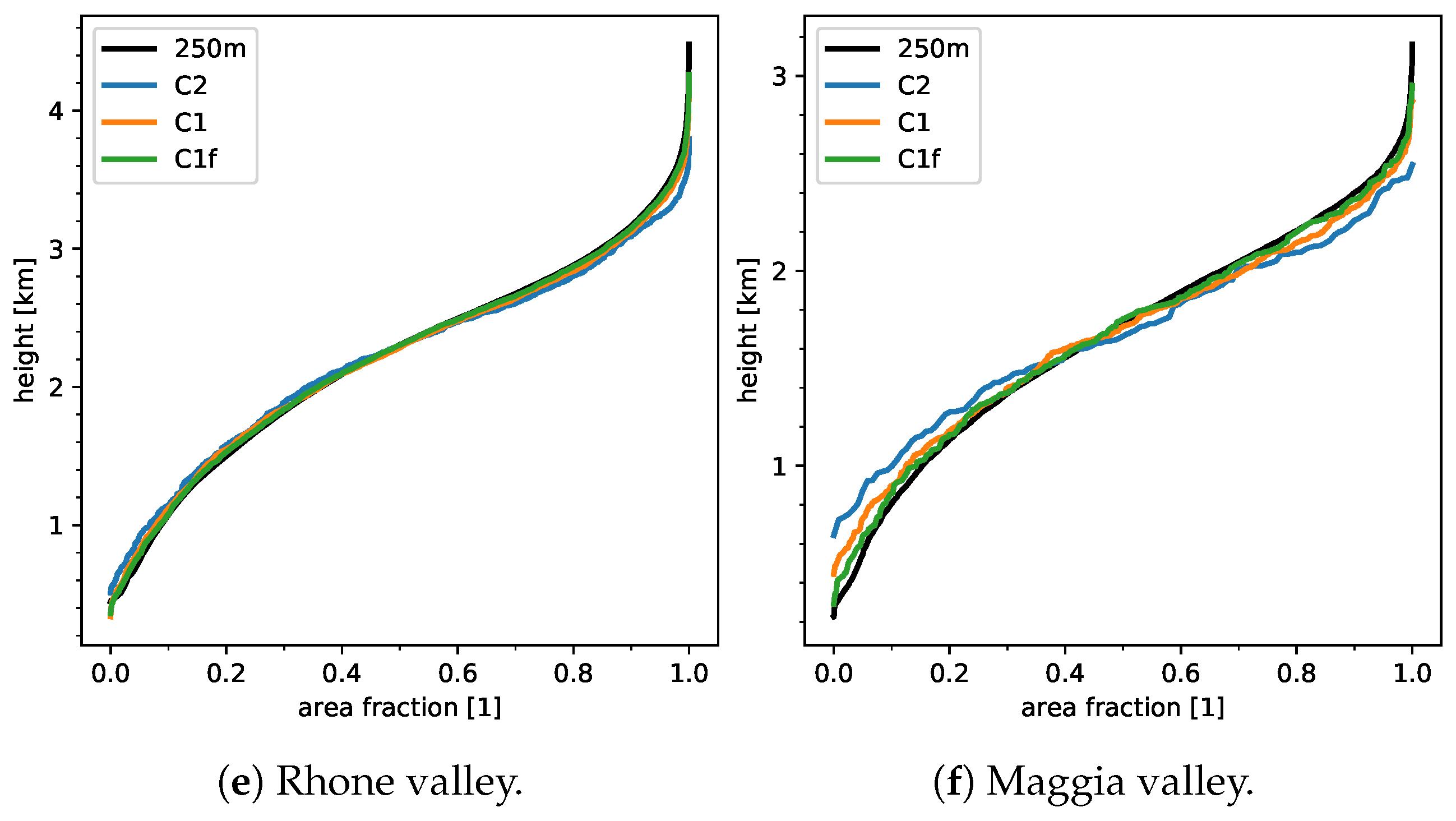
Increasing the resolution further to a 500 m grid spacing, leads to mixed results, as seen for Simulation C500f in Figure 12 (in comparison to C1f). On the one hand, the winds in the narrow valleys are further improved (e.g., GLA and CEV); on the other hand, there is an overestimation of the maximum wind speed in the large valley (e.g., ALT). Other factors, such as an accurate representation of the land-atmosphere interface, likely become more important once the grid resolution is no longer the main limiting factor. Based on valley wind theory and the concept of the topographic amplification factor [9,17], two important factors are the accurate representation of the local valley topography and of the area–height distribution in the valley catchment, as the along-valley wind is driven by local (along-valley) and regional (valley-plain) pressure differences. Furthermore, the height of the ridgeline enclosing the valley catchment may play an important role with regard to the interaction of the valley flow with larger-scale flows. The impact of filtering and model resolution on these quantities is illustrated in Figure 14. With respect to the area–height distribution, the Rhone valley is well represented at km (C1 and C1f), while the smaller Maggia valley is still underresolved, although the bias is significantly smaller for C1f. The height of the ridgeline is much improved with higher resolution and reduced filtering.
4. Conclusions
The near-surface representation of thermally driven winds in the Swiss Alps in long-term simulations at 2.2 and 1.1 km resolutions has been systematically evaluated against surface observations for an 18-day summer period with weak synoptic forcing and intense solar heating. The importance of grid resolution, the choice of land surface datasets, and the topography filtering for the accurate simulation of the thermally induced winds is assessed. In comparison to previous work, this study includes all moderate to strong diurnal wind stations in the Swiss Alps and thus is representative of large and small valleys.
The evaluation of the simulations showed the following results:
- At km grid spacing, the diurnal cycle of the valley winds is poorly simulated for most stations, in particular for the simulations using the lower-resolution land surface datasets. At a km resolution, the diurnal cycle is well represented in most large (e.g., Rhein valley at Chur and Rhone valley at Visp) and medium-sized valleys (e.g., Linth valley at Glarus). In the smaller valleys (e.g., Maggia valley at Cevio), the amplitude of the valley wind is still significantly underestimated, even at a 1.1 km resolution. The median RMSE of the mean daytime maximum wind speed is reduced from around 2 m/s for the two simulations with lower-resolution land surface data (C2lr, C1lr) to less than 1 m/s for the km simulation with higher-resolution land surface data (C1).
- The sensitivity experiments show that the use of high-resolution land surface datasets, for topography, the soil characteristics as well as the land cover is essential to achieve an improved representation of the valley winds. Thus, in contrast to [24], we find a significant improvement of the simulated winds at a km resolution, in comparison to a km resolution. This can be attributed to the fact that, in [24], the authors did not use the higher-resolution land surface datasets, as these were not yet available for the COSMO model, and that they considered only a small subset of the stations (located in the larger valleys).
- Not surprisingly, the fidelity of the model valley topography is a key factor for a good representation of the valley wind. It was found that a simple measure of this fidelity—the grid point altitude bias—is a reasonable predictor for the accuracy of the simulated winds. Furthermore, it was shown that a reduced filtering of the topography (cutoff at 3.5), in comparison to the operational setup at MeteoSwiss (cutoff at 5), results in a further improvement of the simulated winds, in particular for the smaller valleys. The resolution requirement for a good representation of the along-valley wind seems to be surprisingly moderate. Resolving the valley floor cross section with only 1–2 grid points yields good results in most cases.
Our findings demonstrate that, as NWP models reach 1 km grid spacing, a good representation of the main diurnal wind systems, in particular the daytime along-valley winds, can be obtained in an operational NWP model, provided that high-resolution land surface data is used. Even if these winds are only one component of the complex-terrain boundary layer, they can serve as a useful benchmark for high-resolution numerical weather prediction models over complex terrain. In contrast to other complex-terrain phenomena, the strength of the near-surface along-valley winds can be evaluated with routine wind observations. The accurate simulation of the near-surface component of the thermally driven diurnal wind systems is just a first step in a skilful forecast for mountain regions. Long-term observations of the vertical and horizontal structure of the diurnal wind systems and the mountain atmosphere over long periods (e.g., [45]) are required for more detailed evaluation of NWP models, improved physical parameterizations adapted to complex terrain, and hence better forecasts of mountain weather.
Author Contributions
J.S. wrote the paper and prepared the figures. S.B. and O.F provided input and discussion for carrying out the experiments and commented on the paper.
Funding
Funding for Steven Böing and Juerg Schmidli was provided by MeteoSwiss through C2SM. Juerg Schmidli was also partly supported by the Hans Ertel Centre for Weather Research. This German research network of Universities, Research Institutes and the Deutscher Wetterdienst is funded by the BMVI (Federal Ministry of Transport and digital Infrastructure).
Acknowledgments
We would like to thank Jean-Marie Bettems, Daniel Lüthi, and Guy de Morsier for technical support, and the members of the COSMO-NExT team at MeteoSwiss for feedback on model setup and simulation results. Simulations were performed on the CRAY XE6 at the Swiss National Supercomputing Centre (CSCS) using COSMO. Analyses and figures were produced using Python and open source software Matplotlib [46].
Conflicts of Interest
The authors declare no conflict of interest.
Appendix A
Figure A1.
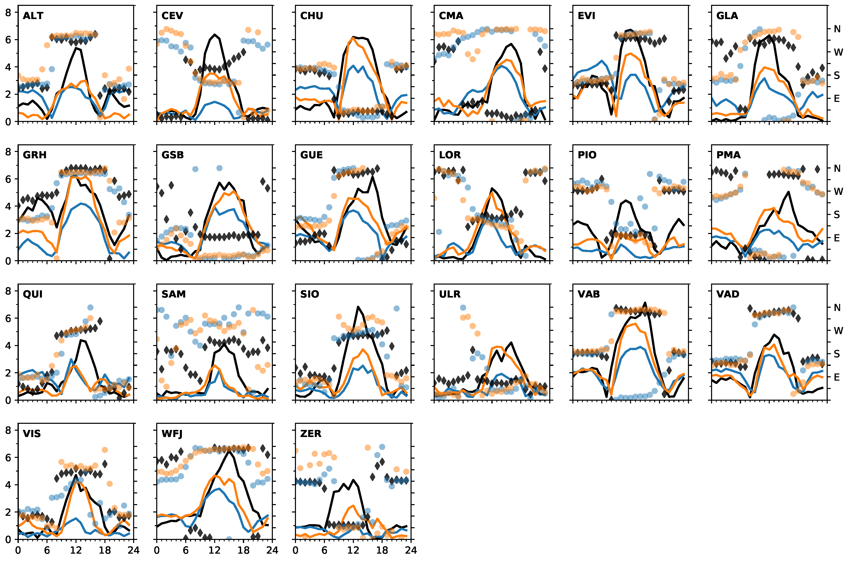
Mean diurnal cycle of wind speed (lines) and wind direction (symbols), as in Figure 6, but for all diurnal wind stations for C2lr (blue) and C1 (red).
Figure A1.
Mean diurnal cycle of wind speed (lines) and wind direction (symbols), as in Figure 6, but for all diurnal wind stations for C2lr (blue) and C1 (red).

References
- Schmutz, C.; Schmuki, D.; Duding, O.; Rohling, S. Aeronautical Climatological Information Sion LSGS; Arbeitsbericht 209; Federal Office of Meteorology and Climatology (MeteoSwiss): Zurich, Switzerland, 2004; Available online: http://www.meteoschweiz.admin.ch (accessed on 22 February 2018).
- Banta, R.M. The role of mountain flows in making clouds. In Atmospheric Processes over Complex Terrain; Number 23 in Meteorological Monographs; American Meteorological Society: Boston, MA, USA, 1990; pp. 229–283. [Google Scholar]
- Zardi, D.; Whiteman, C.D. Observations of thermally developed wind systems in mountainous terrain. In Mountain Weather Research and Forecasting—Recent Progress and Current Challenges; Springer: Berlin, Germany, 2013; pp. 35–122. [Google Scholar]
- Rotach, M.W.; Calanca, P.; Graziani, G.; Gurtz, J.; Steyn, D.G.; Vogt, R.; Andretta, M.; Christen, A.; Cieslik, S.; Connolly, R.; et al. Turbulence structure and exchange processes in an alpine valley: The Riviera project. Bull. Am. Meteorol. Soc. 2004, 85, 1367–1385. [Google Scholar] [CrossRef]
- Schmidli, J. Daytime heat transfer processes over mountainous terrain. J. Atmos. Sci. 2013, 70, 4041–4066. [Google Scholar] [CrossRef]
- Rotach, M.W.; Gohm, A.; Lang, M.; Leukauf, D.; Stiperski, I.; Wagner, J.S. The world is not flat: Implications for the global carbon balance. Front. Earth Sci. 2015, 76. [Google Scholar] [CrossRef]
- Serafin, S.; Adler, B.; Cuxart, J.; De Wekker, S.F.J.; Gohm, A.; Grisogono, B.; Kalthoff, N.; Kirshbaum, D.J.; Rotach, M.W.; Schmidli, J.; et al. Exchange processes in the atmospheric boundary layer over mountainous terrain. Atmosphere 2018, 9, 102. [Google Scholar] [CrossRef]
- Wagner, A. Theorie und Beobachtung der periodischen Gebirgswinde. Gerl. Beitr. Geophys. 1938, 52, 408–449. [Google Scholar]
- Steinacker, R. Area-height distribution of a valley and its relation to the valley wind. Contrib. Atmos. Phys. 1984, 57, 64–71. [Google Scholar]
- Egger, J. Thermally forced flows: Theory. In Atmospheric Processes over Complex Terrain; Number 23 in Meteorological Monographs; American Meteorological Society: Boston, MA, USA, 1990; pp. 43–58. [Google Scholar]
- Neininger, B.; Liechti, O. Local winds in the upper Rhone valley. GeoJournal 1984, 8, 265–270. [Google Scholar] [CrossRef]
- Hennemuth, B.; Schmidt, H. Wind phenomena in the Dischma valley during DISKUS. Arch. Meteorol. Geophys. Bioklimatol. 1985, 35, 361–387. [Google Scholar] [CrossRef]
- Whiteman, C.D. Observations of thermally developed wind systems in mountainous terrain. In Atmospheric Processes over Complex Terrain; Number 23 in Meteorological Monographs; American Meteor Society: Geneseo, NY, USA, 1990; pp. 5–42. [Google Scholar]
- Henne, S.; Furger, M.; Nyeki, S.; Steinbacher, M.; Neininger, B.; de Wekker, S.F.J.; Dommen, J.; Spchtinger, N.; Stohl, A.; Prévôt, A.S.H. Quantification of topographic venting of boundary layer air to the free troposphere. Atmos. Chem. Phys. 2004, 4, 497–509. [Google Scholar] [CrossRef]
- Rotach, M.W.; Zardi, D. On the boundary-layer structure over highly complex terrain: Key findings from MAP. Q. J. R. Meteorol. Soc. 2007, 133, 937–948. [Google Scholar] [CrossRef]
- Rampanelli, G.; Zardi, D.; Rotunno, R. Mechanisms of up-valley winds. J. Atmos. Sci. 2004, 61, 3097–3111. [Google Scholar] [CrossRef]
- Schmidli, J.; Rotunno, R. Mechanisms of along-valley winds and heat exchange over mountainous terrain. J. Atmos. Sci. 2010, 67, 3033–3047. [Google Scholar] [CrossRef]
- Schmidli, J.; Rotunno, R. Influence of the valley surroundings on valley-wind dynamics. J. Atmos. Sci. 2012, 69, 561–577. [Google Scholar] [CrossRef]
- Wagner, J.S.; Gohm, A.; Rotach, M.W. The impact of valley geometry on daytime thermally driven flows and vertical transport processes. Q. J. R. Meteorol. Soc. 2015, 141, 1780–1794. [Google Scholar] [CrossRef]
- Zängl, G. Numerical errors above steep topography: A model intercomparison. Meteorol. Z. 2004, 13, 69–76. [Google Scholar] [CrossRef]
- Chow, F.K.; Weigel, A.P.; Street, R.L.; Rotach, M.W.; Xue, M. High-resolution large-eddy simulations of flow in a steep Alpine valley. Part I: Methodology, verification, and sensitivity experiments. J. Appl. Meteorol. Climatol. 2006, 45, 63–86. [Google Scholar] [CrossRef]
- Weigel, A.P.; Chow, F.K.; Rotach, M.W.; Street, R.L.; Xue, M. High-resolution large-eddy simulations of flow in a steep Alpine valley. Part II: Flow structure and heat budgets. J. Appl. Meteorol. Climatol. 2006, 45, 87–107. [Google Scholar] [CrossRef]
- Schmidli, J.; Poulos, G.S.; Daniels, M.H.; Chow, F.K. External influences on nocturnal thermally driven flows in a deep valley. J. Appl. Meteorol. Climatol. 2009, 48, 3–23. [Google Scholar] [CrossRef]
- Langhans, W.; Schmidli, J.; Fuhrer, O.; Bieri, S.; Schär, C. Long-term simulations of thermally driven flows and orographic convection at convection-parameterizing and cloud-resolving resolutions. J. Appl. Meteorol. Climatol. 2013, 52, 1490–1510. [Google Scholar] [CrossRef]
- Steppeler, J.; Doms, G.; Schättler, U.; Bitzer, H.; Gassmann, A.; Damrath, U.; Gregoric, G. Meso-gamma scale forecasts using the nonhydrostatic model LM. Meteorol. Atmos. Phys. 2003, 82, 75–96. [Google Scholar] [CrossRef]
- Klemp, J.B.; Wilhelmson, R.B. The simulation of three-dimensional convective storm dynamics. J. Atmos. Sci. 1978, 35, 1070–1096. [Google Scholar] [CrossRef]
- Wicker, L.J.; Skamarock, W.C. Time-splitting methods for elastic models using forward time schemes. Mon. Weather Rev. 2002, 130, 2088–2097. [Google Scholar] [CrossRef]
- Baldauf, M.; Seifert, A.; Förstner, J.; Majewski, D.; Raschendorfer, M.; Reinhardt, T. Operational convective-scale numerical weather prediction with the COSMO model: Description and sensitivities. Meteorol. Atmos. Phys. 2011, 139, 3887–3905. [Google Scholar] [CrossRef]
- Ritter, B.; Geleyn, J.F. A comprehensive radiation scheme for numerical weather prediction models with potential applications in climate simulations. Mon. Weather Rev. 1992, 120, 303–325. [Google Scholar] [CrossRef]
- Reinhardt, T.; Seifert, A. A three-category ice-scheme for LMK. COSMO Newsl. 2006, 6, 115–120. [Google Scholar]
- Mellor, G.L.; Yamada, T. Development of a turbulence closure model for geophysical fluid problems. Rev. Geophys. Space Phys. 1982, 20, 851–875. [Google Scholar] [CrossRef]
- Raschendorfer, M. The new turbulence parameterization of LM. COSMO Newsl. 2001, 1, 89–97. [Google Scholar]
- Müller, M.D.; Scherer, D. A grid- and subgrid-scale radiation parameterization of topographic effects for mesoscale weather forecast models. Mon. Weather. Rev. 2005, 133, 1431–1442. [Google Scholar] [CrossRef]
- Buzzi, M. Challenges in Operational Numerical Weather Prediction at High Resolution in Complex Terrain. Ph.D. Thesis, ETH Zurich, Zurich, Switzerland, 2008. [Google Scholar]
- Schulz, J.; Vogel, G.; Becker, C.; Kothe, S.; Rummel, U.; Ahrens, B. Evaluation of the ground heat flux simulated by a multi-layer land surface scheme using high-quality observations at grass land and bare soil. Meteorol. Z. 2016, 25, 607–620. [Google Scholar] [CrossRef]
- Lott, F.; Miller, M.J. A new subgrid-scale orographic drag parametrization: Its formulation and testing. Q. J. R. Meteorol. Soc. 1997, 123, 101–127. [Google Scholar] [CrossRef]
- Hohenegger, C.; Brockhaus, P.; Schär, C. Towards climate simulations at cloud-resolving scales. Meteorol. Z. 2008, 17, 383–394. [Google Scholar] [CrossRef]
- Hohenegger, C.; Brockhaus, P.; Bretherton, C.S.; Schär, C. The soil moisture-precipitation feedback in simulations with explicit and parameterized convection. J. Clim. 2009, 22, 5003–5020. [Google Scholar] [CrossRef]
- Langhans, W.; Schmidli, J.; Schär, C. Bulk convergence of cloud-resolving simulations of moist convection over complex terrain. J. Atmos. Sci. 2012, 69, 2207–2228. [Google Scholar] [CrossRef]
- Ban, N.; Schmidli, J.; Schär, C. Evaluation of the convection-resolving regional climate modeling approach in decade-long simulations. J. Geophys. Res. Atmos. 2014, 119, 7889–7907. [Google Scholar] [CrossRef]
- Raymond, W.H. High-order low-pass implicit tangent filters for use in finite area calculations. Mon. Weather Rev. 1988, 116, 2132–2141. [Google Scholar] [CrossRef]
- Asensio, H.; Messmer, M. External Parameters for Numerical Weather Prediction and Climate Application. EXTPAR v2_0_2. User and Implementation Guide. Technical Report. 2014. Available online: http://www.cosmo-model.org/content/model/modules/Extpar_201408_user_and_implementation_manual.pdf (accessed on 22 February 2018).
- Kaufmann, P. Association of surface stations to NWP model grid points. COSMO Newsl. 2008, 9, 2. [Google Scholar]
- Cerenzia, I. Challenges and Critical Aspects in Stable Boundary Layer Representation in Numerical Weather Prediction Modeling: Diagnostic Analyses and Proposals for Improvement. Ph.D. Thesis, Universitá di Bologna, Bologna, Italy, 2017. [Google Scholar]
- Rotach, M.W.; Stiperski, I.; Fuhrer, O.; Goger, B.; Gohm, A.; Obleitner, F.; Rau, G.; Sfyri, E.; Vergeiner, J. Investigating exchange processes over complex topography. The Innsbruck Box (i-Box). Bull. Am. Meteorol. Soc. 2017, 98, 787–805. [Google Scholar] [CrossRef]
- Hunter, J.D. Matplotlib: A 2D graphics environment. Comput. Sci. Eng. 2007, 9, 90–95. [Google Scholar] [CrossRef]
Figure 1.
(a) The topography and integration domain, and (b) the location of the surface stations available in July 2006 (discs) and the surface stations classified as diurnal wind stations (diamonds and labeled; see text). The three stations characteristic of a large-scale (VIS), medium-scale (LOR), and small-scale (CEV) valley are highlighted in red. The box in the left panel indicates the area shown in the right panel. The box in the right panel indicates the area shown in Figure 2. It extends 187 km in the east–west direction and 165 km in the north–south direction.

Figure 2.
Illustration of differences between the low-resolution (C1lr, left column) and the high-resolution land surface data (C1, right column): maps of (top row) soil type and (bottom row) the derived momentum roughness length (m), based on the land cover type and subgrid-scale variance of the topography. The axes denote horizontal distance in the number of grid points (km).

Figure 3.
Time series of (a) mean precipitation, and (b) global radiation averaged over the Swiss stations for the analysis period in July 2006, for the station observations (obs) and the C1 simulation (C1).
Figure 3.
Time series of (a) mean precipitation, and (b) global radiation averaged over the Swiss stations for the analysis period in July 2006, for the station observations (obs) and the C1 simulation (C1).

Figure 4.
Time series of observed and simulated wind for three typical valleys in the Swiss Alps for a 10 day period: (a) a large valley (VIS); (b) a medium-sized valley (LOR); (c) a small valley (CEV).
Figure 4.
Time series of observed and simulated wind for three typical valleys in the Swiss Alps for a 10 day period: (a) a large valley (VIS); (b) a medium-sized valley (LOR); (c) a small valley (CEV).

Figure 5.
Mean diurnal cycle averaged over all stations (upper row) and diurnal wind stations (lower row) for 2 m temperature (left) and surface pressure (right).
Figure 5.
Mean diurnal cycle averaged over all stations (upper row) and diurnal wind stations (lower row) for 2 m temperature (left) and surface pressure (right).

Figure 6.
Mean diurnal cycle of wind speed (lines) and wind direction (symbols) from observations and simulations for the three typical valleys shown in Figure 4.
Figure 6.
Mean diurnal cycle of wind speed (lines) and wind direction (symbols) from observations and simulations for the three typical valleys shown in Figure 4.

Figure 7.
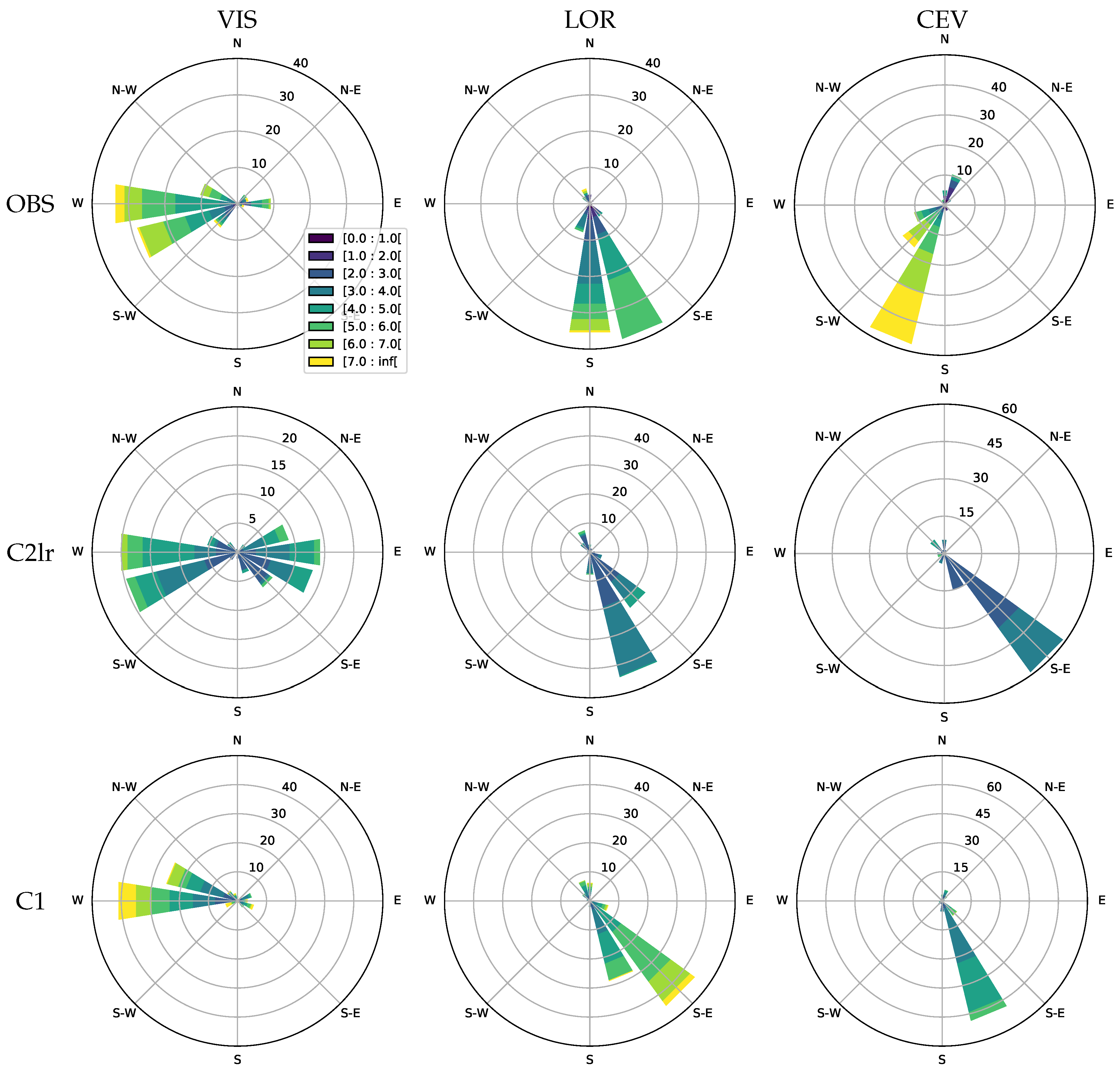
Observed and simulated frequency distribution of the daytime near-surface wind for three typical valleys (large: VIS; medium: LOR; small: CEV) for the evaluation period 10–18 UTC for observations (OBS) and model simulations (C2lr, C1). Bin width is 22.5 and distributions of wind speed are given for each direction (color).
Figure 7.
Observed and simulated frequency distribution of the daytime near-surface wind for three typical valleys (large: VIS; medium: LOR; small: CEV) for the evaluation period 10–18 UTC for observations (OBS) and model simulations (C2lr, C1). Bin width is 22.5 and distributions of wind speed are given for each direction (color).

Figure 8.
Root mean square error (RMSE) of the mean daily maximum valley wind (10–14 UTC) for the four main simulations.
Figure 8.
Root mean square error (RMSE) of the mean daily maximum valley wind (10–14 UTC) for the four main simulations.

Figure 9.
Box plot of the RMSE for the mean daily maximum valley wind (10–14 UTC) for the four main simulations.
Figure 9.
Box plot of the RMSE for the mean daily maximum valley wind (10–14 UTC) for the four main simulations.

Figure 10.
RMSE of the mean daily maximum valley wind (10–14 UTC) versus the altitude bias of the corresponding model grid point.
Figure 10.
RMSE of the mean daily maximum valley wind (10–14 UTC) versus the altitude bias of the corresponding model grid point.

Figure 11.
An assessment of the impact of the three land surface datasets, namely soil type, land cover, and topography, on the simulated mean diurnal cycle of the diurnal valley winds. Box plot of RMSE as in Figure 9. Land surface datasets used, from left to right: (1) all low-resolution; (2) high-resolution soil type; (3) high-resolution land cover; (4) high-resolution soil type and land cover; (5) all high-resolution.

Figure 12.
As in Figure 6, but for three valleys with poor skill for C1; that is for ALT (Altdorf), GLA (Glarus), and CEV (Cevio), see Figure A1.

Figure 13.
Effect of grid resolution and filtering on the topography for a large valley (a) and a small valley (b). The black line denotes the ASTER data interpolated onto a 67 m resolution grid.
Figure 13.
Effect of grid resolution and filtering on the topography for a large valley (a) and a small valley (b). The black line denotes the ASTER data interpolated onto a 67 m resolution grid.

Figure 14.
Effect of resolution and topography filtering on the height of the ridgeline (b,d) and the area–height distribution (e,f) for a large catchment, the Rhone valley (a), and a small catchment, the Maggia valley (c). (a,c) The distance along the circumference of the catchment is marked every 50 km. The axes denote the location in Swiss coordinates (in km). (b,d) The horizontal axis denotes the distance along the circumference of the catchment.


Table 1.
Summary of the main numerical experiments. The abbreviation LSD refers to land surface datasets, slope refers to the maximum slope in the integration domain, and equals the root-mean-square error of the height differences between the diurnal wind stations and the corresponding grid points.
Table 1.
Summary of the main numerical experiments. The abbreviation LSD refers to land surface datasets, slope refers to the maximum slope in the integration domain, and equals the root-mean-square error of the height differences between the diurnal wind stations and the corresponding grid points.
| Experiment | (km) | (s) | LSD | Filter Cutoff | Slope () | (m) |
|---|---|---|---|---|---|---|
| C1 | 1.1 | 10 s | high-res | 5 | 33.2 | 216 |
| C1lr | 1.1 | 10 s | low-res | 5 | 25.3 | 222 |
| C2 | 2.2 | 20 s | high-res | 5 | 20.3 | 378 |
| C2lr | 2.2 | 20 s | low-res | 5 | 20.2 | 348 |
| C1f | 1.1 | 10 s | high-res | 3.5 | 43.6 | 142 |
| C500f | 0.55 | 5 s | high-res | 3.5 | 45.6 | 78 |
Table 2.
Overview of land surface datasets and their resolution used in this study. The abbreviations refer to Advanced Spaceborne Thermal Emission and Reflection Radiometer global digital elevation map (ASTER), Harmonized World Soil Database (HWSD), GlobCover 2009 (GC2009), Global Land One-km Base Elevation project (GLOBE), FAO Digital Soil Map of the World (FAO DSMW), and Global Land Cover 2000 (GLC2000). For further information on these datasets and their use in the COSMO model see [42].
| Characteristic | High-Resolution Datasets | Low-Resolution Datasets |
|---|---|---|
| Topography | ASTER, 30 m | GLOBE, 1 km |
| Soil | HWSD, 1 km | FAO DSMW, 10 km |
| Land cover | GC2009, 300 m | GLC2000, 1 km |
Table 3.
Characterization of diurnal wind stations that are identified in Figure 1b. The last column characterizes the local site of the station. The abbreviation lrgval, medval, and smlval refer to a large valley (lrgval), a medium-sized valley (medval), and a small-valley (smlval), respectively. The typical valley floor width is 2 km, 1 km, and 500 m for the three valley sizes. The valley stations are typically located at the valley floor. The abbreviations junc and curv refer to a station located near a valley junction and in a curve, respectively, lake refers to a lakeshore site, ridge to a station located on a mountain ridge, and pass to a station on a mountain pass.
| Catchment | Acronym | Station | Height (m) | Site |
|---|---|---|---|---|
| Inn | SAM | Samedan | 1708 | medval (junc) |
| Linth | GLA | Glarus | 517 | medval (junc) |
| Reuss | ALT | Altdorf | 438 | lrgval |
| GUE | Guetsch | 2287 | ridge | |
| Rhein | CHU | Chur | 556 | lrgval (curv) |
| CMA | Crap Masegen | 2480 | ridge | |
| PMA | Piz Martegnas | 2670 | ridge | |
| QUI | Quinten | 419 | lake | |
| VAB | Valbella | 1569 | medval | |
| VAD | Vaduz | 457 | lrgval | |
| WFJ | Weissfluhjoch | 2690 | ridge | |
| Rhone | EVI | Evionnaz | 482 | lrgval |
| GRH | Grimsel Hospiz | 1980 | pass | |
| GSB | Col de Grand | 2472 | pass | |
| St. Bernard | ||||
| SIO | Sion | 482 | lrgval | |
| ULR | Ulrichen | 1345 | medval | |
| VIS | Visp | 639 | lrgval | |
| ZER | Zermatt | 1638 | smlval | |
| Ticino | CEV | Cevio | 417 | smlval (curv) |
| LOR | Lodrino | 261 | medval | |
| PIO | Piotta | 990 | smlval |
Table 4.
Model altitude bias (m) for typical stations in large, medium-sized, and small valleys and the mean altitude bias of all diurnal wind stations.
Table 4.
Model altitude bias (m) for typical stations in large, medium-sized, and small valleys and the mean altitude bias of all diurnal wind stations.
| Valley | Station | C2 | C1 | C1f | C500f |
|---|---|---|---|---|---|
| large | VIS | 354 | 158 | 66 | |
| ALT | 334 | 9 | 3 | ||
| medium | LOR | 379 | 188 | 103 | |
| GLA | 459 | 134 | 41 | 3 | |
| small | CEV | 570 | 408 | 230 | 195 |
| PIO | 553 | 344 | 235 | 51 | |
| all | all | 226 | 74 | 28 | 5 |
© 2018 by the authors. Licensee MDPI, Basel, Switzerland. This article is an open access article distributed under the terms and conditions of the Creative Commons Attribution (CC BY) license (http://creativecommons.org/licenses/by/4.0/).
Share and Cite
MDPI and ACS Style
Schmidli, J.; Böing, S.; Fuhrer, O. Accuracy of Simulated Diurnal Valley Winds in the Swiss Alps: Influence of Grid Resolution, Topography Filtering, and Land Surface Datasets. Atmosphere 2018, 9, 196. https://doi.org/10.3390/atmos9050196
AMA Style
Schmidli J, Böing S, Fuhrer O. Accuracy of Simulated Diurnal Valley Winds in the Swiss Alps: Influence of Grid Resolution, Topography Filtering, and Land Surface Datasets. Atmosphere. 2018; 9(5):196. https://doi.org/10.3390/atmos9050196
Chicago/Turabian StyleSchmidli, Juerg, Steven Böing, and Oliver Fuhrer. 2018. "Accuracy of Simulated Diurnal Valley Winds in the Swiss Alps: Influence of Grid Resolution, Topography Filtering, and Land Surface Datasets" Atmosphere 9, no. 5: 196. https://doi.org/10.3390/atmos9050196
Note that from the first issue of 2016, this journal uses article numbers instead of page numbers. See further details here.