Analysis of Compositional Variation and Source Characteristics of Water-Soluble Ions in PM_2.5 during Several Winter-Haze Pollution Episodes in Shenyang, China

Abstract

From 18 February to 13 March 2014 and from 17 December 2016 to 27 January 2017, an online analyzer for monitoring aerosols and gases (MARGA) and an online single particle aerosol mass spectrometer (SPAMS) were used to measure and analyze the concentrations and sources of water-soluble (WS) ions in PM₁₀, PM_2.5, and gases (NH₃, HNO₃, HCl), in Shenyang City, China. During the field campaign, nine haze episodes (or smog episodes, total 582 h) were identified, with 960 identified as non-haze periods. The average mass concentrations of PM_2.5 and total water-soluble ions (TWSIs) in PM_2.5 during haze episodes were 131 μg·m⁻³ and 77.2 μg·m⁻³, 2.3 times and 1.9 times the values in non-haze periods, respectively. The average mass concentration of TWSIs in PM_2.5 was 55.9 μg·m⁻³ (accounting for 55.9% of PM_2.5 mass loading), 37.6% of which was sulfate, 31.7% nitrate, 20.0% ammonium, 6.6% chloride, 1.9% potassium, 1.4% calcium, and 0.8% magnesium throughout the campaign. Concentrations of sulfate, nitrate, and ammonium (SNA) secondary pollution ions increased rapidly during haze episodes to as much as 2.2 times, 3.0 times, and 2.4 times higher than during non-haze periods, respectively. Diurnal variations during non-haze periods were significant, while complex pollution was insignificant. Based on changes in the backward trajectories and concentrations of WS ions, the hazy episodes were divided into three types: complex, coal-burning, and automobile exhaust pollution. All complex episodes had high concentrations and greater contributions of ammonium nitrate from complex and automobile exhaust pollution, while the contribution of ammonium sulfate from coal-burning pollution was greater than that of ammonium nitrate. The correlation coefficients among SNA species were very high in complex pollution, with nitrate and sulfate the main forms present. The results of principal component analysis (PCA) were related to emissions from burning coal for heating and from long-range transmission in winter. In the case of exhaust pollution, NO₃⁻ accounted for the highest percentage of PM_2.5, and NH₄⁺ was more closely related to NO₃⁻ than to SO₄²⁻. Coal-burning pollution was the most common type of pollution in Shenyang. The contribution of sulfate was higher than that of nitrate. Based on PCA, the contribution of coal-burning emissions varied from 36.7% to 53.6% due to industry, soil sources, and other factors.

1. Introduction

In recent years, Northeast China has suffered from serious atmospheric particulate pollution. In autumn and winter especially, the northeastern region exhibits the earliest and most serious haze pollution of all areas of China, which causes major harm to the health of local residents. During this period, there is explosive growth of haze pollution due to emissions from the combustion of coal and straw for heating, as well as a weather pattern that is not conducive to dispersal [1]. In addition, in Northeast China the winter heating period is long and the inversion layer exists for a long period, making the impact of coal-burning pollution even greater [2]. Combined emissions from coal-fired power plants, automotive exhaust, and various industries cause atmospheric particulates there to reach higher concentrations and have more complex components [3]. The chemical composition of these particulates varies greatly among regions. As previous studies of water-soluble (WS) ions in the region are quite limited and existing studies mostly employed off-line sampling methods without adequate temporal resolution, it is essential to study the characteristics and sources of PM_2.5 and its water-soluble ions in Northeast China during various pollution episodes.

Atmospheric particulates often consist of multiple chemical components and may have extremely complex compositions. Particles interact with solar radiation by absorbing and scattering light, creating a haze that reduces atmospheric visibility. As this affects the Earth’s climate system, it has prompted intense research in this area [4]. In addition to the concentrations of water-soluble (WS) ions, the size of a particle also determines its pH, which affects the gas-particle partitioning of semi-volatile compounds [5]. Furthermore, changes in particle concentrations are directly associated with the occurrence of haze [6]. During haze episodes under high humidity conditions, liquid phase reactions play a key role in the formation of secondary particles in PM₁ (submicron aerosol, with an aerodynamic diameter less than 1.0 μm). Secondary particles absorb water due to their hydrophilicity, which causes them to increase in size and mass concentration, enhancing the efficiency of radiation scattering [7]. The principal components of secondary particles are the secondary ions SO₄²⁻, NO₃⁻, and NH₄⁺ (SNA) and organic compounds [8]. Secondary particles are formed mainly from gas precursors (such as SO₂, NO_x, NH₃, etc.) through chemical reactions in the atmosphere [9]. The composition of secondary particles across different regions is diverse. For example, in the western United States, specifically California, secondary particles exist in a mixed form as NH₄NO₃, NH₄HSO₄, and (NH₄)₂SO₄ [10]. In contrast, in northwest Europe, NH₄NO₃ is the primary form of ammonium salts [11], e.g., in Germany [12], France [13], Britain [14], and the Netherlands [15]. In China, the principal forms of ammonium salts in urban particles are ammonium sulfate and ammonium nitrate [16]. Once ammonium sulfate is formed, it is able to exist in a steady state, whereas ammonium nitrate is unstable in the atmosphere and exists in a state of chemical equilibrium together with gaseous ammonia (NH₃) and nitric acid (HNO₃) [17]. During periods characterized by complex pollution caused by biomass burning and secondary aerosols in Shanghai, concentrations of ions (e.g., sulfate and nitrate) rose significantly due to heterogeneous reactions between SO₂ and NO₂ on the surface of pre-existing KCl particles [18]. The formation of ammonium sulfate and nitrate depends directly on the gaseous ammonia available. Ammonia combines with sulfuric acid and nitric acid in a competitive manner to form ammonium nitrate and ammonium sulfate, respectively [12]. During the summer in Beijing and Shanghai, nitrate formation is related to both relative humidity and particle concentrations; specifically, N₂O₅ is hydrolyzed through heterogeneous reactions on the surface of aqueous acidic particles to form nitrate. Nitrate formation in Lanzhou and Guangzhou is mainly completed by gas-phase reactions under NH₃-rich conditions [19].

Furthermore, such studies have rarely been performed in northeastern China. Therefore, it is important to study the characteristics and sources of WS ions in PM_2.5 on winter haze days in Shenyang, the central city of northeastern China. In this study, online observations and source apportionment were used to analyze the physical and chemical features of WS ions in Shenyang, as well as their correlations, on days with various levels of haze pollution. The formation of these ions with respect to pollution formation is discussed, and an analysis of the pollution sources is presented.

2. Experiments

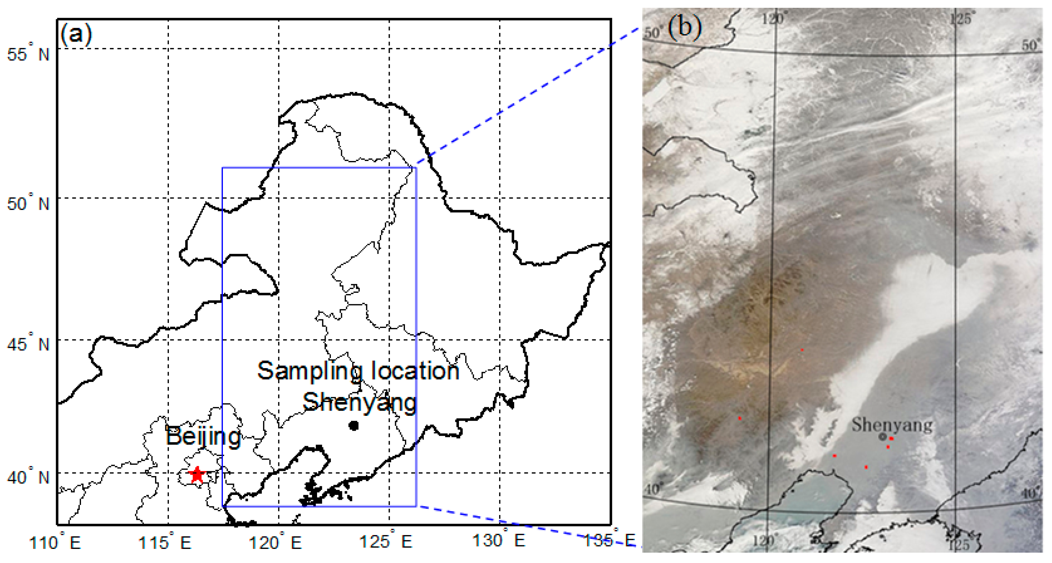
2.1. Sampling and Analysis

In this study, observations were made from the Shenyang Atmospheric Composition Monitoring Station (123°24′44′′ E, 41°43′53′′ N, see Figure 1), situated southwest of the Shenyang urban area. Ambient air was sampled at about 60 m above the ground on the top of a 20-story building belonging to the Northeastern Regional Meteorological Center (Figure 1). The site is located downwind of the prevailing wind that passes over Shenyang, with no obvious large-scale air-pollution sources in its vicinity other than buildings and road dust.

In this study, mass concentrations of PM₁₀, PM_2.5, SO₂, and NO₂ were acquired from data provided by the Liaoning real-time air quality publishing system (http://211.137.19.74:8089 /Home/RealTime). WS ion components in PM₁₀ (PM_2.5) were measured using monitoring of aerosols and gases (MARGA) at 60-min resolution. Measured species included Cl⁻, NO₃⁻, SO₄²⁻, NH₄⁺, Na⁺, K⁺, Ca²⁺, and Mg²⁺, with lower detection limits of 0.01, 0.05, 0.04, 0.05, 0.05, 0.09, 0.10, and 0.06 μg·m⁻³, respectively. During the observation period, only a few water-soluble ions had concentrations below the detection limit, while all others were above it, indicating that the measured results were accurate. Nearly 200 Na⁺ observations fell below the detection limit and were therefore not analyzed. The source apportionment instrument used for this study was an online single-particle aerosol mass spectrometer (SPAMS, HeXin, Guangzhou, China), with measurements made over a particle diameter range of 200 nm to 2.0 μm at a resolution of 500; the mass spectrometer measurement range was ±250 at the maximum m/z. Additionally, several meteorological parameters were measured: atmospheric visibility, humidity, temperature, wind direction, and wind speed. The ambient observation periods were 18 February to 13 March 2014 and 17 December 2016 to 27 January 2017.

2.2. Operating Principles of Observation Instruments

2.2.1. MARGA Operating Principle and Data Analysis

The MARGA instrument, (ADI 2080, Applikon Analytical B.V., Delft, The Netherlands), with a PM₁₀ (PM_2.5) sharp-cut cyclone, was used to obtain an hourly integrated dataset of both inorganic aerosol composition components (NH₄⁺, Na⁺, K⁺, Ca²⁺, Mg²⁺, SO₄²⁻, NO₃⁻, Cl⁻) and their precursor gas concentrations (HCl, HONO, SO₂, HNO₃, NH₃). MARGA consists of both sampling and analytical modules [20]. The two most important components in the sampling module are a wet rotating denuder (WRD) for precursor gas collection and a steam jet aerosol collector (SJAC) for the collection of particulate matter PM₁₀ (PM_2.5) [21]. To track changes in retention time and detector response, this instrument was subject to continuous internal calibration over the entire observation period, by applying a method that uses bromide for the anion chromatogram and lithium for the cation chromatogram. Full details of the MARGA instrument are provided elsewhere [22]. The operation and maintenance of the MARGA instrument was performed according to the manufacturer’s instructions.

2.2.2. Online Single Particle Aerosol Mass Spectrometer (SPAMS 5)

In this study, a single-particle aerosol mass spectrometer (SPAMS) was employed during the winter of 2014 in urban Shenyang to determine both the size and chemical composition of individual atmospheric particles, using a vacuum aerodynamic diameter (d_va) in the size range 0.2–2 lm. During the observation period, 14,516,615 particulate samples were obtained, with mass spectral information collected for 4,049,568. The method for particle collection by the SPAMS instrument was previously described in full by Li et al. [23]. Briefly, particles are first dried using a sequential 30-cm diffusion dryer filled with silica gel, before being introduced into SPAMS through a critical orifice. The particles are then focused and accelerated to specific velocities, determined by their time of flight through two continuous diode Nd: YAG laser beams (wavelength: 532 nm) in the sizing region. The particles are subsequently desorbed and ionized using a pulsed laser (wavelength: 266 nm), which is triggered based on the exact velocity of a specific particle. The positive and negative fragments generated are recorded with D_va. Particle mass spectra were imported into MATLAB (Math Works Inc., Natick, MA, USA) and analyzed using YAADA (V2.1, http://www.yaada.org). Individual particles were classified into different groups or clusters, using ART-2a [24], based on the similarity of mass spectra (presence and intensity of ions) with a vigilance factor of 0.7, a learning rate of 0.05, and 20 iterations [25]. Using ART-2a, eight classes of particles present on haze days were distinguished: dust, organic carbon (OC), elemental carbon (EC), internally mixed organics and elemental carbon (ECOC), high-molecular-weight OC (HMOC), K-rich, inorganic Na-K, inorganic particles, and heavy metals.

Source apportionment of particulates was conducted to obtain the emission-source spectrum of Shenyang; sampling was conducted on the basis of the local industry/energy structure [26]. Based on the observed results of SPAMS described above, and in accordance with the proposed technical guidelines for atmospheric particulate source apportionment [27] and the source spectral library of atmospheric pollutant emissions in Shenyang, the main sources were distinguished and analyzed. The sources of fine atmospheric particulates in Shenyang were divided into seven categories: coal-burning, industrial processes (non-combustion), mobile exhaust gas, dust, biomass combustion, pure secondary inorganic sources, and other sources (Figure 2).

3. Results and Discussion

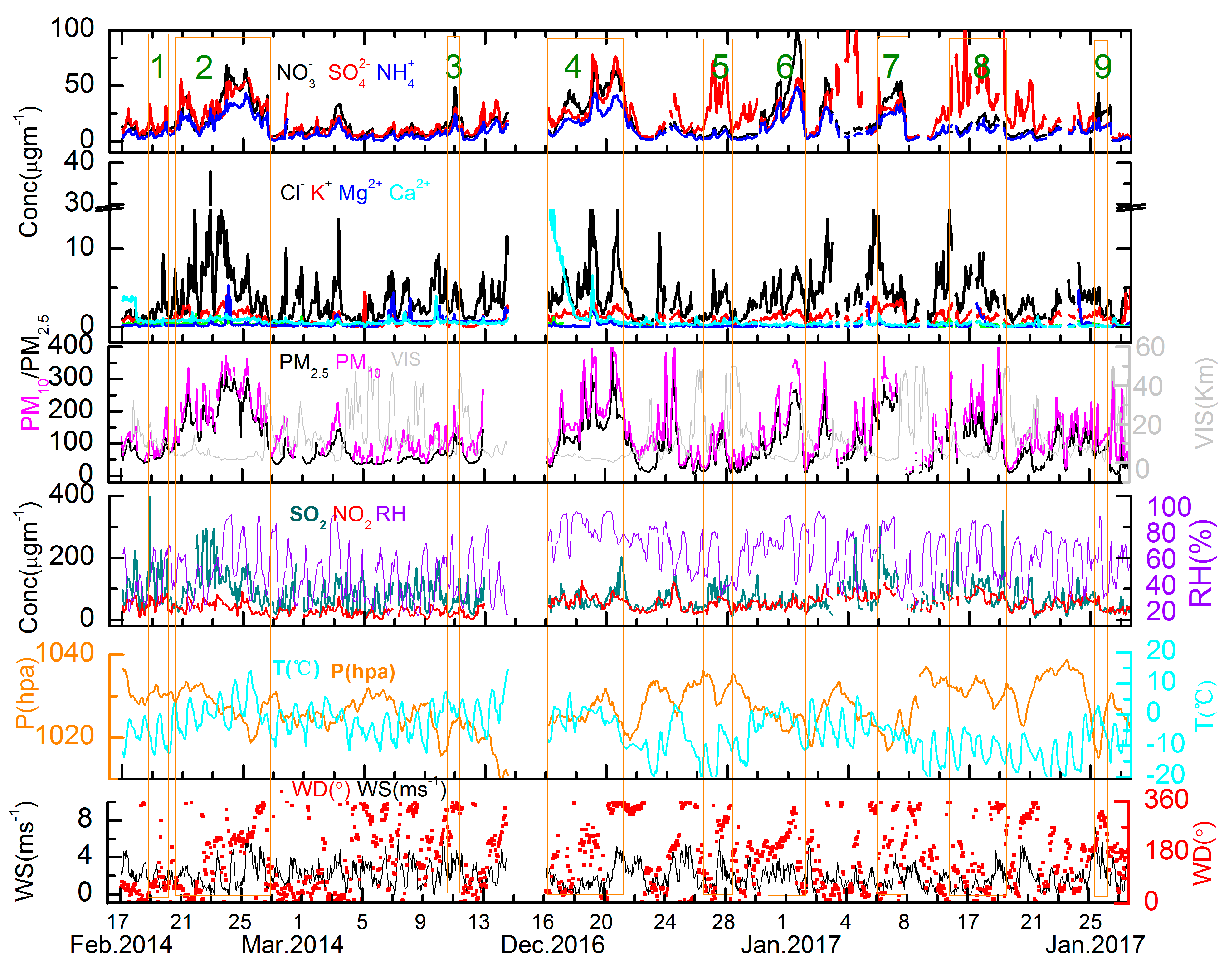
3.1. Haze Pollution Episodes

The principal components of atmospheric particulates were the water-soluble ions SO₄²⁻, NO₃⁻, NH₄⁺, K⁺, Cl⁻, Mg²⁺, and Ca²⁺. Figure 3 shows a time series of atmospheric visibility (Vis, km), relative humidity (RH, %), temperature (°C), wind direction, wind speed (m·s⁻¹), and hourly concentrations of PM₁₀, PM_2.5, and TWSIs measured over the ambient observation period. According to “Haze Observation and Forecast Level” [28], atmospheric conditions where Vis < 10 km may be defined as haze when RH < 80% and as fog when RH > 95%. For RH values between 80% and 95%, atmospheric conditions are defined as a fog-haze blend, which requires further classification according to PM concentrations or surface observation standards. Nine haze episodes (total 582 h) were identified during the campaign in Shenyang (denoted by shaded sequences in Figure 3). As pollution episodes 2, 4, 7, 8, and 9 were associated with high RH, we describe them as smog pollution episodes. The remaining 960 h were identified as non-haze periods.

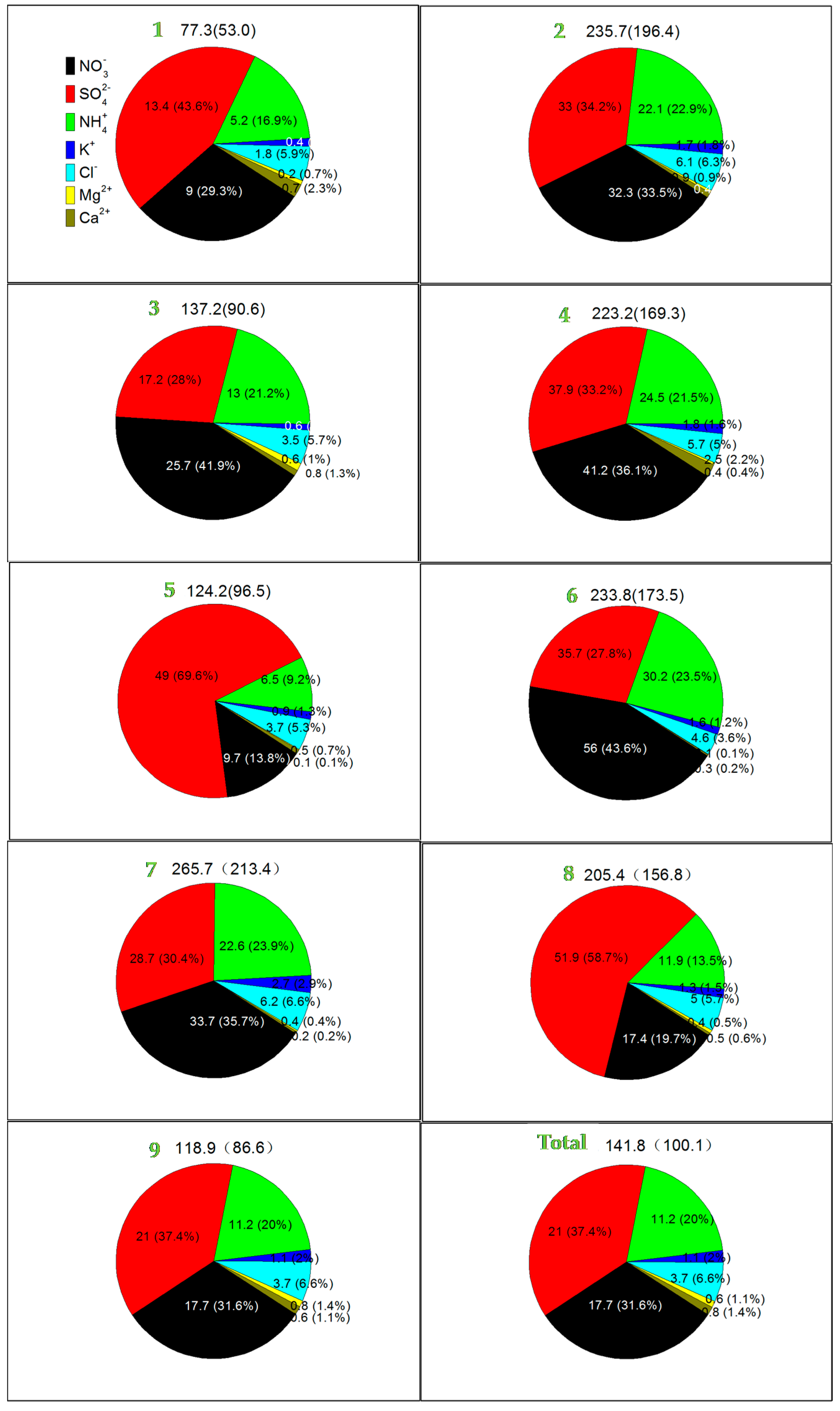
3.2. Water-Soluble Ion Components in Atmospheric Particulates

Table 1. Comparison of the average concentrations (μg·m⁻³) of TWSIs ions among different cities on haze episodes and non-haze period.

PM	Start and End Time/Location & Reference	Weather	NO3−	SO42−	NH4+	K+	Cl−	Mg2+	Ca2+	TWSI	SNA/PM2.5	Sample Mode
PM10	1. 19 February 2014 03:00–20 February 2014 03:00, This study	Haze	9	13.4	5.2	0.4	1.8	0.2	0.7	30.7	52.1	Marga 1s
	2. 20 February 22: 00–27 February 2014 02:00, This study	-	32.3	33.0	22.1	1.7	6.1	0.4	0.9	96.7	44.6	-
	3. 11 March 2014 03:00–11 March 2014 22:00, This study	-	25.6	17.2	12.9	0.6	3.5	0.8	0.6	61.2	61.5	-
PM2.5	4. 17 December 2016 00:00–21 December 2016 14:00, This study	Haze	41.2	37.9	24.5	1.8	5.7	0.4	2.5	114	61.2	Marga 1s
	5. 27 December 2016 06:00–28 December 2016 08:00, This study	-	9.7	49	6.5	0.9	3.7	0.1	0.5	70.4	67.6	-
	6. 31 December 2016 08:00–02 January 2017 08:00, This study	-	56	35.7	30.2	1.6	4.6	0.1	0.3	129	70.3	-
	7. 06 January 2017 23:00–09 January 2017 02:00, This study	-	33.7	28.7	22.6	2.7	6.2	0.2	0.4	94.5	39.8	-
	8. 16 January 2017 22:00–19 January 2017 15:00, This study	-	17.4	51.9	11.9	1.3	5	0.5	0.4	88.4	52.0	-
	9. 25 January 2017 14:00–26 January 2017 15:00, This study	-	26.8	14.5	13.9	1.3	2.9	0.1	0.1	59.6	63.7	-
PM10	18 February to 15 March 2014, This study	Haze average	22.3	21.2	13.4	0.9	3.8	0.5	0.7	62.8	50.3	Marga 1s
		Non-haze average	10.4	11.7	7.0	0.9	3.4	0.7	0.7	34.7	34.6
		average	16.3	16.5	10.2	0.9	3.6	0.6	0.7	48.8	43.6
PM2.5	17 December 2016 to 27 January 2017, This study	Haze average	30.8	36.3	18.3	1.6	4.7	0.2	0.7	92.6	57.2
		Non-haze average	7.4	14.9	6.0	0.8	3.0	0.4	1.0	33.5	52.4
		average	19.1	25.6	12.1	1.2	3.8	0.3	0.9	63.0	55.9
PM10 and PM2.5	18 February to 15 March 2014 and 17 December 2016 to 27 January 2017, This study	Haze average	26.6	28.7	15.8	1.3	4.2	0.4	0.7	77.7	54.2	Marga 1s
		Non-haze average	8.9	13.3	6.5	0.9	3.2	0.5	0.8	34.1	41.6
		average	17.7	21.0	11.2	1.1	3.7	0.5	0.8	55.9	49.9
PM10	5 January to 5 February 2012, Beijing, China [37]	-	22.7	38.9	22.4	2.7	6.5	0.2	0.8	94.2	-	Teflon filter
	December 2011, Delhi, India [29]	-	16.4	13.3	9.4	1.8	6.2	0.7	4.4	52.2	-	Quartz filters
	December 2011, Varanasi, India [29]	-	16.7	16.7	7.8	2	9.6	0.8	4.3	57.9	-	Quartz filters
	December 2011, Kolkata, India [29]	-	7	13.5	8.3	5.1	13.6	1	7.3	55.8	-	Quartz filters
PM2.5	Cold seasons, 2003, Milan, Italy [30]	-	15.2	5.3	4.5	NA	0.7	NA	NA	25.7	-	Quartz filters
	2000–2003, New York, NY, USA [31]	Annual average	2	4.3	1.9	0.1	0.1	NA	NA	8.4	-	Quartz filters
	Winter, 2005–2006, Lahore, Pakistan [32]	Fog	18.9	19.2	16.1	3.5	7.4	0.08	0.89	66.1	-	Quartz filters
	October to March 2010–2012, Guangzhou, China [36]	Haze	8.2	12.8	10.1	0.3	2	0.1	0.3	33.8	-	Marga 1s
	25 January to 3 February 2013, Nanjing, China [34]	Haze	13	32.6	20.4	1.1	0.5	0.2	2.2	70	-	Quartz filters
	25 January to 3 February 2013, Nanjing, China [34]	Non-haze	2	12.9	4.7	0.8	0.4	0.2	1.9	22.9	-	Quartz filters
	9–20 January 2013, Wuhan, China [40]	Haze	39.2	38.3	22.8	2.3	2.9	0.2	2.5	108	-	Quartz filters
	Normal, 9–20 January 2013, Wuhan, China [40]	-	12	10.4	7.2	0.6	1.9	0.1	0.4	32.6	-	Quartz filters
	6–18 February 2012, Zhengzhou, China [38]	-	30.1	26	14.3	2.7	8.1	0.3	1.7	83.2	-	Quartz filters
	6–18 February 2012, Luoyang, China [38]	-	18.6	18.5	10.7	1.7	5.1	0.2	0.8	55.6	-	Quartz filters
	6–18 February 2012, Pingdingshan, China [38]	-	29.8	25.6	13.6	2.3	7	0.2	0.6	79.1	-	Quartz filters
	Winter, March 2014 to February 2015, Beijing, China [39]	-	11.2	9.3	5.6	1	2.9	0.1	0.5	30.6	-	Quartz filters
	Winter, 2009–2010, Taiyuan, China [41]	-	13.7	57.2	19.6	2.5	13.5	1	1.4	109	-	Quartz filters
	24 January to 21 February 2014, Nanjing, China [35]	-	5.9	5.1	4.8	0.9	0.9	0.1	0.2	17.9	-	Quartz filters

provides a comparison of the average concentrations (μg·m⁻³) of WS ions at different cities during haze episodes and the non-haze period. The average mass concentration of PM₁₀ (PM_2.5) and TWSIs in PM₁₀ (PM_2.5) in haze episodes were 131 μg·m⁻³ and 77.2 μg·m⁻³, 2.3 times and 1.9 times as those in non-haze periods, respectively (see Table 1 and Figure 3). The average mass concentration of TWSIs in PM_2.5 was 55.9 μg·m⁻³, 37.6% of which was sulfate, 31.7% nitrate, 20.0% ammonium, 6.6% chloride, 1.9% potassium, 1.4% calcium, and 0.8% magnesium in the whole campaign. Concentrations of the secondary pollution ions SO₄²⁻, NO₃⁻, and NH₄⁺ (SNA) increased rapidly during haze episodes, reaching 2.2, 3.0, and 2.4 times levels in non-haze periods, respectively. WS ions accounted for 55.9% of PM_2.5, identical to the 55.9% value observed in Shanghai [18]. The average ion concentration (77.2 μg·m⁻³) of PM_2.5 was higher in Shenyang than in Delhi and Kolkata in India [29]; Milan in Italy [30]; New York in the USA [31]; Lahore in Pakistan [32]; Suzhou [33], Nanjing in winter 2013 and 2014 [34,35], Guangzhou [36], Beijing [37], and Luoyang [38] in China. On the other hand, it was lower than previous measurements in Varanasi in India [29], Beijing in 2015 [39], Wuhan [40], Taiyuan [41], Zhengzhou, and Pingdingshan [38].

WS ions from various sources can be classified into three types: natural (Mg²⁺ and Ca²⁺), secondary (e.g., SO₄²⁻, NO₃⁻, NH₄⁺, SNA), and combustion (K⁺ and Cl⁻) sources [18]. On average, the proportions of ions from natural, secondary, and combustion sources were 1.3, 91.6, and 7.1%, respectively, during the nine haze episodes, and 1.4, 84.1, and 11.9% during the non-haze periods (Table 1). For the combustion-sourced ions K⁺ and Cl⁻, the respective concentrations were 1.4 and 1.3 times higher during haze episodes than in non-haze periods. Concentrations of the natural ions Mg²⁺ and Ca²⁺ were also higher in non-haze periods than during hazy episodes. Concentration of secondary pollution ions SO₄²⁻, NO₃⁻, and NH₄⁺ in nine hazy episodes rose rapidly to 28.7, 26.6, and 15.8 μg·m⁻³, respectively, 2.2, 3.0, and 2.4 times higher, respectively, then the levels observed on non-haze periods.

The SNA fractions in PM_2.5 were 52.1, 44.6, 61.5, 61.2, 67.6, 70.3, 39.8, 52.0, and 63.7% during the nine haze episodes, respectively; 49.9% over the whole period, and 41.6% in non-haze intervals. These results show that SNA were the principal components of PM_2.5 during haze episodes. The SNA fraction (49.9%) was lower than observed in Beijing (55%), but higher than in Shanghai (40%), Lanzhou (26%), and Guangzhou (42%) [25]. These findings indicate that the rise in PM_2.5 concentrations in Shenyang was primarily caused by increased SNA, suggesting that SNA play a key role in haze formation.

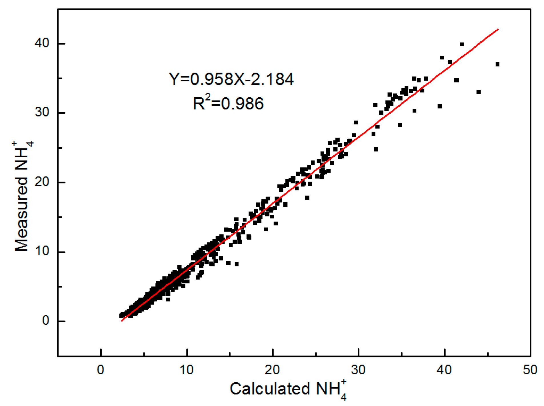
3.3. Neutrality of Water-Soluble Ions

The following equation can be used to estimate whether PM₁₀ is in a neutral state [42]

NH₄⁺_pred = 18 × (2 × (SO₄²⁻)/96 + (NO₃⁻)/62 + (Cl⁻)/35.5)

where SO₄²⁻, NO₃⁻, and NH₄⁺ are the mass concentrations (μg·m⁻³) of each species divided by their molecular weights; 18 is the molecular weight of NH₄⁺. It should be noted that in this equation negative ions are assumed to be neutralized completely by NH₄⁺; hence, the resultant salts are ammonium nitrate, ammonium sulfate, and ammonium chloride. Additionally, metal cations and organic acids are neglected. In this study, the concentrations of other ions were extremely low compared with those of SO₄²⁻, NO₃⁻, and NH₄⁺; thus, the use of this equation is valid. If the calculated value is similar to the observed value, then this indicates that PM₁₀ exists in a neutral state, while higher calculated values suggest it is acidic. In Figure 4, it can be seen that the calculated NH₄⁺ concentrations were equal to the observations, with a slope of 0.986. This indicates that the WS ions in PM₁₀ in Shenyang air exhibited a state of neutrality.

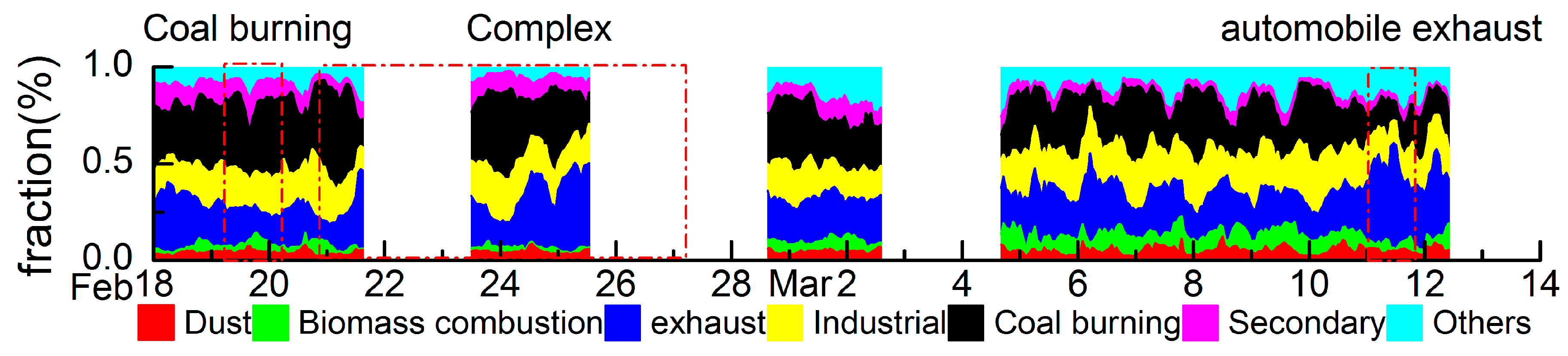
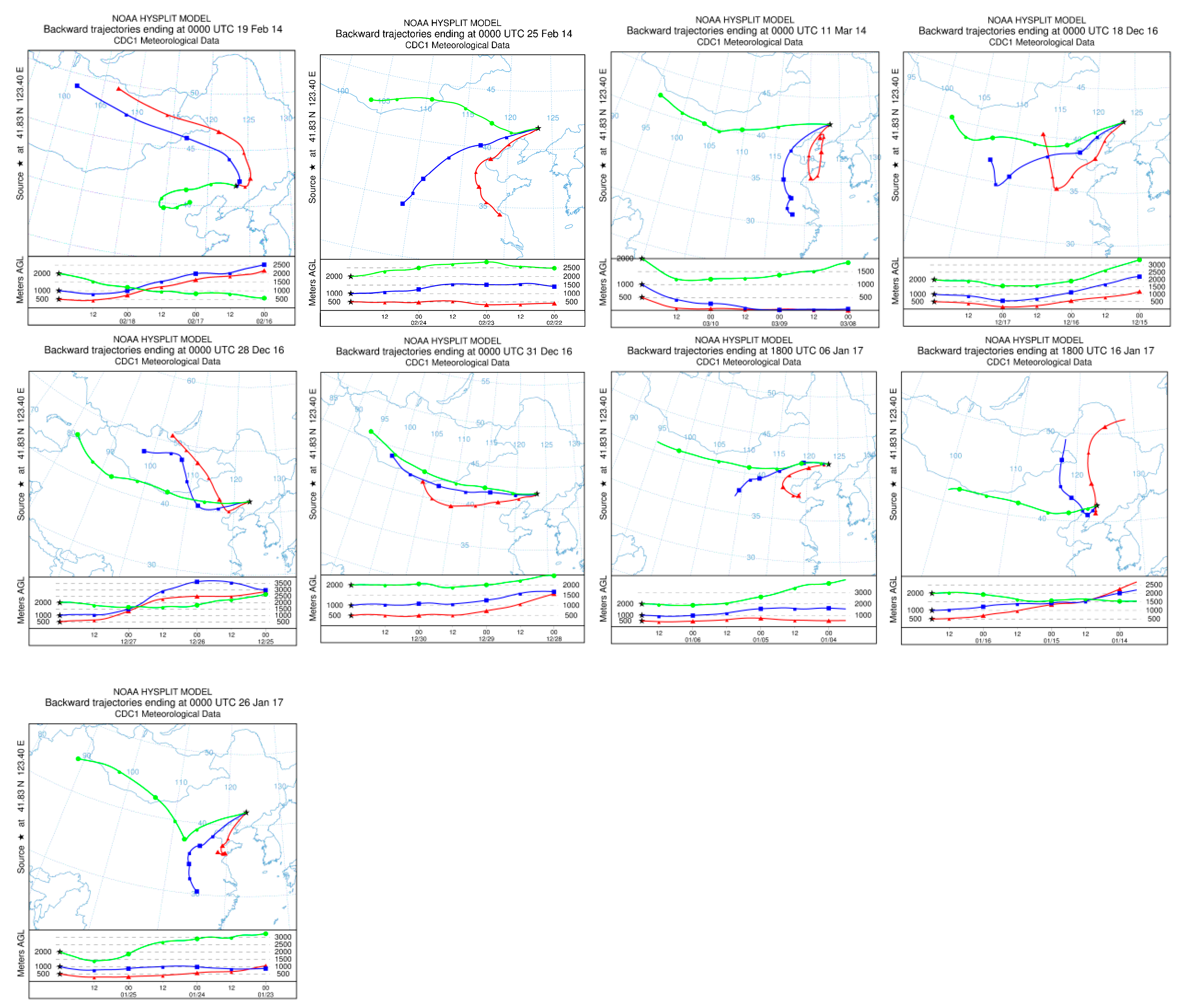
3.4. Variation of Concentration, Existence Patterns, and Sources of Water-Soluble Ions in Different Haze Episodes

Based on changes in the directions of the air masses in the backward trajectories (Figure 5) and the concentrations of water-soluble ions, the nine pollution episodes during the study period can be classified into three categories. Based on the ground surface wind direction in the 72-h backward trajectory, the episodes can be divided into southwesterly and northwesterly directions; the air masses at altitudes of 500 m and 1000 m (represented by the red and blue lines, respectively) of six pollution episodes—2, 3, 4, 6, 7, and 9—came mainly from the southwest, while the air masses of 1, 5, and 8 arrived mainly from the northwest. The pollution episodes with southwesterly flow near the ground surface can be divided into two categories based on duration (Table 1 and

Table 2. Summary of mass concentrations of PM₁₀ and PM_2.5 and their water-soluble ion (µg·m⁻³), gaseous pollutants (µg·m⁻³; mg·m⁻³ for CO), and meteorological parameters during the nine pollution episodes (year of 2014, 2016–2017) and the entire study period, as well as source apportionment fraction (%) based on SPAMS for the 2014 study period.

Air Mass	1. Northwesterly	2. Southwesterly	3. Southwesterly	4. Southwesterly	5. Northwesterly	6. Southwesterly	7. Southwesterly	8. Northwesterly	9. Southwesterly	2014	2016–2017	Total
Source	Coal-Burning	Complex	Automobile Exhaust	Complex	Coal-Burning	Complex	Complex	Coal-Burning	Automobile Exhaust
Episodes	19 February 2014 3:00–20 February 2014 3:00	20 February 2014 22:00–27 February 2014 2:00	11 March 2014 3:00–11 March 2014 22:00	17 December 2016 0:00–21 December 2016 14:00	27 December 2016 6:00–28 December 2016 8:00	31 December 2016 8:00 –2 January 2017 8:00	6 January 2017 23: 00–9 January 2017 2:00	16 January 2017 22: 00–19 January 2017 15:00	25 January 2017 14:00–26 January 2017 15:00
PM2.5	53.0	196	90.6	169	96.5	174	213	156	86.6	113	149	131
PM10	77.3	236	137	223	124	234	266	205	119	150	195	173
NO3−	9.0	32.3	25.7	41.2	9.7	56.0	33.7	17.4	26.8	22.3	30.8	26.6
SO42+	13.4	33.0	17.2	37.9	49.0	35.7	28.7	51.9	14.5	21.2	36.3	28.7
NH4+	5.2	22.1	13.0	24.5	6.5	30.2	22.6	11.9	13.9	13.4	18.3	15.8
K+	0.4	1.7	0.6	1.8	0.9	1.6	2.7	1.3	1.3	0.9	1.6	1.3
Cl−	1.8	6.1	3.5	5.7	3.7	4.6	6.2	5.0	2.9	3.8	4.7	4.2
Mg2+	0.2	0.4	0.8	0.4	0.1	0.1	0.2	0.5	0.1	0.5	0.3	0.4
Ca2+	0.7	0.9	0.6	2.5	0.5	0.3	0.4	0.4	0.1	0.7	0.7	0.7
TWSIs	31.3	97.1	61.2	114	70.3	129	94.6	68.5	59.7	63.2	89.3	76.3
Percentage	40.5	41.2	44.6	67.4	72.9	74.1	44.3	43.9	69.0	42.1	61.9	52.0
AQI	74	242	120	215	128	219	263	200	115	145	190	168
SO2	155.4	119.0	62.4	71.6	95.9	54.4	132	101	40.3	112	82.5	97.4
NO2	56.1	43.7	21.9	67.6	62.6	49.3	92.1	78.9	40.5	40.6	65.2	52.9
CO	0.8	1.9	1.2	2.2	1.5	2.1	2.1	2.1	1.8	1.3	2.0	1.6
O3	45.0	43.6	59.7	17.7	9.5	30.8	4.5	7.1	64.5	49.4	22.3	35.9
HCl	0.1	0.2	0.5	0.1	0.4	0.2	0.4	0.7	0.3	0.3	0.4	0.3
HNO2	0.2	0.8	1.0	1.1	0.6	1.0	0.9	1.2	1.0	0.7	1.0	0.8
HNO3	2.8	3.3	2.4	1.3	2.6	1.0	1.8	3.2	1.2	2.8	1.8	2.3
NH3	0.9	5.9	9.1	3.8	0.4	3.3	3.4	2.0	4.7	5.3	2.9	4.1
P	1031	1028	1024	1026	1030	1024	1021	1031	1023	1027	1026	1027
T	−6.0	1.5	1.8	−1.1	−11.5	−1.3	−4.9	−10.3	−4.2	−0.9	−5.5	−3.2
RH	43.8	55.3	43.5	86.4	58.3	75.1	67.8	66.3	57.0	47.5	68.5	58.0
WS	2.0	2.1	3.2	1.5	2.2	2.2	1.7	1.4	3.6	2.4	2.1	2.3
VIS	10,995	4988	16,802	2601	14,515	5481	8547	7335	7076	10,929	7592	9261
Sand	5	4	5	-	-	-	-	-	-	-	-	-
Combustion	4	2	4	-	-	-	-	-	-	-	-	-
Vehicle	18	26	38	-	-	-	-	-	-	-	-	-
Industry	19	19	15	-	-	-	-	-	-	-	-	-
Coal	35	34	16	-	-	-	-	-	-	-	-	-
Secondary	11	8	4	-	-	-	-	-	-	-	-	-
Others	8	6	17	-	-	-	-	-	-	-	-	-

). The episodes with long hazy periods were Episodes 2, 4, 6, and 7. During this type of pollution episode, the concentrations of SO₄²⁻, NO₃⁻, and NH₄⁺ in water-soluble ions all had peak values. The NH₃ content, with its strong atmospheric oxidation ability, was highest, which signifies that atmospheric particulates formed rapidly and in a complex manner. In this paper, the SPAMS source-apportionment results for mixed pollutants (Figure 2, 22 February 2014 16:00–27 February 2014 02:00) indicate that coal burning accounted for 31% and automobile exhaust for 28% (Figure 2, Table 2). In total, these two sources accounted for nearly 60%. Therefore, this period was classified as complex pollution.

In pollution Episodes 3 and 9, the duration of pollution was short, yet NO₃⁻ concentrations increased rapidly. As the percentage of automobile exhaust in SPAMS source-apportionment was 38% and coal burning accounted for only 20% (Figure 2, Table 2), pollution Episodes 3 and 9 were classified as automobile exhaust pollution.

Among the coal-burning pollution episodes, the air masses at altitudes of 500 m and 1000 m came mainly from the northwest in pollution Episodes 1, 5, and 8 (Figure 5), with rapid increases in SO₄²⁻ concentrations. Based on the SPAMS source-apportionment results for pollution Episode 1, coal burning accounted for as much as 40% while automobile exhaust accounted for only 20% (Figure 2, Table 2). Therefore, these pollution episodes are collectively referred to as coal-burning pollution. This paper provides analysis of the characteristics, presence patterns, and sources of water-soluble ions collected during these nine pollution episodes.

Figure 6 shows the concentrations (µg·m⁻³) and mass fractions (%) of each aerosol species in TWSIs during pollution Episodes 1–9 (upper part of the figure shows the concentrations of PM₁₀ and PM_2.5 during these episodes in parentheses) and the entire study period. As shown in Figure 6 and Table 2, concentrations were very high during all complex-pollution episodes; concentrations of PM₁₀ (PM_2.5) in Episodes 2, 4, 6, and 7 were as high as 236 (197), 223 (169), 234 (174), and 266 (213) μg·m⁻³. The concentrations of NO₃⁻ ranged from 32.3 μg·m⁻³ to 56 μg·m⁻³, with the percentage of TWSIs ranging from 33.3% to 43.6%. These concentrations are the highest among all pollution episodes, with percentages that are lower only than those of automobile exhaust pollution. The concentration of NO₃⁻ in automobile exhaust pollution Episode 3 and 9 were 25.7 μg·m⁻³ and 26.8 μg·m⁻³, respectively, accounting for 41.9% and 44.9% in TWSIs respectively, which is the highest among all pollution episodes. The concentration of SO₄²⁻ in coal-burning pollution Episode 1, 5, and 8 was 13.4 (accounting for 42.7% of TWSIs), 49 (69.6%), and 52.0 μg·m⁻³ (58.6%), much higher than NO₃⁻ at 9.0 (28.7%), 9.7 (13.8%), and 17.4 μg·m⁻³ (19.6%). Higher concentrations and percentages of SO₄²⁻ than of NO₃⁻ are common features of coal-burning pollution.

3.4.1. Complex Pollution

Pollution Episodes 2, 4, 6, and 7 were both of the complex-pollution type. The complex-pollution episodes were the most serious, with the highest concentrations of particles, longest durations, and concentrations of nitrate higher than (or similar to) those of sulfate. Their common features were low sea-level pressure, high temperature, low wind speed, high relative humidity, and southerly winds at the ground surface (Figure 3 and Table 2). Thus, complex pollution was the result of explosive growth of atmospheric particulate matter under the control of weak low-pressure fields on the ground with stable atmospheric stratification, transfer of southwest and southeast winds, and accumulation of external inputs together with local pollution. Increasing near-surface temperature, decreasing wind speed, increasing humidity, and a near-surface inversion layer were the key meteorological factors behind the continuous increase in regional pollution. Local meteorological conditions, such as warm temperatures and high humidity, were suitable for the secondary generation and conversion of pollutants, and were particularly conducive to the multiphase reaction of SO₂ and NO₂, allowing these components to enter the liquid and particulate phases, thus rapidly increasing concentrations of fine atmospheric particles. NH₃ concentrations were very high during complex-pollution episodes, and those of NO₂ were also high (43.7, 67.6, 49.3, and 92.1 μg·m⁻³ during four complex-pollution episodes, Figure 3 and Table 2). Abundant ammonia reacts with gaseous nitric acid [12]; meanwhile, O₃ and HONO reach high values, leading to strong oxidizing capacity [43]. In addition, the OH radicals formed from the photolysis of O₃ and HONO play an essential role in atmospheric chemistry. As in Beijing and Shijiazhuang [14], SNA are the primary components of PM_2.5 in the complex-pollution process, accounting for 44.6% of PM_2.5 during Episode 2; 61.2, 70.3, and 39.8% during Episodes 4, 6, and 7, respectively (Table 2).

The nitrate radical is also a significant intermediate in the conversion of NO_x (= NO + NO₂) to nitric acid, HNO₃, for which there are several conversion mechanisms. During the daytime, the dominant mechanism is the reaction of OH with NO₂ to produce gaseous HNO₃. At night, the primary mechanism is the conversion of NO₃⁻ to dinitrogenpentoxide, N₂O₅, followed by heterogeneous and particle-phase HNO₃ formation. In the particle phase, HNO₃ (aq) can further react with NH₃ to form ammonium nitrate [44]. The elevated concentration of gaseous nitric acid provides favorable conditions for the reaction of ammonia with sulfuric acid, nitric acid, etc. at this stage. With high oxidation and sufficient precursor gas (Table 1 and Table 2), concentrations of NO₃⁻ and PM₁₀ reach their maximum values in this period. The main difference between complex pollution and other pollution, such as that from coal burning, is the higher contribution of nitrate relative to sulfate. This case is not unique to Shenyang, and also occurs in Beijing [6], Nanjing [45], and Long Island [46].

Correlations between WS ions reflect the characteristics and sources of ions, allowing identification of the principal forms of nitrate and sulfate.

Table 3. Correlation coefficients (R²) of major ions obtained for various pollution episodes. Asterisks denote a significant difference at a level of p < 0.05 (**) and p < 0.10 (*), respectively.

Ions		1	2	3	4	5	6	7	8	9
		Coal-Burning	Complex	Automobile Exhaust	Complex	Coal-Burning	Complex	Complex	Coal-Burning	Automobile Exhaust
NH4+	SO42−	0.868 **	0.901 **	0.996 **	0.971 **	0.603 **	0.939 **	0.755 **	0.168	0.924 **
	NO3−	0.412 *	0.911 **	0.988 **	0.945 **	0.915 **	0.973 **	0.890 **	0.866 **	0.952 **
	Cl−	0.402 *	0.135	0.872 **	0.595 **	0.848 **	0.835 **	−0.630 **	0.520 **	0.756 **
SO42−	NO3−	0.025	0.751 **	0.984 **	0.883 **	0.385 *	0.949 **	0.438 **	−0.027	0.787 **
	Cl−	0.147	−0.117	0.861 **	0.634 **	0.532 **	0.761 **	−0.298 *	0.349 *	0.719 **
K+	NO3−	−0.006	0.636 **	0.586 **	0.501 **	0.843 **	0.764 **	0.242	0.530 **	0.528 **
	SO42−	0.374	0.283 **	0.582 **	0.715 **	0.483 *	0.733 **	−0.007	−0.049	0.510 **
	Cl−	0.831 **	0.376 **	0.794 **	0.882 **	0.830 **	0.921 **	0.321 *	0.615 **	0.846 **

shows that NH₄⁺ was highly correlated with SO₄²⁻ and NO₃⁻ when surface winds were southerly in pollution Episode 1 (correlation coefficients of 0.901 and 0.911, respectively), Episode 4 (0.971 and 0.945), Episode 6 (0.939 and 0.973), and automobile exhaust Episode 3 (0.996 and 0.988), and Episode 9 (0.924 and 0.952). Indicating commonalities of their emission sources and transport and transformation processes. Additionally, such correlations show that NH₄⁺ existed principally as ammonium sulfate and ammonium nitrate, a result universally observed in other cities in China [6,16,18]. It can also be inferred that because SNA were transmitted mainly by southerly winds, they were probably related to long-distance transport from places such as Beijing, Tianjin, Hebei Province [47,48,49]. The strength of the correlation between Cl⁻ with NH₄⁺ and K⁺ did not indicate any overall trend, but exhibited good correlations with all three components during Episodes 3, 6, and 9. Cl⁻ originates from a variety of sources, such as coal burning, waste incineration, industrial production, and long-distance transport of marine aerosols [50]. K⁺ is a characteristic ion of biomass combustion [51], indicating that Cl⁻ was in the form of potassium chloride and ammonium chloride during the three pollution episodes and that its source was related to coal burning and biomass combustion [50,51]. The correlation coefficient between K⁺ and Cl⁻ was all very high from complex pollution, and the primary form was KCl. The correlation of K⁺ with SO₄²⁻ and NO₃⁻ was generally not strong, apart from certain individual cases.

We identified factors contributing to pollution processes and emission sources via principal component analysis (PCA). Of the 10 factors investigated (SO₄²⁻, NO₃⁻, NH₄⁺, K⁺, Cl⁻, Mg^{2 +}, Ca^{2 +}, SO₂, NO₂, and CO), when the standard eigenvector > 1, the factor with the largest variance was chosen as the first group, and the process was repeated. If the variables differ greatly, the PCA results will also vary greatly because a covariance or correlation matrix is used [52]. Data are reliable when the value of KMO (Kaiser–Meyer–Olkin) is greater than 0.6.

Table 4. Principal component analysis (PCA) results for water-soluble ions in PM_2.5, SO₂, NO₂, and CO.

Ions	Episode 1 (82.9%)				Episode 2 (70.2%)			Episode 3 (86.0%)			Episode 4 (77.3%)			Episode 5 (79.5%)
	1	2	3	4	1	2	3	1	2	3	1	2	3	1	2	3
σ2	36.7	21.8	13.0	11.5	39.0	21.8	9.40	50.4	24.9	10.7	43.3	19.8	14.1	53.6	15.9	10.0
Cl−	0.075	0.936	0.144	0.165	0.025	0.770	0.299	0.741	0.475	0.347	0.801	0.134	0.396	0.711	0.487	0.021
NO3−	0.042	0.025	0.898	0.006	0.936	0.114	0.172	0.918	0.353	0.014	0.699	0.664	0.038	0.543	0.729	0.042
SO42−	0.981	0.079	0.034	0.066	0.857	0.206	0.180	0.922	0.361	0.029	0.840	0.410	0.191	0.860	0.090	0.157
NH4+	0.831	0.313	0.360	0.096	0.931	0.041	0.138	0.922	0.357	0.008	0.807	0.536	0.148	0.788	0.581	0.017
K+	0.314	0.853	0.113	0.093	0.601	0.574	0.173	0.413	0.662	0.532	0.887	0.088	0.254	0.707	0.635	0.099
Mg2+	0.032	0.170	0.134	0.937	0.336	0.049	0.790	0.277	0.784	0.071	0.844	0.288	0.072	0.059	0.859	0.250
Ca2+	0.008	0.710	0.205	0.212	0.160	0.373	0.648	0.302	0.766	0.257	0.117	0.826	0.037	0.241	0.756	0.041
SO2	0.756	0.102	0.377	0.046	0.196	0.615	0.249	0.025	0.015	0.920	0.156	0.221	0.463	0.648	0.277	0.001
NO2	0.485	0.439	0.541	0.062	0.079	0.891	0.177	0.146	0.074	0.976	0.026	0.030	0.873	0.091	0.208	0.916
CO	0.349	0.119	0.421	0.711	0.725	0.415	0.080	0.822	0.181	0.280	0.518	0.201	0.631	0.606	0.493	0.386
	Episode 6 (84.0%)			Episode 7 (88.9%)				Episode 8 (81.4%)				Episode 9 (78.7%)
	1	2	3	1	2	3	4	1	2	3	4	1	2
σ2	48.1	21.0	14.8	36.8	26.3	16.1	9.7	42.4	16.0	13.5	9.50	57.6	21.1
Cl−	0.856	0.348	0.093	0.563	0.583	0.228	0.471	0.734	0.130	0.283	0.462	0.816	0.425
NO3−	0.970	0.096	0.010	0.584	0.770	0.166	0.092	0.144	0.954	0.079	0.064	0.905	0.148
SO42−	0.948	0.049	0.109	0.449	0.859	0.185	0.065	0.025	0.043	0.070	0.730	0.922	0.066
NH4+	0.986	0.009	0.013	0.176	0.945	0.194	0.122	0.438	0.844	0.047	0.175	0.973	0.098
K+	0.856	0.248	0.014	0.158	0.119	0.310	0.889	0.758	0.441	0.054	0.120	0.643	0.709
Mg2+	0.160	0.055	0.890	0.884	0.049	0.046	0.099	0.217	0.326	0.810	0.285	0.140	0.697
Ca2+	0.040	0.088	0.846	0.978	0.019	0.027	0.033	0.387	0.152	0.291	0.703	0.003	0.631
SO2	0.177	0.531	0.567	0.197	0.261	0.862	0.261	0.226	0.562	0.110	0.720	0.738	0.519
NO2	0.330	0.884	0.196	0.266	0.347	0.758	0.118	0.413	0.142	0.806	0.022	0.735	0.551
CO	0.706	0.543	0.105	0.654	0.252	0.503	0.194	0.792	0.405	0.258	0.216	0.680	0.663

shows PCA factor loading matrix results for the nine pollution episodes (KMO > 0.6). The complex-pollution episodes had three things in common. First, factor loading of SO₄² was very high, with only Episode 7 present in Factor 2 (26.3%) and the rest in Factor 1 (39.0, 43.3, and 48.2% in Episodes 2, 4, and 6). SO₄²⁻ originates mainly from coal-burning emissions and SO₂ transformation [53], and is also the main ion from coal-burning boiler flue gas desulfurization [54], which is directly related to coal combustion in winter.

There are two main pathways for the formation of NO₃⁻. The first involves the reaction of NO₂ with OH radicals in the air to produce gaseous HNO₃ that reacts with NH₃ to produce NH₄NO₃ [55]_. The main sources of NO_x are factories, power-plant exhaust, and motor-vehicle exhaust. The second mechanism of NO₃⁻ generation involves N₂O₅ generating heterogeneous nitrates on the surfaces of moist aerosols or suspended droplets [56]. This reaction occurs mainly at night when humidity is high. NH₃, the precursor gas of ammonium salt, comes mainly from industrial and heating coal-burning emissions in winter, and from animal and plant emissions and biomass combustion in summer. SNA are secondary pollutants related to long-distance transport of pollution from Beijing, Tianjin, Hebei, and Shandong.

Second, the loadings of Cl⁻, which represents coal-burning emissions, and of Mg²⁺ from desulfurization of coal-burning heating boilers, were very high in all complex-pollution episodes, and appeared in different factor sequences, indicating a strong correlation with local coal-burning pollution emissions. The source of Mg²⁺ is related to industrial and soil sources as well as to the desulfurization process of heating boilers. Magnesium oxide desulfurization [54] is employed in most heating boilers in Shenyang. The K⁺ and CO loads are also very high. K⁺ is a very accurate indicator of biogenic combustion emissions and carbon-laden aerosols, which are used in evaluating long-distance atmospheric transmission [51]. CO is sourced mainly from incomplete combustion of internal combustion engines in all types of transport vehicles, followed by combustion emissions from fossil fuels such as coal, petroleum, and natural gas. All of these components are related to combustion and coal-burning sources [6], and normally appear in Factor 1, with the highest rate of variance contribution.

Third, the NO₂ load cannot be ignored. Factor loading of NO₂ was very high, Episodes 2 and 7 appeared in Factor 2, and Episodes 4 and 6 appeared in Factor 3, indicating that this component was related to local automobile exhaust emissions. Generally speaking, complex-pollution Episodes 2, 4, 6, and 7 were directly related to long-distance transmission of secondary pollutants, local coal combustion, and local vehicle-exhaust emissions. These processes explained 70.2, 77.3, 84.0, and 88.9% of the total variance contribution rates, respectively, and hence these episodes were referred to as complex-pollution episodes. These three points of commonality indicate that our conclusion about complex pollution is consistent with the partial conclusion from SPAMS source apportionment, with the difference that the SPAMS results failed to illustrate the source of secondary pollutants accurately. This shortcoming was due mainly to secondary pollutants being undetectable in source apportionment using the CMB method, which resulted in a low proportion of secondary pollutants in the source classification.

The four complex-pollution episodes differed from each other. One obvious difference is that the factor load of NO₃⁻ in Factor 1 was lower in Episode 4 than in other episodes, and was shared with Factor 2. The Ca²⁺ load in Factor 2 was very high, as were its concentrations, with an average concentration of2.5µg·m⁻³. Table 2 reveals a distinct peak in Ca²⁺ values due to dusty weather over the previous few days. High Ca²⁺ and Mg²⁺ loads representing the contribution of soil dust during Episode 2 appear in Factor 3, while they are lower in Factor 1 of Episode 7, showing that the soil dust source was very important in Episode 7.

3.4.2. Coal-Burning Pollution

Coal-burning was the most common source of pollution during winter in Shenyang. As is shown in the analyses of the 72-h backward trajectories of Episodes 1, 5, and 8 (Figure 5), all air masses at altitudes of 500 m and 1000 m in the backward trajectories came from the northwest, while air masses at 2000 m came from the southwest. These three episodes were classified as coal-burning pollution. The concentrations and sources of pollutants differed due to the different tracks of the air masses at altitudes of 500 m and 1000 m. Concentrations of PM_2.5 were highest at 96.5 and 156 µg·m⁻³, respectively in Episodes 5 and 8, with air mass movements from northwest to southwest.

In comparison to complex pollution, contributions were higher from sulfate than from nitrate. SO₂ concentrations were higher during all pollution episodes with relative humidity of 43.8–66.3% (Table 2). At such high levels of humidity, atmospheric photochemical reactions and gas-particle conversions are highly active, which is beneficial to the heterogeneous formation of SO₄²⁻ [57]. The correlation between SO₄²⁻ and NH₄⁺ (0.868) in coal-burning pollution Episode 1 was very high, much higher than the correlations with SO₄²⁻ and NO₃⁻ (0.412). However, these results differed sharply for Episodes 5 and 8, despite both being coal-burning episodes. Among the three episodes, the temperature was quite low in the last two episodes (−11.5 °C and −10.3 °C, respectively) while the relative humidity was very high (58.3% and 66.3%, respectively). Under conditions of low temperature and high humidity, NH₄⁺ and NO₃⁻ were highly correlated (0.915 and 0.866, respectively). It is notable that the correlations between these two components and SO₂ were as high as 0.770 and 0.865, indicating that their sources were similar and largely related to coal burning. The correlation coefficient between SO₄²⁻ and NO₃⁻ in coal-burning pollution was very low, only 0.025, 0.385, and −0.27 during pollution Episodes 1, 5 and 8, respectively, while two episodes did not pass the correlation test, indicating that their sources and transmission processes differed. In addition, K⁺ and NO₃⁻ values were highly correlated. Although K⁺ and NO₃⁻ are emitted during the combustion of different materials, they are usually adsorbed on the surface of dust particles, resulting in a heterogeneous combination to form KNO₃ [58].

As is shown in the PCA of pollution Episode 1 (Table 4), the factor loads of SO₄²⁻, NH₄⁺, and SO₂ were highest in Factor 1 and were related to coal-burning emissions, explaining 36.7% of the total variance; Cl⁻ and K⁺ were highest in Factor 2, were also related to coal-burning and combustion emissions, and explained 21.8% of the total variance; NO₃⁻ and NO₂ were highest in Factor 3 and were related to local coal combustion and vehicle-exhaust emissions, explaining 13.0% of the total variance; Mg²⁺ and CO in Factor 4 were related to coal combustion and the desulfurization process of heating-boiler emissions, as well as incomplete combustion emissions from industry, soil, and internal-combustion engines. In total, four factors were extracted from the PCA results and 85.3% of the total variance contribution was explained for pollution sources. PCA factor analysis of coal combustion Episodes 5 and 1 produced similar results, as the high factor loads all shared the same ion or gas compositions, indicating similar pollution sources. The difference between these episodes was that the components were listed in different factors, meaning their contributions ranked differently. If Cl⁻, K⁺, SO₄²⁻, NH₄⁺, and SO₂ were combined to make the component with the highest load in Factor 1, this would show that the contributions of Cl⁻ and K⁺ were higher in Episode 5 than in Episode 1, as were other components. The factor analysis results for Episode 8 clearly differ from those for Episode 1. The K⁺ and Cl⁻ loadings in Factor 1 exceeded those of SO₄²⁻ and NH₄⁺ to form the largest component, indicating the strong contribution of combustion sources. During three pollution episodes, coal combustion had the highest variance in contribution rates, so these episodes were collectively referred to as coal-burning pollution episodes. The results of SPAMS source-apportionment for pollution Episode 1 show that coal-burning pollution sources accounted for 40% and exhaust pollution sources accounted for only 18% (Table 2 and Figure 2), confirming the importance of coal-burning emissions.

3.4.3. Automobile Exhausts Pollution

The automobile exhaust in Episode 3 shared similar air mass movements to those of complex pollution. The difference was that concentrations of NO₃⁻ increased rapidly, while SO₄²⁻ and NH₄⁺ concentrations did not show a synchronous increase. In the SPAMS source-apportionment results for Episode 3 in 2014, observed automobile exhaust emissions accounted for the highest percentage (38%) of pollution, which differed distinctly from the proportions of automobile exhaust (26%) and coal combustion (34%) in complex-pollution episodes (Table 2 and Figure 2).

At this stage, the correlation of NH₄⁺ was higher with NO₃⁻ than with SO₄²⁻ (0.988 and 0.952 in Episodes 3 and 9, respectively, Table 3). Emission of NO₂ from motor vehicles is the main source of NO₃⁻ in the atmosphere, which is formed mainly via the reaction of nitric acid generated by NO_x oxidation with sodium chloride or ammonia [59]. The high concentrations of NO₃⁻ indicate an increase in the concentration of pollutants emitted by motor vehicles. The concentrations of oxidant O₃ and precursor NH₃ were very high (Table 2), and highly oxidizing conditions are favorable for NO₂ to enter the granular state through a multiphase reaction, resulting in a dramatic increase in the proportion of NO₃⁻ [60].

The PCA results for Episode 3 were similar to those for Episode 9, with the loads of SO₄²⁻, NO₃⁻, NH₄⁺, and Cl⁻ all highest in Factor 1. The factor load of CO in Factor 2 was high, and was related to long-distance transmission of secondary pollutants and local coal combustion, explaining 50.4% of the total variance; the factor loads of K⁺, Mg²⁺, and Ca²⁺ were highest in Factor 3, were related to the contribution of soil dust and combustion emissions from fossil fuels, and explained 24.9% of the total variance. The PCA results for Episode 9 match the loads of Episode 3, but are distributed in a different sequence.

Generally speaking, the PCA results for automobile exhaust pollution are quite similar to those for complex pollution, possibly due to the similar source directions of their air masses. However, these results do not show the high factor loading expected of automobile exhaust pollution. The reason for this discrepancy might be that PCA uses a decomposing method for sample data, with the purpose of allowing a sample to be obtained with clear separation based on the given indicators. Therefore, a certain number of samples are required to ensure the accuracy of analysis. Due to the short pollution period, the accuracy of the analysis results from the two episodes of motor-vehicle-exhaust pollution is not ideal, and may require further analysis using different methodologies.

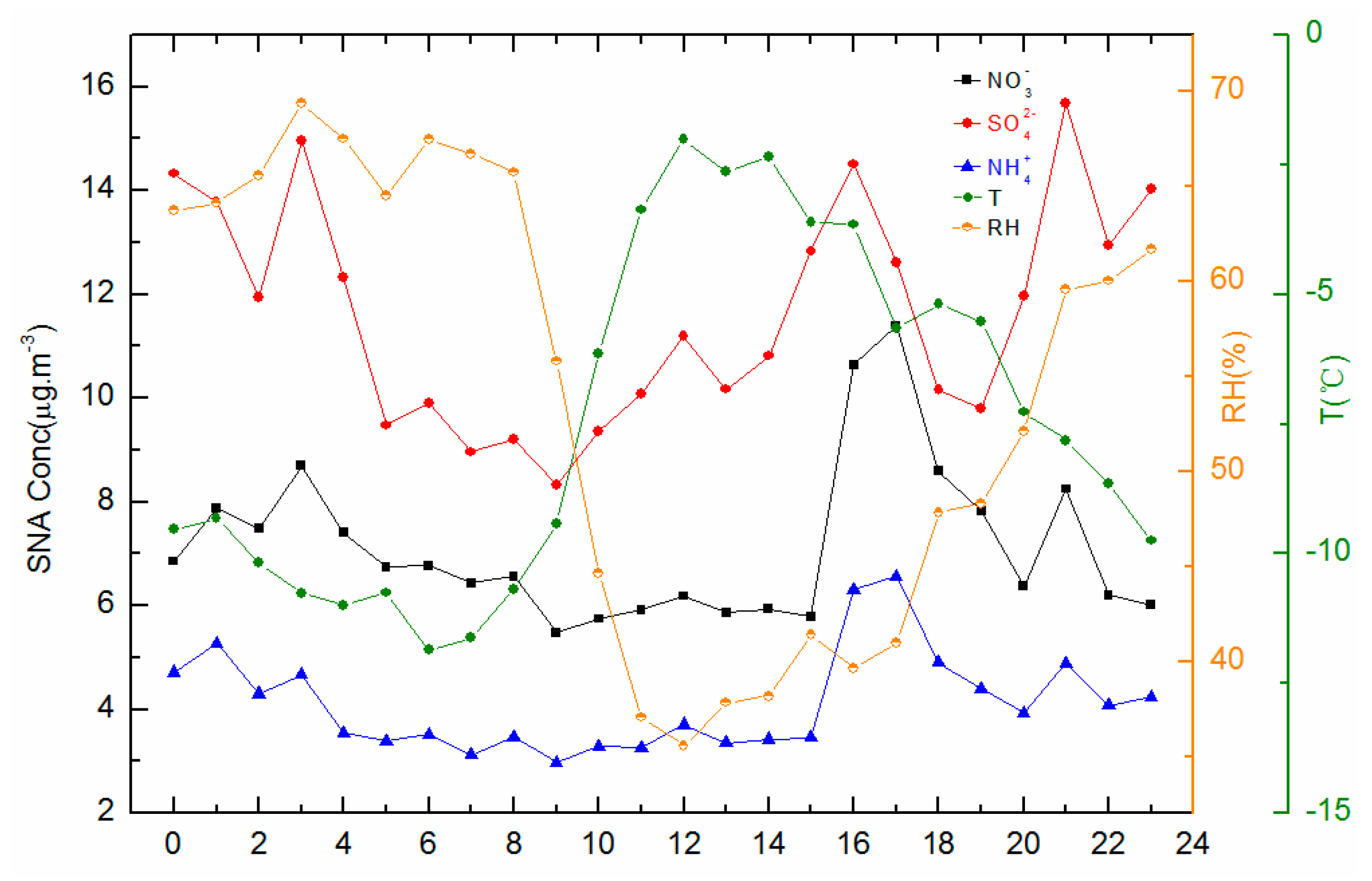
3.5. Diurnal Variations: Characteristic Differences between Haze and Non-Haze Days

Diurnal variations in all ions on non-haze days throughout all observation periods were significant (Figure 7). Clear diurnal variations can be seen from the chart, with the daily peaks of SO₄²⁻, NO₃⁻, and NH₄⁺ appearing at very similar times, indicating similar sources. Daily variations showed a pattern of three highs and two lows. The high peaks appeared at 00:00–03:00, 16:00–17:00 and 21:00, in line with the times when coal-burning heat was supplied in Shenyang. The period 16:00–17:00 also included the peak value of automobile exhaust emissions during commuting time. Anthropogenic activities normally peak after 08:00, yet the concentrations of pollutants did not increase during this period. The reason for this pattern may be that as the temperature rises after sunrise pollutants are rapidly diffused, the inversion layer weakens and the atmospheric boundary layer rises. The daily variation in SNA was similar to the changes in relative humidity and differed from the changes in temperature. The SNA concentrations on days with complex pollution exhibited obvious changes (Figure 8). In contrast to the non-haze periods, on complex-pollution days the correlations between SNA concentrations and temperature were higher than the correlations with relative humidity. Using Episode 2 in 2014 as an example, from 20:00 on 24 February to 09:00 on 25 February, relative humidity values were as high as 82–96%, while SO₄²⁻ and NH₄⁺ concentrations exhibited moderate increases but NO₃⁻ concentrations fell. During this period, concentrations of both NH₃ and O₃ were reduced. In addition, the height of the boundary layer remained constant at about 1.2 km and pressure conditions and sea-level pressure values remained virtually unchanged. A stable boundary layer, stable surface winds, and stable pressure fields minimize the likelihood of diffuse air flow to upper or adjacent areas of the atmosphere. Therefore, reduced NH₃ concentrations were likely the direct cause of the drop in NO₃⁻. Considering that relative humidity remained high beforehand, increasing NH₃ reacted with nitric and sulfuric acids. Specifically, when NH₃ was still abundant, it reacted quickly with nitric acid, leading to a constant rise in NO₃⁻ concentrations [12]. Once the NH₃ had been completely consumed, the precursor HNO₃ was still abundant, regardless of any further increase in humidity. However, NH₃ reacts with sulfuric acid faster than with nitric acid. In addition to the temperature drop, this hindered the reaction of NH₃ and nitric acid; consequently, NO₃⁻ concentrations decreased. Therefore, controls over NH₃ emissions should be a priority in the regulation of haze pollution in Shenyang.

4. Conclusions

Our results are summarized below.

(1) The average mass concentrations of PM_2.5 and TWSIs in PM₁₀ (PM_2.5) during haze episodes were 131 μg·m⁻³ and 77.2 μg·m⁻³, 2.3 times and 1.9 times the values in non-haze periods, respectively. The average mass concentration of TWSIs in PM_2.5 was 55.9 μg·m⁻³ (accounting for 55.9% of PM_2.5 mass loading), 37.6% of which was sulfate, 31.7% nitrate, 20.0% ammonium, 6.6% chloride, 1.9% potassium, 1.4% calcium, and 0.8% magnesium throughout the campaign. Concentrations of sulfate, nitrate, and ammonium (SNA) secondary pollution ions increased rapidly during haze episodes to as much as 2.2 times, 3.0 times, and 2.4 times higher than during non-haze periods, respectively. Concentrations of the natural ions Mg²⁺ and Ca²⁺ were also higher in non-haze periods than during hazy episodes.

In Shenyang, WS ions in PM₁₀ exhibited a state of neutrality.

(2) Based on changes in the backward trajectories and concentrations of WS ions, the hazy episodes were divided into three types: complex, coal-burning, and automobile exhaust pollution. All complex episodes had high concentrations, concentration of nitrate higher than that of sulfate, ranged from 32.3 μg·m⁻³ to 56 μg·m⁻³, with the percentage of TWSIs ranging from 33.3% to 43.6%. The NO₃⁻ percentage of TWSIs in automobile exhaust pollution ranged from 41.9% and 44.9%. Coal-burning was the most common source of pollution during winter in Shenyang. Contributions were higher from sulfate than from nitrate. This is also a common feature of winter pollution in Shenyang. SO₄²⁻ concentrations ranged from 13.4 μg·m⁻³ to 52.0 μg·m⁻³.

(3) Diurnal variations during non-haze periods were significant, while complex pollution was insignificant. Daily variations showed a pattern of three highs and two lows. The high peaks appeared at 00:00–03:00, 16:00–17:00, and 21:00.

(4) Summary of the Patterns of Presence and Sources of Three Categories of Pollution:

Complex-pollution episodes: SNA components were highly correlated, with nitrate and sulfate as the main forms, as is the case for automobile exhaust pollution. The correlation between K⁺ and Cl⁻ is very strong, and these ions exist mainly in the form KCl. Based on the results of PCA, the factor loads of SO₄²⁻, NO₃⁻, and NH₄⁺ were very high and were related to emissions from coal burning for heating and long-range transmission of pollution in winter. The high loads of Cl⁻ and Mg²⁺ were both related to local coal emissions and the desulfurization process. Several main factors combined to explain 70.2–89.0% of the total variance in contribution rates.

The PCA results for coal-burning episodes show that SO₄²⁻, NH₄⁺, and SO₂ had the highest factor loadings, and the contribution of coal-burning emissions was from 36.7% to 53.6%. Emissions were also related to industrial and soil sources and incomplete combustion by internal combustion engines.

In the case of automobile exhaust pollution, NH₄⁺ was more closely related to NO₃⁻ than to SO₄²⁻. The PCA results for automobile exhaust pollution were quite similar to those for complex pollution.

References

1. Yang, T.; Yan, P.Z.; Wang, Z.F.; Li, J.J.; Zhang, W.D.; Yao, X.F.; Wang, W.; Zhu, L.L.; Wu, H.Z. Evaluation and formation mechanism of a severe air pollution in Northeast China in November 2015. Acta Sci. Circumst. 2017, 37, 44–51. (In Chinese) [Google Scholar]
2. Xu, H.; Chen, J.Q.; He, D.T.; Cheng, P.; Wang, W.; Zhu, L.; Yao, H.; Gu, Z.Q. Climatic characteristics of haze weather during heating periods from 1980 to 2015 at Shenyang region. J. Meteorol. Environ. 2017, 33, 87–94. (In Chinese) [Google Scholar]
3. Wang, K.; Jia, L.L.; Huang, L.K.; Chui, C.; Wang, F.Y.; Lv, N.; Zhao, Q.L. Pollution characteristics of water-soluble ions in PM2.5 and PM10 under severe haze days. J. Harebin Inst. Technol. 2014, 46, 53–58. (In Chinese) [Google Scholar]
4. Jung, J.; Lee, H.; Kim, Y.J.; Liu, X.; Zhang, Y.; Gu, J.; Fan, S. Aerosol chemistry and the effect of aerosol water content on visibility impairment and radiative forcing in Guangzhou during the 2006 Pearl River Delta campaign. J. Environ. Manag. 2009, 90, 3231–3244. [Google Scholar] [CrossRef] [PubMed]
5. Fridlind, A.M.; Jacobson, M.Z. A study of gas-aerosol equilibrium and aerosol pH in the remote marine boundary layer during the First Aerosol Characterization Experiment (ACE 1). J. Geophys. Res. Atmos. 2000, 105, 17325–17340. [Google Scholar] [CrossRef] [Green Version]
6. Sun, Y.L.; Wang, Z.F.; Du, W.; Zhang, Q.; Wang, Q.Q.; Fu, P.Q.; Pan, X.L.; Li, J.; Jayne, J.; Worsnop, D.R. Long-term real-time measurements of aerosol particle composition in Beijing, China: Seasonal variations, meteorological effects, and source analysis. Atmos. Chem. Phys. 2015, 15, 10149–10165. [Google Scholar] [CrossRef]
7. Sun, Y.; Wang, Z.; Fu, P.; Jiang, Q.; Yang, T.; Li, J.; Ge, X. The impact of relative humidity on aerosol composition and evolution processes during wintertime in Beijing, China. Atmos. Environ. 2013, 77, 927–934. [Google Scholar] [CrossRef]
8. Kang, C.M.; Lee, H.S.; Kang, B.-W.; Lee, S.-K.; Sunwoo, Y. Chemical characteristics of acidic gas pollutants and PM2.5 species during hazy episodes in Seoul, South Korea. Atmos. Environ. 2004, 38, 4749–4760. [Google Scholar] [CrossRef]
9. Huang, Z.; Harrison, R.M.; Allen, A.G.; James, J.D.; Tilling, R.M.; Yin, J. Field intercomparison of filter pack and impactor sampling for aerosol nitrate, ammonium, and sulphate at coastal and inland sites. Atmos. Res. 2004, 71, 215–232. [Google Scholar] [CrossRef]
10. Hidy, G.M.; Appel, B.R.; Charlson, R.J.; Clark, W.E.; Friedlander, S.K.; Hutchison, D.H.; Smith, T.B.; Suder, J.; Wesolowski, J.J.; Whitby, K.T. summary of the California aerosol characterization experiment. J. Air Pollut. Control Assoc. 2012, 25, 1106–1114. [Google Scholar] [CrossRef]
11. Ottly, C.J.; Harrison, R.M. The spatial distribution and particle size of some inorganic nitrogen species over the North Sea. Atmos. Environ. 1992, 26, 1689–1699. [Google Scholar] [CrossRef]
12. Poulain, L.; Spindler, G.; Birmili, W.; Plass-Dülmer, C.; Wiedensohler, A.; Herrmann, H. Seasonal and diurnal variations of particulate nitrate and organic matter at the IfT research station Melpitz. Atmos. Chem. Phys. 2011, 11, 12579–12599. [Google Scholar] [CrossRef]
13. Petit, J.E.; Favez, O.; Sciare, J.; Crenn, V.; Sarda-Estève, R.; Bonnaire, N.; Močnik, G.; Dupont, J.C.; Haeffelin, M.; Leoz-Garziandia, E. Two years of near real-time chemical composition of submicron aerosols in the region of Paris using an Aerosol Chemical Speciation Monitor (ACSM) and a multi-wavelength Aethalometer. Atmos. Chem. Phys. 2015, 15, 2985–3005. [Google Scholar] [CrossRef]
14. Twigg, M.M.; Di Marco, C.F.; Leeson, S.; van Dijk, N.; Jones, M.R.; Leith, I.D.; Morrison, E.; Coyle, M.; Proost, R.; Peeters, A.N.M.; et al. Water soluble aerosols and gases at a UK background site—Part 1: Controls of PM2.5 and PM10 aerosol composition. Atmos. Chem. Phys. 2015, 15, 8131–8145. [Google Scholar] [CrossRef] [Green Version]
15. Mensah, A.A.; Holzinger, R.; Otjes, R.; Trimborn, A.; Mentel, T.F.; Ten Brink, H.; Henzing, B.; Kiendler-Scharr, A. Aerosol chemical composition at Cabauw, The Netherlands as observed in two intensive periods in May 2008 and March 2009. Atmos. Chem. Phys. 2012, 12, 4723–4742. [Google Scholar] [CrossRef] [Green Version]
16. Zhao, Y.N.; Wang, Y.S.; Wen, T.X.; Liu, Q. Characterization of water-soluble ions in PM2.5 at Dinghu Mount. Environ. Sci. 2013, 34, 1232–1235. (In Chinese) [Google Scholar]
17. Duan, F.; Liu, X.; Yu, T.; Cachier, H. Identification and estimate of biomass burning contribution to the urban aerosol organic carbon concentrations in Beijing. Atmos. Environ. 2004, 38, 1275–1282. [Google Scholar] [CrossRef]
18. Du, H.; Kong, L.; Cheng, T.; Chen, J.; Du, J.; Li, L.; Xia, X.; Leng, C.; Huang, G. Insights into summertime haze pollution events over Shanghai based on online water-soluble ionic composition of aerosols. Atmos. Environ. 2011, 45, 5131–5137. [Google Scholar] [CrossRef]
19. Pathak, R.K.; Wu, W.S.; Wang, T. Summertime PM2.5 ionic species in four major cities of China: Nitrate formation in an ammonia-deficient atmosphere. Atmos. Chem. Phys. 2009, 9, 1711–1722. [Google Scholar] [CrossRef] [Green Version]
20. Jongejan, P.A.C.; Bai, Y.; Veltkamp, A.C.; Wyers, G.P.; Slanina, J. An automated field instrument for the determination of acidic gases in air. Int. J. Environ. Anal. Chem. 1997, 66, 241–251. [Google Scholar] [CrossRef]
21. Khlystov, A.; Wyers, G.P.; Slanina, J. The steam-jet aerosol collector. Atmos. Environ. 1995, 29, 2229–2234. [Google Scholar] [CrossRef] [Green Version]
22. Trebs, I.; Meixner, F.X.; Slanma, J.; Otjes, R.; Jongejan, P.; Andreae, M.O. Realtime measurements of ammonia, acid trace gases and water-soluble inorganic aerosol species at a rural site in the Amazon Basin. Atmos. Chem. Phys. 2004, 4, 967–987. [Google Scholar] [CrossRef]
23. Li, L.; Huang, Z.; Dong, J.; Li, M.; Gao, W.; Nian, H.; Fu, Z.; Zhang, G.; Bi, X.; Cheng, P.; et al. Real time bipolar time-of-flight mass spectrometer for analyzing single aerosol particles. Int. J. Mass Spectrom. 2011, 303, 118–124. [Google Scholar] [CrossRef]
24. Song, C.H.; Carmichael, G.R. The aging process of naturally emitted aerosol (sea-salt and mineral aerosol) during long range transport. Atmos. Environ. 1999, 33, 2203–2218. [Google Scholar] [CrossRef]
25. Hopke, P.K.; Song, X.H. Classification of single particles by neural networks based on the computer-controlled scanning electron microscopy data. Anal. Chim. Acta 1997, 348, 375–388. [Google Scholar] [CrossRef]
26. Determination of Atmospheric Articles PM10 and PM2.5 in Ambient Air by Gravimetric Method. Available online: http://kjs.mep.gov.cn/hjbhbz/bzwb/jcffbz/201109/t20110914_217272.shtml. (accessed on 11 July 2018).
27. Technical Guidelines for Atmospheric Particulate Source Apportionment Proposed; Ministry of Environmental Protection of the People’s Republic of China: Beijing, China, 2013.
28. Observation and Forecast Level of Haze. In Standard of Meteorological Industry of the People’s Republic of China QX/T 113-2010; China Meteorological Administration: Beijing, China, 2010.
29. Sharma, S.K.; Mandal, T.K.; Srivastava, M.K.; Chatterjee, A.; Jain, S.; Saxena, M.; Singh, B.P.; Saraswati, A.; Sharma, A.; Adak, A.; et al. Spatio-temporal variation in chemical characteristics of PM10 over Indo Gangetic Plain of India. Environ. Sci. Pollut. Res. 2016, 23, 18809–18822. [Google Scholar] [CrossRef] [PubMed]
30. Lonati, G.; Giugliano, M.; Ozgen, S. Primary and Secondary Components of PM2.5 in Milan (Italy). Environ. Int. 2008, 34, 665–670. [Google Scholar] [CrossRef] [PubMed]
31. Qin, Y.; Kim, E.; Hopke, P.K. The Concentrations and Sources of PM2.5 in Metropolitan New York City. Atmos. Environ. 2006, 40, S312–S332. [Google Scholar] [CrossRef]
32. Biswas, K.; Badar, F.; Ghauri, M.; Husain, L. Gaseous and Aerosol Pollutants during Fog and Clear Episodes in South Asian Urban Atmosphere. Atmos. Environ. 2008, 42, 7775–7785. [Google Scholar] [CrossRef]
33. Yao, Y.G.; Zou, Q.; Chen, C.; Zhang, X.H.; Liu, H.J.; Kang, X.F. The Analysis of chemical component of PM2.5 on haze formation in Suzhou City. Environ. Monit. China 2014, 30, 62–68. (In Chinese) [Google Scholar]
34. Zhou, Y.Y.; Ma, Y.; Zheng, J.; Cui, F.P.; Wang, L. Pollution characteristics and light extinction effects of water-soluble Ions in PM2.5 during winter hazy days at north suburban Nanjing. Environ. Sci. 2015, 36, 1926–1934. (In Chinese) [Google Scholar]
35. Kong, S.F.; Li, L.; Li, X.X.; Yin, Y.; Chen, K.; Liu, D.T.; Ji, Y.Q. The impacts of firework burning at the Chinese Spring Festival on air quality: Insights of tracers, source evolution and aging processes. Atmos. Chem. Phys. 2015, 15, 2167–2184. (In Chinese) [Google Scholar] [CrossRef]
36. Liu, J.; Wu, D.; Fan, S.J.; Wu, M. Pollution characteristics during haze and clean processes in Guangzhou. Acta Sci. Circumst. 2015, 35, 3433–3442. (In Chinese) [Google Scholar]
37. Wang, H.B.; Tian, M.; Li, X.; Chang, Q.; Cao, J.; Yang, F.; Ma, Y.L.; He, K.B. Chemical composition and light extinction contribution of PM2.5 in urban Beijing for a 1-year period. Aerosol Air Qual. Res. 2015, 15, 2200–2211. [Google Scholar] [CrossRef]
38. Shen, J.C.; Chen, C.; Duo, K.X. Pollution characteristics of water soluble Ions in PM2.5 in some cities of central China. Environ. Sci. Technol. 2014, 37, 153–156. [Google Scholar]
39. Fang, J.L.; Liu, Z.; Wang, H.W.; Hao, S.X.; Dong, X.Y. Distribution characteristics and influencing factors of nine water-soluble ions in PM2.5 in Beijing. J. Environ. Health 2016, 33, 317–319. (In Chinese) [Google Scholar]
40. Chen, N.; Quan, J.H.; Tian, Y.P.; Cao, W.X.; Liu, H.; Zheng, M.M.; Liu, L.; Hu, H. The Physical and Chemical Properties of Atmospheric Pollutant in Wuhan Urban Area during the Haze. Environ. Monit. China 2016, 32, 20–25. (In Chinese) [Google Scholar]
41. Yao, C.T. Changes of Chemical Compositions of Atmospheric Fine Particles during a Typical Haze Event in Taiyuan. Master’s Thesis, Shanxi University, Taiyuan, China, 1 June 2013. (In Chinese). [Google Scholar]
42. Sun, J.; Zhang, Q.; Canagaratna, M.R.; Zhang, Y.; Ng, N.L.; Sun, Y.; Jayne, J.T.; Zhang, X.; Zhang, X.; Worsnop, D.R. Highly time- and size-resolved characterization of submicron aerosol particles in Beijing using an Aerodyne Aerosol Mass Spectrometer. Atmos. Environ. 2010, 44, 131–140. [Google Scholar] [CrossRef]
43. Liu, J.; Zhang, X.L.; Xu, X.F.; Xu, H.H. Comparison analysis of variation characteristics of SO2, NOx, O3 and PM2.5 between rural and urban areas, Beijing. Environ. Sci. 2008, 29, 1059–1065. (In Chinese) [Google Scholar]
44. McLaren, R.; Salmon, R.A.; Liggio, J.; Hayden, K.L.; Anlauf, K.G.; Leaitch, W.R. Nighttime chemistry at a rural site in the Lower Fraser Valley. Atmos. Environ. 2004, 38, 5837–5848. [Google Scholar] [CrossRef] [Green Version]
45. Zhang, Y.J.; Tang, L.L.; Wang, Z.; Yu, H.X.; Sun, Y.L.; Liu, D.; Qin, W.; Canonaco, F.; Prévôt, A.S.H.; Zhang, H.L.; et al. Insights into characteristics, sources, and evolution of submicron aerosols during harvest seasons in the Yangtze River delta region, China. Atmos. Chem. Phys. 2015, 15, 1331–1349. [Google Scholar] [CrossRef]
46. Hu, W.W.; Hu, M.; Yuan, B.; Jimenez, J.L.; Tang, Q.; Peng, J.F.; Hu, W.; Shao, M.; Wang, M.; Zeng, L.M.; et al. Insights on organic aerosol aging and the influence of coal combustion at a regional receptor site of central eastern China. Atmos. Chem. Phys. 2013, 13, 10095–10112. [Google Scholar] [CrossRef] [Green Version]
47. Wang, X.Q.; Yang, T.; Wang, Z.F. Impact of dust-haze episode from one air pollution control region to the other-one caxe study. Clim. Environ. Res. 2011, 16, 690–696. (In Chinese) [Google Scholar]
48. Hong, Y.; Ma, Y.J.; Wang, X.Q.; Zhang, Y.H.; Lu, Z.Y.; Wang, Y.F.; Zhou, D.P.; Liu, N.W. External influences in the haze episode in the central city group of Liaoning: A case study. Acta Sci. Circumst. 2013, 33, 2115–2122. (In Chinese) [Google Scholar]
49. Yang, T.; Wang, X.Q.; Wang, Z.F. Gravity current driven transport of haze from North China Plain to North east China in Winter 2010 Part 2: Model simulation with tagged tracers. SOLA 2013, 9, 60–64. [Google Scholar] [CrossRef]
50. Sun, Y.L.; Wang, Z.F.; Fu, P.Q.; Yang, T.; Jiang, Q.; Dong, H.B.; Li, J.; Jia, J.J. Aerosol composition, sources and processes during wintertime in Beijing, China. Atmos. Chem. Phys. 2013, 13, 4577–4592. [Google Scholar] [CrossRef]
51. Chow, J.C. Measurement methods to determine compliance with ambient air quality standards for suspended particles. J. Air Waste Manag. Assoc. 1995, 45, 320–382. [Google Scholar] [CrossRef] [PubMed]
52. Xu, W.Y.; Zhao, C.S.; Ran, L.; Lin, W.L.; Yan, P.; Xu, X.B. SO2 noontime-peak phenomenon in the North China Plain. Atmos. Chem. Phys. 2014, 14, 7757–7768. [Google Scholar] [CrossRef]
53. Farnham, I.M.; Johannesson, K.H.; Singh, A.K. Factor analytical approaches for evaluating groundwater trace element chemistry data. Anal. Chim. Acta 2003, 490, 123–138. [Google Scholar] [CrossRef]
54. He, P.; Li, S.S.; Zhu, W.Q.; Sun, Z.Q.; Liang, W. How wet desulfurization cause large area Smog. Sci. Manag. 2017, 37, 7–11. (In Chinese) [Google Scholar]
55. Zhu, T.; Shang, J.; Zhao, D. The roles of heterogeneous chemical processes in the formation of an air pollution complex and gray haze. Sci. China 2010, 40, 1731–1740. [Google Scholar] [CrossRef]
56. Brown, S.S.; Stark, H.; Ryerson, T.B.; Williams, E.J.; Nicks, D.K.; Trainer, M.; Fehsenfeld, F.C.; Ravishankara, A.R. Nitrogen oxides in the nocturnal boundary layer, Simultaneous in situ measurements of NO3, N2O5, NO2, NO, and O3. J. Geophys. Res. Atmos. 2003, 108, 4299. [Google Scholar] [CrossRef]
57. Wang, Y.; Zhuang, G.; Sun, Y.; An, Z. The variation of characteristics and formation mechanisms of aerosols in dust, haze, and clear days in Beijing. Atmos. Environ. 2006, 40, 6579–6591. [Google Scholar] [CrossRef]
58. Zhang, N.N.; He, Y.Q.; Wang, C.F.; He, X.Z.; Xin, H.J. Chemical characteristic of water-soluble ions in total suspended particles (TSP) at Lijiang winter time. Atmos. Environ. 2011, 32, 619–625. [Google Scholar]
59. Chen, Y.Q.; Zhang, Y.; Wang, Z.W.; Zhang, X.S. Property of Water-soluble ion of aerosol particle in different area in Beijing. Environ. Chem. 2004, 23, 674–680. [Google Scholar]
60. Tan, J.H.; Duan, J.C.; Chen, D.H.; Wang, X.H.; Guo, S.J.; Bi, X.H.; Sheng, G.Y.; He, K.B.; Fu, J.M. Chemical characteristics of haze during summer and winter in Guangzhou. Atmos. Res. 2009, 94, 238–245. [Google Scholar] [CrossRef]
Figure 1. Schematic map of the sampling location (a) and a Terra satellite true color image of northeastern China, taken on 25 February 2014 (b).
Atmosphere 09 00280 g001
Figure 2. Time series PM10 sources during the study periods in 2014. Hatched frames refer to the identified haze pollution episodes.
Atmosphere 09 00280 g002
Figure 3. Time series of hourly concentrations (μg·m−3) of TWSIs (include SO42−, NO3, NH4+, Cl, K+, Mg2+, and Ca2+) of PM10, PM2.5, gaseous SO2 and NO2, atmospheric visibility (Vis, km), relative humidity (RH, %), pressure (P, hpa), temperature (T, °C), wind direction (WD, °), and wind speed (WS, m·s−1), measured over the ambient observation period. Hatched frames refer to the identified haze pollution episodes.
Atmosphere 09 00280 g003
Figure 4. Comparison of measured and calculated NH4+ mass concentrations (the red line represents slope, R2).
Atmosphere 09 00280 g004
Figure 5. Mean 72-h backward trajectories of pollutions Episodes 1–9 (red, blue, and green lines represent air masses 500, 1000, and 2000 m above sea level, respectively).
Atmosphere 09 00280 g005
Figure 6. The pie charts show the concentrations (µg·m−3) and mass fractions (%) of each aerosol species in TWSIs during pollution Episodes 1–9 and the entire study period (upper part of the figure shows the concentrations of PM10 and PM2.5 during these episodes in parentheses).
Atmosphere 09 00280 g006
Figure 7. Diurnal variations in SO42−, NO3, and NH4+ (SNA), relative humidity (RH, %), and temperature (T, °C) on non-haze days.
Atmosphere 09 00280 g007
Figure 8. Diurnal variations in SO42−, NO3, and NH4+ (SNA), relative humidity (RH, %), and temperature (T, °C) on days influenced by complex pollution.
Atmosphere 09 00280 g008