Potential of Sentinel-1 Images for Estimating the Soil Roughness over Bare Agricultural Soils

 , , ,
, , ,
Abstract
:1. Introduction
2. Methods and Materials
2.1. Methodological Overview
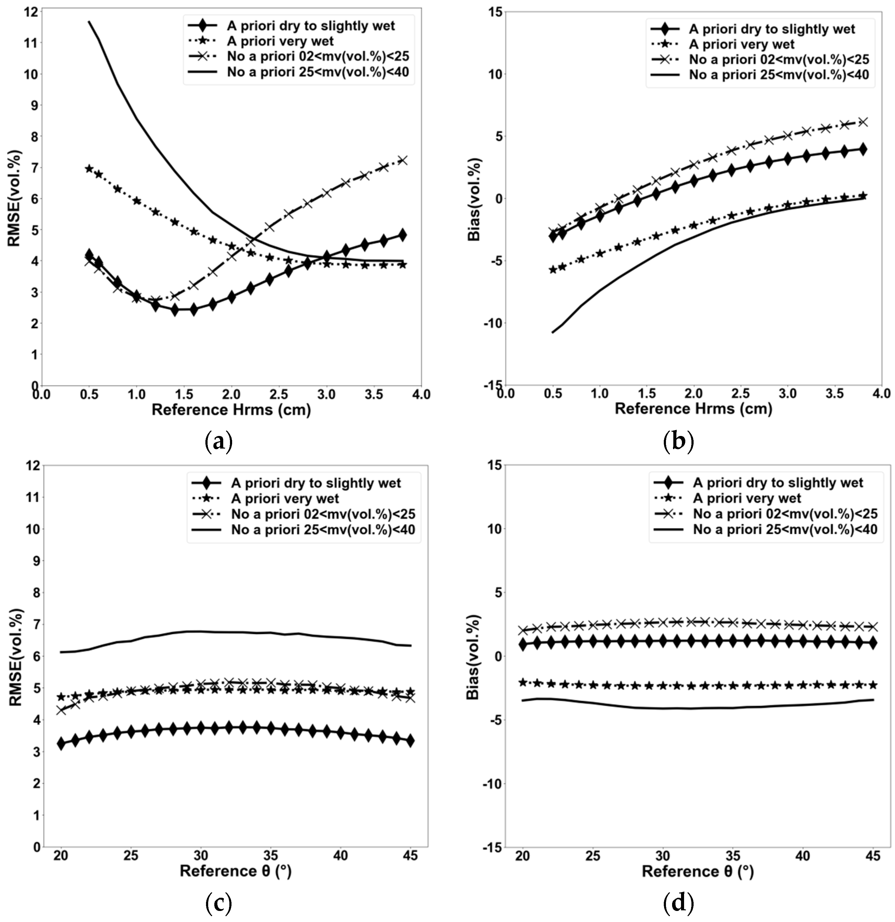
- Case 1: No a priori information is available on the soil moisture status. In this case mv is estimated between 2 and 40 vol. %.
- Case 2: A priori information is available on mv. The soil is supposed to be dry to slightly wet according to expertise based mainly on meteorological data (precipitations, temperature). Soil moisture values are assumed to range from 2 to 25 vol. %.
- Case 3: A priori information is available on mv. The soil is supposed to be very wet according to expertise based on meteorological data. mv-values are assumed to vary between 25 and 40 vol. %.
2.2. Artificial Neural Networks (Ann)
2.3. Dataset Description
2.3.1. Synthetic Dataset
2.3.2. Real Dataset
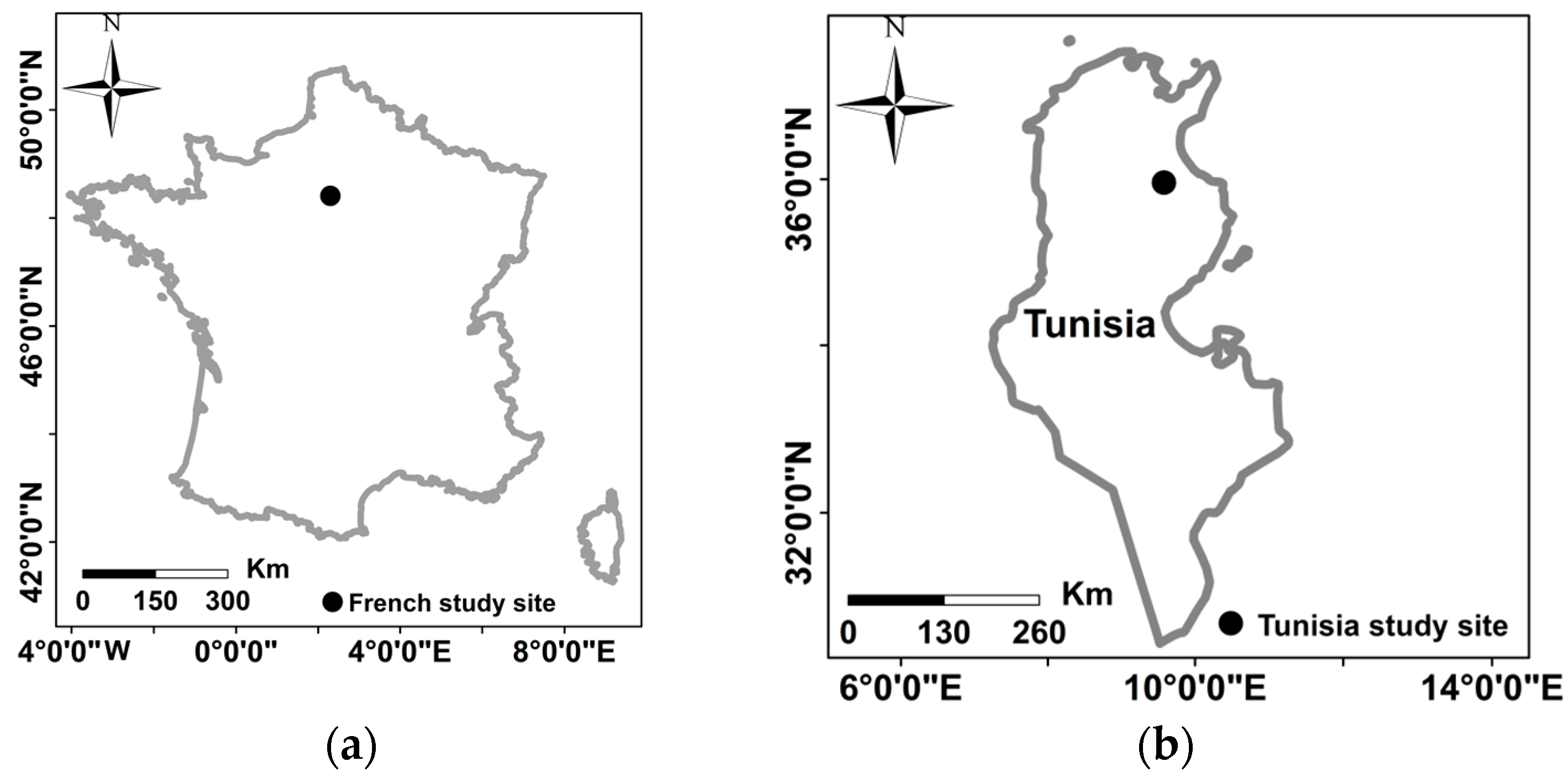
Study Sites
SAR Satellite Images
In Situ Measurements
3. Results and Discussion
3.1. Synthetic Dataset
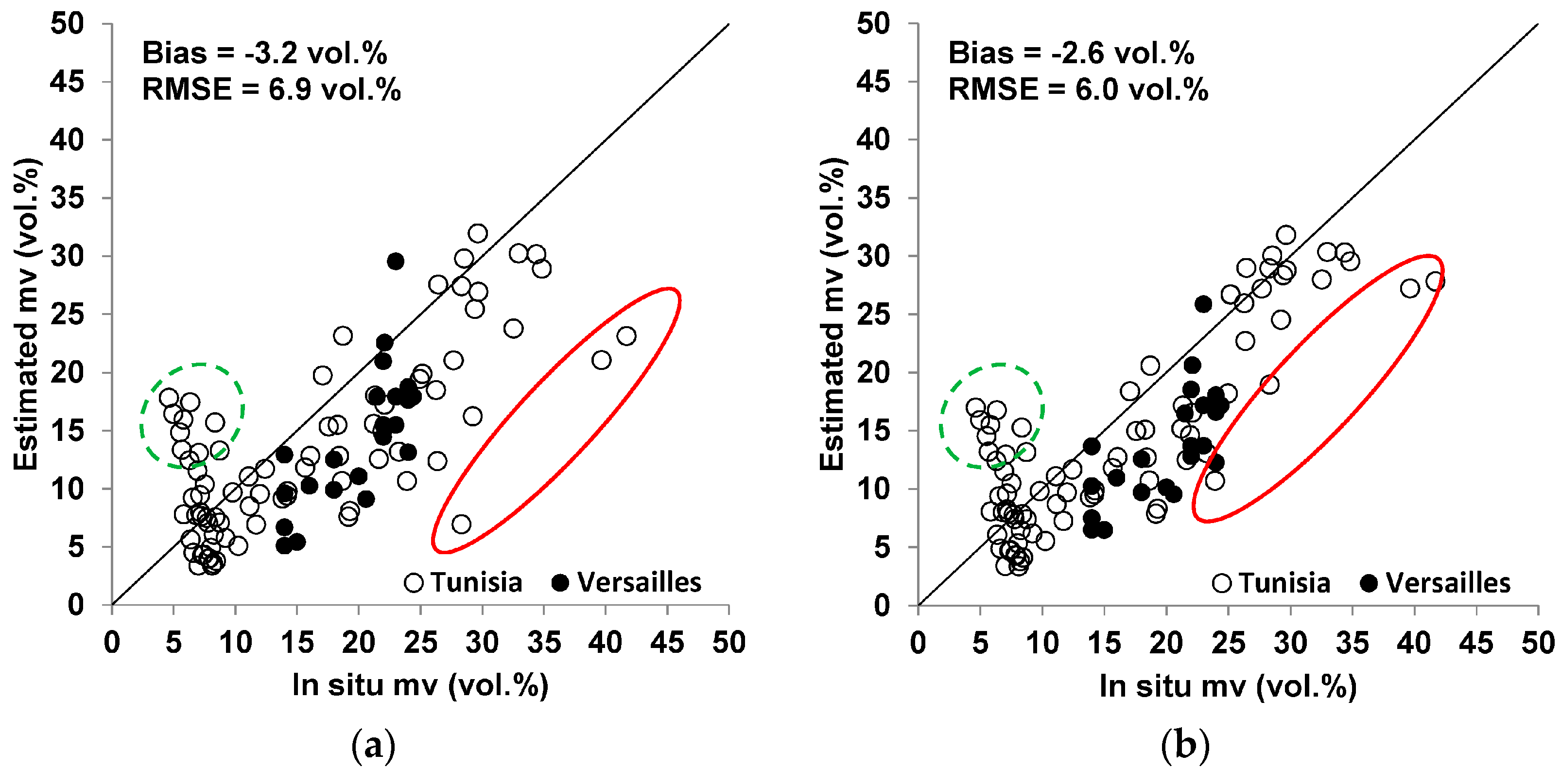
3.1.1. Estimation of mv
Case 1: No a Priori Information on the Soil Moisture State
Case 2: A Priori Information on mv: Dry to Slightly Wet Soils (2 to 25 vol. %)
Case 3: A Priori Information on mv: Very Wet Soils (25 to 40 vol. %)
Discussion
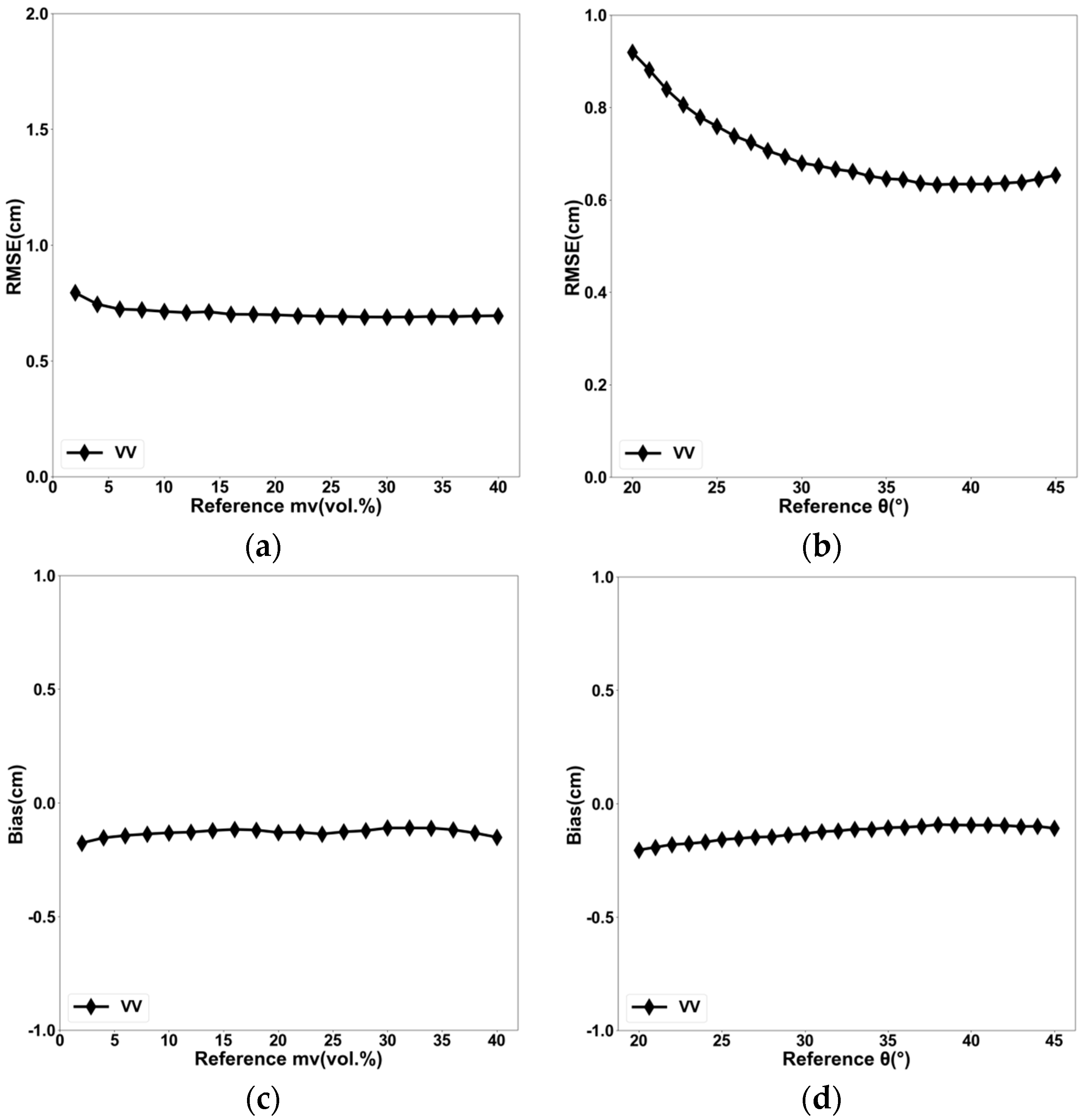
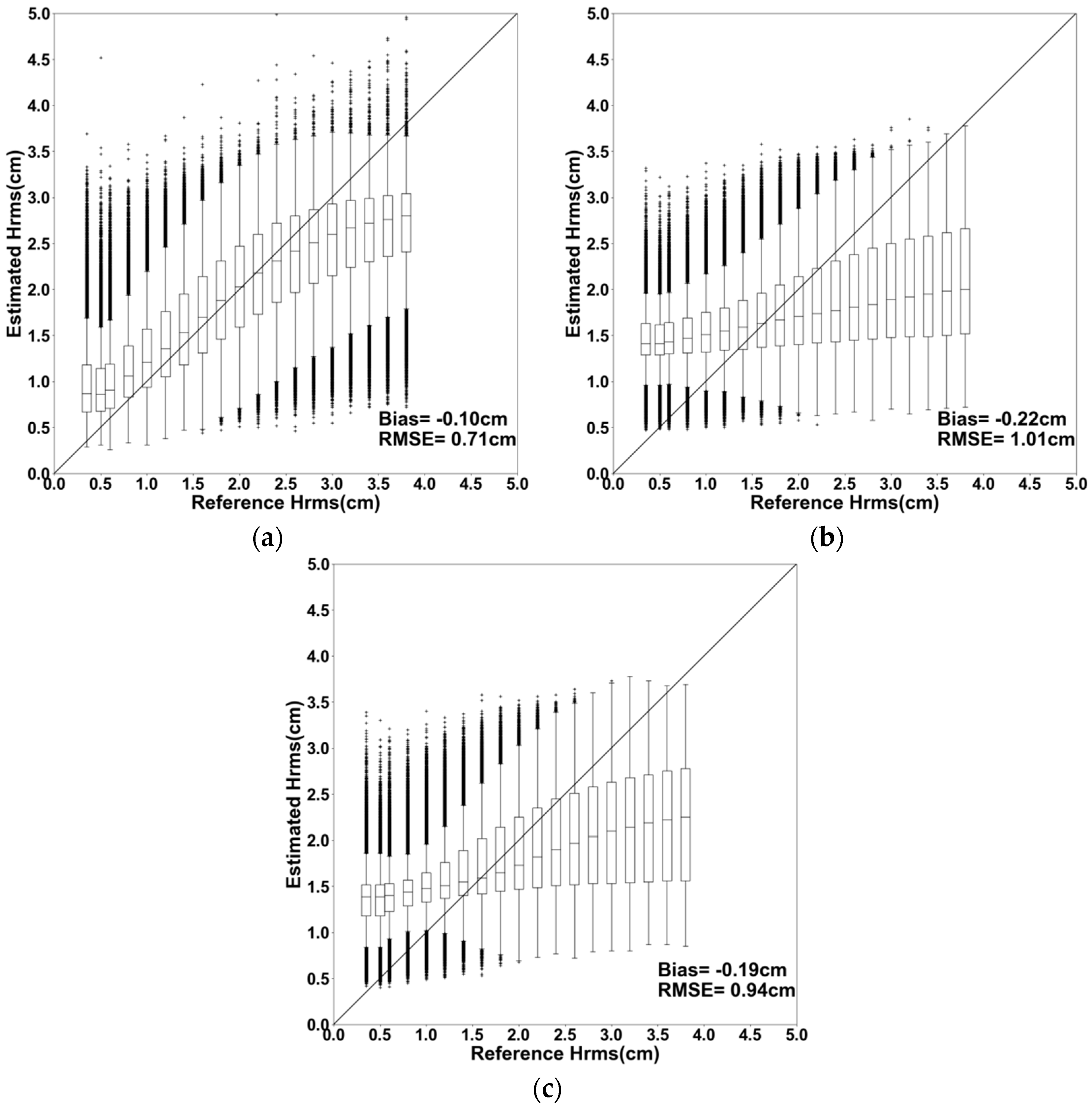
3.1.2. Estimation of Hrms
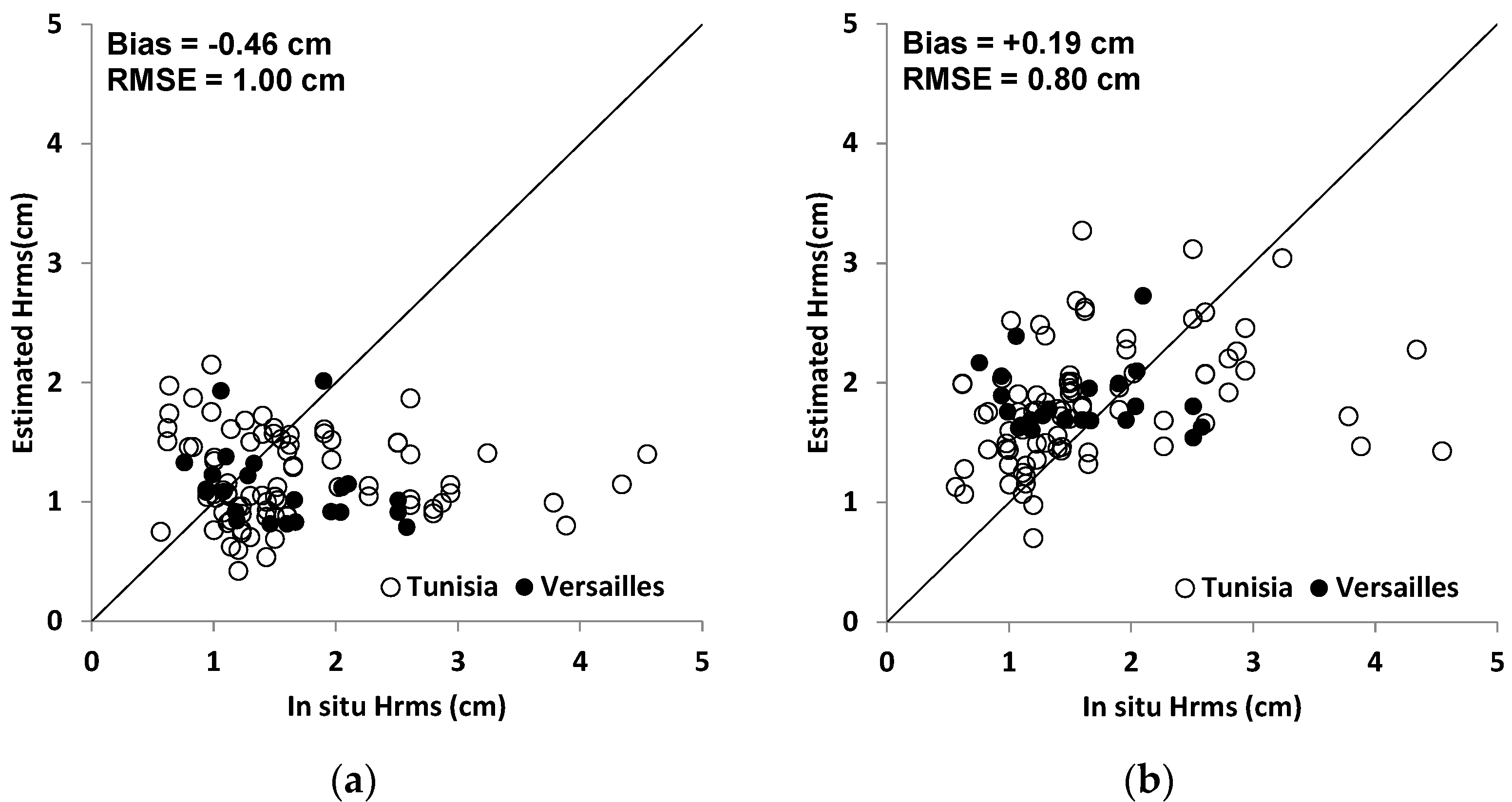
3.2. Real Dataset
- At the input of the network for the estimation of Hrms, the mv used corresponds to mv estimated at plot scale (using the mean radar signal calculated by averaging for each reference plot the values of all pixels within the reference plot).
- At the input of the network for the estimation of Hrms, the mv used corresponds to mv estimated at the scale of the study site (using the mean radar signal calculated by averaging the values of all bare soil pixels within the study site).
4. Conclusions
Acknowledgments
Author Contributions
Conflicts of Interest
References
- Ogilvy, J.A.; Merklinger, H.M. Theory of wave scattering from random rough surfaces. J. Acoust. Soc. Am. 1991, 90, 3382. [Google Scholar] [CrossRef]
- Baghdadi, N.; Choker, M.; Zribi, M.; Hajj, M.E.; Paloscia, S.; Verhoest, N.E.; Lievens, H.; Baup, F.; Mattia, F. A new empirical model for radar scattering from bare soil surfaces. Remote Sens. 2016, 8, 920. [Google Scholar] [CrossRef]
- Zribi, M.; Gorrab, A.; Baghdadi, N. A new soil roughness parameter for the modelling of radar backscattering over bare soil. Remote Sens. Environ. 2014, 152, 62–73. [Google Scholar] [CrossRef] [Green Version]
- Aubert, M.; Baghdadi, N.; Zribi, M.; Douaoui, A.; Loumagne, C.; Baup, F.; El Hajj, M.; Garrigues, S. Analysis of TerraSAR-X data sensitivity to bare soil moisture, roughness, composition and soil crust. Remote Sens. Environ. 2011, 115, 1801–1810. [Google Scholar] [CrossRef] [Green Version]
- Baghdadi, N.; King, C.; Bourguignon, A.; Remond, A. Potential of ERS and RADARSAT data for surface roughness monitoring over bare agricultural fields: Application to catchments in Northern France. Int. J. Remote Sens. 2002, 23, 3427–3442. [Google Scholar] [CrossRef]
- Baghdadi, N.; Zribi, M.; Loumagne, C.; Ansart, P.; Anguela, T.P. Analysis of TerraSAR-X data and their sensitivity to soil surface parameters over bare agricultural fields. Remote Sens. Environ. 2008, 112, 4370–4379. [Google Scholar] [CrossRef]
- Baghdadi, N.; Cerdan, O.; Zribi, M.; Auzet, V.; Darboux, F.; El Hajj, M.; Kheir, R.B. Operational performance of current synthetic aperture radar sensors in mapping soil surface characteristics in agricultural environments: Application to hydrological and erosion modelling. Hydrol. Process. 2008, 22, 9–20. [Google Scholar] [CrossRef]
- Fung, A.K. Microwave Scattering and Emission Models and Their Applications; Artech House: Boston, MA, USA, 1994. [Google Scholar]
- Zribi, M.; Dechambre, M. A new empirical model to retrieve soil moisture and roughness from C-band radar data. Remote Sens. Environ. 2002, 84, 42–52. [Google Scholar] [CrossRef]
- Baghdadi, N.; Gaultier, S.; King, C. Retrieving surface roughness and soil moisture from SAR data using neural networks. In Retrieval of Bio- and Geo-Physical Parameters from SAR Data for Land Applications; ESTEC Publishing Division: Sheffield, UK, 2002; pp. 315–319. [Google Scholar]
- Ulaby, F.T.; Moore, R.K.; Fung, A.K. Microwave Remote Sensing: Active and Passive, Vol. III, Volume Scattering and Emission Theory, Advanced Systems and Applications; Artech House, Inc.: Dedham, MA, USA, 1986; pp. 1797–1848. [Google Scholar]
- Holah, N.; Baghdadi, N.; Zribi, M.; Bruand, A.; King, C. Potential of ASAR/ENVISAT for the characterization of soil surface parameters over bare agricultural fields. Remote Sens. Environ. 2005, 96, 78–86. [Google Scholar] [CrossRef] [Green Version]
- Aubert, M.; Baghdadi, N.N.; Zribi, M.; Ose, K.; El Hajj, M.; Vaudour, E.; Gonzalez-Sosa, E. Toward an Operational Bare Soil Moisture Mapping Using TerraSAR-X Data Acquired Over Agricultural Areas. IEEE J. Sel. Top. Appl. Earth Obs. Remote Sens. 2013, 6, 900–916. [Google Scholar] [CrossRef] [Green Version]
- Baghdadi, N.; Camus, P.; Beaugendre, N.; Issa, O.M.; Zribi, M.; Desprats, J.F.; Rajot, J.L.; Abdallah, C.; Sannier, C. Estimating surface soil moisture from TerraSAR-X data over two small catchments in the Sahelian Part of Western Niger. Remote Sens. 2011, 3, 1266–1283. [Google Scholar] [CrossRef] [Green Version]
- Baghdadi, N.; Cresson, R.; El Hajj, M.; Ludwig, R.; La Jeunesse, I. Estimation of soil parameters over bare agriculture areas from C-band polarimetric SAR data using neural networks. Hydrol. Earth Syst. Sci. 2012, 16, 1607–1621. [Google Scholar] [CrossRef] [Green Version]
- El Hajj, M.; Baghdadi, N.; Zribi, M.; Belaud, G.; Cheviron, B.; Courault, D.; Charron, F. Soil moisture retrieval over irrigated grassland using X-band SAR data. Remote Sens. Environ. 2016, 176, 202–218. [Google Scholar] [CrossRef]
- Paloscia, S.; Pettinato, S.; Santi, E.; Notarnicola, C.; Pasolli, L.; Reppucci, A. Soil moisture mapping using Sentinel-1 images: Algorithm and preliminary validation. Remote Sens. Environ. 2013, 134, 234–248. [Google Scholar] [CrossRef]
- Zribi, M.; Chahbi, A.; Shabou, M.; Lili-Chabaane, Z.; Duchemin, B.; Baghdadi, N.; Amri, R.; Chehbouni, A. Soil surface moisture estimation over a semi-arid region using ENVISAT ASAR radar data for soil evaporation evaluation. Hydrol. Earth Syst. Sci. 2011, 15, 345–358. [Google Scholar] [CrossRef] [Green Version]
- El Hajj, M.; Baghdadi, N.; Zribi, M.; Bazzi, H. Synergic use of Sentinel-1 and Sentinel-2 images for operational soil moisture mapping at high spatial resolution over agricultural areas. Remote Sens. 2017, 9, 1292. [Google Scholar] [CrossRef]
- Schwerdt, M.; Schmidt, K.; Tous Ramon, N.; Klenk, P.; Yague-Martinez, N.; Prats-Iraola, P.; Zink, M.; Geudtner, D. Independent System Calibration of Sentinel-1B. Remote Sens. 2017, 9, 511. [Google Scholar] [CrossRef]
- Marquardt, D.W. An algorithm for least-squares estimation of nonlinear parameters. J. Soc. Ind. Appl. Math. 1963, 11, 431–441. [Google Scholar] [CrossRef]
- Notarnicola, C.; Angiulli, M.; Posa, F. Soil moisture retrieval from remotely sensed data: Neural network approach versus Bayesian method. IEEE Trans. Geosci. Remote Sens. 2008, 46, 547–557. [Google Scholar] [CrossRef]
- Satalino, G.; Mattia, F.; Davidson, M.W.; Le Toan, T.; Pasquariello, G.; Borgeaud, M. On current limits of soil moisture retrieval from ERS-SAR data. IEEE Trans. Geosci. Remote Sens. 2002, 40, 2438–2447. [Google Scholar] [CrossRef]
- Baghdadi, N.; Holah, N.; Zribi, M. Calibration of the integral equation model for SAR data in C-band and HH and VV polarizations. Int. J. Remote Sens. 2006, 27, 805–816. [Google Scholar] [CrossRef]
- Baghdadi, N.; Chaaya, J.A.; Zribi, M. Semiempirical calibration of the integral equation model for SAR data in C-band and cross polarization using radar images and field measurements. IEEE Geosci. Remote Sens. Lett. 2011, 8, 14–18. [Google Scholar] [CrossRef]
- Baghdadi, N.; Zribi, M. Characterization of Soil Surface Properties Using Radar Remote Sensing. In Land Surface Remote Sensing in Continental Hydrology; Elsevier: Amsterdam, The Netherlands, 2016; pp. 1–39. [Google Scholar]
- Hallikainen, M.T.; Ulaby, F.T.; Dobson, M.C.; El-Rayes, M.A.; Wu, L.-K. Microwave dielectric behavior of wet soil-part 1: Empirical models and experimental observations. IEEE Trans. Geosci. Remote Sens. 1985, 23, 25–34. [Google Scholar] [CrossRef]
- Vaudour, E.; Baghdadi, N.; Gilliot, J.-M. Mapping tillage operations over a peri-urban region using combined SPOT4 and ASAR/ENVISAT images. Int. J. Appl. Earth Obs. Geoinform. 2014, 28, 43–59. [Google Scholar] [CrossRef]
- Gorrab, A.; Zribi, M.; Baghdadi, N.; Mougenot, B.; Chabaane, Z.L. Potential of X-Band TerraSAR-X and COSMO-SkyMed SAR Data for the Assessment of Physical Soil Parameters. Remote Sens. 2015, 7, 747–766. [Google Scholar] [CrossRef] [Green Version]
- Gilliot, J.-M.; Vaudour, E.; Michelin, J. Soil surface roughness measurement: A new fully automatic photogrammetric approach applied to agricultural bare fields. Comput. Electron. Agric. 2017, 134, 63–78. [Google Scholar] [CrossRef]
- Bousbih, S.; Zribi, M.; Lili-Chabaane, Z.; Baghdadi, N.; El Hajj, M.; Gao, Q.; Mougenot, B. Potential of Sentinel-1 Radar Data for the Assessment of Soil and Cereal Cover Parameters. Sensors 2017, 17, 2617. [Google Scholar] [CrossRef] [PubMed]


| Site | SAR Sensor | Incidence Angle (°) | Dates (Day/Month/Year) | Number of Data |
|---|---|---|---|---|
| French site | Sentinel-1 | ~37° | 15/3/2017; 27/3/2017 2/4/2017; 8/4/2017 | 24 measurements |
| Tunisian site | Sentinel-1 | ~39° to 41° | 18/12/2015; 4/2/2016 3/4/2016; 4/4/2016 23/12/2016; 5/1/2017 9/2/2017 | 85 measurements |
© 2018 by the authors. Licensee MDPI, Basel, Switzerland. This article is an open access article distributed under the terms and conditions of the Creative Commons Attribution (CC BY) license (http://creativecommons.org/licenses/by/4.0/).
Share and Cite
Baghdadi, N.; El Hajj, M.; Choker, M.; Zribi, M.; Bazzi, H.; Vaudour, E.; Gilliot, J.-M.; Ebengo, D.M. Potential of Sentinel-1 Images for Estimating the Soil Roughness over Bare Agricultural Soils. Water 2018, 10, 131. https://doi.org/10.3390/w10020131
Baghdadi N, El Hajj M, Choker M, Zribi M, Bazzi H, Vaudour E, Gilliot J-M, Ebengo DM. Potential of Sentinel-1 Images for Estimating the Soil Roughness over Bare Agricultural Soils. Water. 2018; 10(2):131. https://doi.org/10.3390/w10020131
Chicago/Turabian StyleBaghdadi, Nicolas, Mohammad El Hajj, Mohammad Choker, Mehrez Zribi, Hassan Bazzi, Emmanuelle Vaudour, Jean-Marc Gilliot, and Dav M. Ebengo. 2018. "Potential of Sentinel-1 Images for Estimating the Soil Roughness over Bare Agricultural Soils" Water 10, no. 2: 131. https://doi.org/10.3390/w10020131