Global Sensitivity Analysis of a Water Quality Model in the Three Gorges Reservoir


1
State Key Laboratory of Simulation and Regulation of Water Cycle in River Basin, China Institute of Water Resources and Hydropower Research, Beijing 100038, China
2
School of Water Conservancy and Hydroelectric Power, Hebei University of Engineering, Handan 056002, China
3
Key Laboratory of Marine Environment and Ecology, Ministry of Education, Ocean University of China, Qingdao 266100, China
*
Author to whom correspondence should be addressed.
Water 2018, 10(2), 153; https://doi.org/10.3390/w10020153
Submission received: 6 December 2017
/
Revised: 29 January 2018
/
Accepted: 31 January 2018
/
Published: 5 February 2018
Abstract
:Global sensitivity analysis is the key to establishing advanced and complex water quality models and measurements of ecological parameters. In this paper, the Sobol’s sensitivity analysis method was applied to a quantitative analysis of the important factors governing a water quality model, which has been developed to simulate algal dynamics in Caotang Bay, one of the tributary bays in the Three Gorges Reservoir, China. The analysis focused on the response of chlorophyll-a and dissolved oxygen to 11 parameters. The results show that chlorophyll-a is influenced mainly by the maximum phytoplankton growth rate, the lower optimum temperature for algal growth, the phosphate half-saturation constant, and the phytoplankton linear mortality rate; while dissolved oxygen is influenced mainly by the maximum phytoplankton growth rate, the lower optimum temperature for algal growth, the phytoplankton basal respiration rate, and the detritus remineralization rate. These parameter sensitivities change with time and have a marked seasonal pattern. The parameter sensitivity differences between a shallow lake or reservoir and a deep reservoir suggest that mechanisms of cycling in nutrients and dissolved oxygen are different.
1. Introduction
Water quality models are valuable tools for the quantitative analysis of a water system’s evolution processes [1,2,3]. Research on water quality models is aimed at exploring the varying mechanisms of the ecosystem, simulating or predicting its changes, and providing scientific and decision-making rationales in order to maintain its health and recover its injured parts. Parameters are an important component of the ecological model, ranging from ten to dozens of variables [4,5,6,7] depending on the complexity of the model. It is very difficult to increase the precision of each parameter at the same time, as surface water is a highly nonlinear system, so each ecological process will be subject to various uncertain factors.
The model is the mathematical expression of the ecological process, and Sensitivity Analysis (SA) aims to characterize the impact that changes in the model’s input factors (e.g., parameters, initial states, input data, time/spatial resolution grid) have on the model’s output (e.g., a statistic of the simulated time series, such as the average simulated stream flow, or an objective function, such as the Root Mean Squared Error). SA represents how the sensitive the modeled ecological process response is to the environmental condition input to the model. SA methods can be classified based on their scope, applicability, and characteristics. The simplest and most common classifications are local sensitivity analysis (LSA) and global sensitivity analysis (GSA) [8,9,10]. LSA is focused on the effects of uncertain inputs around a point (or base case), whereas GSA is focused more on the influences of uncertain inputs over the whole input space [11]. LSA identifies the changes in model output resulting from a small perturbation of one of the model parameters while holding the other parameters constant [12,13]. The advantages of LSA are its simplicity and generally lower computational costs, while its disadvantage is that it does not represent the full impact of the uncertainty of a parameter on model output [12,14]. GSA gives a better estimate of uncertainty [14] to express the uncertainty of model parameters, rather than by perturbing these parameters. The Sobol’s method [15] is a variance-based GSA method that can quantitatively analyse the parameters’ impacts. This method quantifies sensitivity exactly rather than to identify which input variables are contributing significantly to the output uncertainty in high-dimensionality models, compared with other GSA methods, such as Morris [16,17]. In other words, the Sobol’s method not only represents the full impact of the uncertainty of a parameter on model output, but also is a quantitative analysis method, so it is a valid method for uncertain parameter analysis in a water quality model. Besides, the qualitative analysis method has been selected and applied to aquatic ecosystem models [18,19,20] in previous studies, but few studies focus on the quantitative analysis of a large and deep reservoir water quality model.
The Three Gorges Reservoir (TGR) is a large and deep reservoir. The impacts of the TGR on the ecosystem and environment have been widely discussed, and increasingly serious eutrophication and multiple occurrences of algal blooms of tributary bays in the TGR are the most severe water environmental issues in China [21,22]. Previous studies have mainly focused on how phytoplankton grow rapidly under favorable environmental conditions, including nutrients limits, appropriate light and temperature, and low flow velocity [23,24,25,26], but few studies have focused on water ecosystem model sensitivity analysis. The sensitivity analysis is one of the key steps in a water quality model’s establishment and an important base for parameter optimization. Furthermore, the parameter sensitivity differences between the TGR and other surface water systems can show the biochemistry and geochemistry differences in different types of water bodies.
In this study, the Sobol’s method was selected and applied to one of the TGR tributary bays with a water quality model. The parameter impact variations with time for the water quality model of the TGR tributary bay were studied. The result of this study will be used to establish and direct the optimization of a biochemical process in a three-dimensional water quality model. The paper is organized as follows. Descriptions of the Yangtze River, TGR are presented in Section 2. The theoretical background of the water quality model and the sensitivity analysis method are introduced briefly in Section 3. Section 4 describes in detail the GSA results. Section 5 discusses the ecological implications of parameter sensitivities. A summary of the findings is provided in Section 6.
2. Study Area
The construction of the Three Gorges Dam (TGD) is one of the most intense anthropogenic impacts on surface water in China. As the third longest river in the world and the longest river in Asia, the Yangtze River, extending from the Tibetan Plateau to eastern China, spans a total length of 6300 km and drains an area of 1,800,000 km2 [27]. Its annual flow is 951.3 km3. The TGD, located at the end of the upper Yangtze River, is 185 m high. Construction began in 1998 and was completed in 2003. The TGR is currently the one of the largest reservoirs in the world, with a capacity of 39.3 billion m3 over a length of 663 km and an average width of 1.1 km [28,29].
After the impoundment in 2003, the TGR was formed along the Yangtze River, starting from Chongqing to the dam site at Yichang. Approximately 40 tributaries were transformed into tributary bays and became a part of the TGR. The total area of these bays accounts for 1/3 of the whole surface area of the TGR. It has dramatically changed the aquatic ecosystem from a continuous lotic ecosystem to a huge reservoir.
The Caotang River is a primary tributary of the north bank of the Yangtze River (Figure 1), located in the middle of the TGR. It is 156 km away from the TGD. It has a watershed area of 394 km2, a length of 33 km, and an annual average discharge of 7.5 m3 s−1. After impoundment of the TGR, a 7-km-long bay was formed, which was influenced by TGR regulation, which ranges the water level from 145 m to 175 m. Hereafter, this area is called Caotang Bay (CB) in this paper. The CB’s average depth is 18.39 m when the TGR is at the lowest level in the summer (up to 145 m). The CB’s average depth is 33.54 m and its maximum depth is 70 m when the TGR is at the highest level in the winter (up to 175 m).
3. Materials and Methods
3.1. Tributary Bay Water Quality Model
The Land Ocean Interaction Zone model [30] was applied to dynamic mass balances (Figure 2). The water budget is
where V is the water storage, VQ is the stream runoff, VP is the direct precipitation, VG is the groundwater, VO is the set of other inflows, such as sewage, Vin is the hydrographically driven advective inflow, Vout is the advective outflow of water from the system, and VE is the evaporation. In this study, precipitation, groundwater, other inflows, and evaporation are smaller than 5% of VQ, so we assume VP = VG = VO = VE = 0.
The material balance is
where C represents the phytoplankton, ammonium, nitrate, phosphate, dissolved silicon, dissolved oxygen (DO), and detritus.
The CB ecological water quality model is based on the observed features, and the structure of the water quality model and the interactions between state variables are illustrated in Figure 3. The mathematical formula of these are given in detail in Appendix A. All of the bio-parameters and their values [1,31,32,33] are listed in Table 1.
3.2. Global Sensitivity Analysis
Sobol’s method is based on the decomposition of the output variance of the model, which can be represented by
where Y is the model output, and is the set of factors. The variance decomposition of f is
where Vi is the variance contribution of individual parameter Xi to the total variance, Vij is a part of the total variance caused by the interactions between Xi and Xj, and V12…k is the variance due to the interactions between all parameters. Using this variance decomposition, the first-order sensitivity Si and the total sensitivity index Sti are given as (see notations in Table 2):
3.3. Design of Numerical Experiments
We started our numerical experiments at a 1-D site located at the CT02 station, where algae blooms frequently occurred. The daily water temperature was interpolated based on monthly observations. As the N:P (weight) is greater than 15, CB is a phosphorus-controlled water body. Therefore, 11 parameters (Table 1) were selected for the GSA in order to reduce the computational cost of Sobol’s method. A free GSA tool for Sobol’s method, which has been developed by Cannavó [34], was used in this paper.
The required sample size N is function of model complexity [35]. The sample size has been estimated by performing stochastic simulations for an increasing sample size and comparing mean value profiles for the main differential variables. In this study, we chose 2000 in GSA. The Sobol method’s total sensitivity indices have been calculated on a daily basis within a time horizon of one year, starting at the beginning of 1 January 2014.
3.4. Initial Conditions
The initial distributions for temperature and the biological variables were specified using the monthly observation data in 2014, in which water temperature: 12.5 °C; chlorophyll-a: 0.97 μg L−1; detritus: 0.24 mmolC L−1; dissolved oxygen: 9.11 mg L−1; nitrate: 1.76 mg L−1; ammonium: 0.08 mg L−1; phosphate: 0.11 mg L−1; and dissolved silicon: 8.16 mg L−1. The physical and biological state variables were assumed to be vertically and horizontally homogenous in the numerical domain.
4. Results
Chlorophyll-a and DO concentrations are important ecological and environmental indexes in lake water systems. The respective parameter sensitivities of these two outputs were calculated.
4.1. Simulation Result for the Water Quality Model
The simulation results of the water quality model are shown in Figure 4. The simulation result of the chlorophyll-a concentration and the observational result have the same tendency, which both show that the main growth stage of algae is from May to October. The simulation result of DO concentration and the observational result also have similar trends, which stay at a higher concentration throughout the year, and there is no hypoxia. The model reflects the main change of the water environment, so the parameters reflect the water environment’s condition and process. The root mean square error (RMSE) is widely used to evaluate model performance. The RMSE of Chlorophyll-a is 12.51 μg L−1 and the RMSE of DO is 1.92 mg L−1. The parameter sensitivity will be analyzed in the following section.
4.2. Parameter Sensitivity Temporal Variation for Chlorophyll-a
The numerical results from the global sensitivity analysis are shown in Figure 5, which show the temporal variation of the total effect sensitivity indices (Sti) for chlorophyll-a.
Chlorophyll-a is a state variable that shows the temporal variation throughout the entire time horizon. In summer, most of the parameters have an influence on the chlorophyll-a profile, but the main factors are r0 (maximum phytoplankton growth rate), T1 (lower optimum temperature for algal growth), Kp (phosphate half saturation constant for algal), and μ1 (phytoplankton linear mortality rate). Although none of these parameters can be classified as an important parameter according to Table 3, the summation over these four parameters explains around 82% of chlorophyll-a variance. The remaining parameters are irrelevant during this season. These indicate that the algae growth in summer is a combined effect of several factors instead of one key factor. In the early autumn, it is the same as in the summer, while in the middle and later autumn, T1 becomes a very important parameter. In winter and spring, T1 and μ1 become very important parameters alternatively.
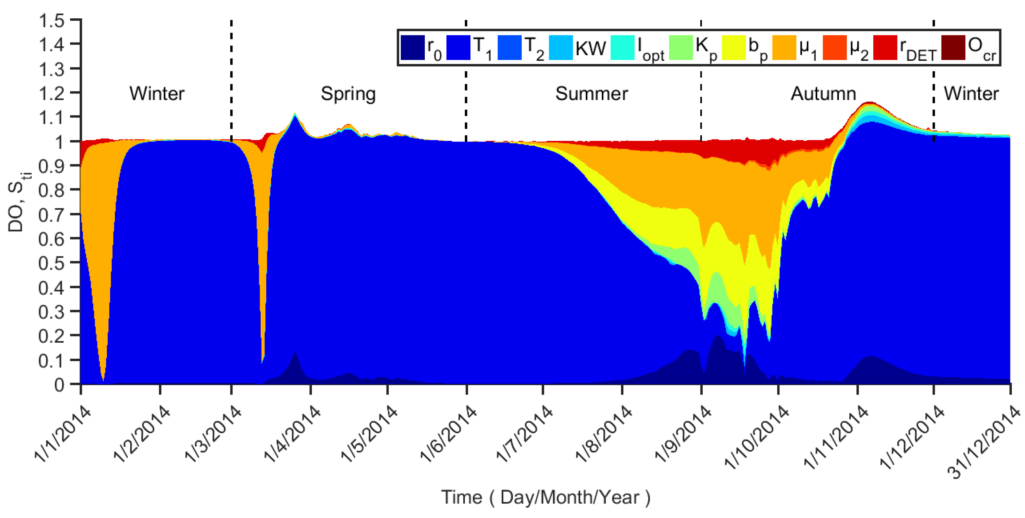
4.3. Parameter Sensitivity Temporal Variation for DO
DO concentration is also a state variable that shows the temporal variation throughout the entire time horizon (Figure 6), whereas it is different from phytoplankton. From July to November, which is from the middle summer to late autumn, the main factors are T1, μ1, bp (Phytoplankton basal respiration rate), and rDET (Detritus remineralization rate). The summation over these four parameters explains around 93% of DO concentration variance. The remaining parameters are irrelevant during this period. During the rest of the year, T1 and μ1 become very important parameters alternatively.
An important feature of the dynamic sensitivity analysis is that the influential parameter set changes with time, which indicates changes in the dynamic behavior of the model throughout the time horizon. As can be seen in these figures, the sum of Sti is seldom equal to 1, because the summation of the sensitivity indices is a measure of model additivity [8].
5. Discussion
5.1. Ecological Implication from Parameter Sensitivity for Chlorophyll-a
Previous studies have shown that background light attenuation, light limitation of phytoplankton growth-related parameters, and algae growth rates have been classified to be the main parameters in a number of freshwater and marine models with both local [36,37,38,39] and global [40,41] analyses. In our study, the maximum phytoplankton growth rate, the lower optimum temperature for algal growth, the phosphate half saturation constant for algae, and the phytoplankton linear mortality rate (r0, T1, Kp, and μ1) have a greater influence compared with other parameters, which indicates that the TGR tributary bay is similar to other water bodies and has difference with them as well. A GSA on Lake Dianchi [42], which is a shallow lake with an average depth of 5.2 m in China, shows that the max growth rate of algae, the basal respiration rate, the chlorophyll-a induced light extinction coefficient, and the lower bound of optimal temperature for algae have an important influence on Chlorophyll-a. These indicate that there are sufficient nutrient or no nutrient limits in Lake Dianchi. A GSA on the Paso de las Piedras Reservoir [43], which is a shallow reservoir with an average depth of 8.2 m in Argentina, shows that the most important parameters for phytoplankton are the organic phosphorus mineralization rate, phytoplankton death and respiration, and the background light attenuation coefficient. These indicate that there are also no nutrient limits due to organic phosphorus mineralization in the Paso de las Piedras Reservoir. Therefore, light is not an important parameter in the TGR compared with shallow lakes and reservoirs.
The sensitivity differences between the shallow lake and reservoir and the deep reservoir suggest that the mechanisms of nutrient supply and the nutrient cycle are different. For the large deep reservoir, due to slow changes in nutrient supplies, the algae growth rely on external loading. In this case, nutrition limits have a great influence on the Chlorophyll-a and the phosphate half saturation constant becomes an influential parameter. For the shallow lake and reservoir, changes in nutrient supplies are relatively fast, external loading and the release of internal loading may be sufficient for algae growth, and the nutrition limits have a slight influence on the Chlorophyll-a; simultaneously, other environmental conditions, such as light, become more influential to the ecological system.
Since none of the four parameters are a decisive factor, this suggests that the algae blooms in the TGR tributary bay may be caused by several factors and that its eutrophication mechanism is more complex.
5.2. Ecological Implication from Parameter Sensitivity for DO
Oxygen concentrations reflect the momentary balance between supply from photosynthesis on one hand and the metabolic processes that consume oxygen on the other. Previous studies have shown that the sensitive parameters for DO concentration are almost same as those for Chlorophyll-a in shallow lakes [42], which are the algae growth rate, the Chlorophyll-a-induced light extinction coefficient, and the lower bound of optimal temperature for algae. The most influence parameters on DO concentration are different from Chlorophyll-a in this study, and these indicate that the DO bio-chemistry processes may be different in this two-water system.
The sensitivity differences between the shallow lake or reservoir and the deep reservoir suggest that the mechanism of DO supply and the DO cycle is different. For the large deep reservoir, the oxygen consumption by organic carbon remineralization has a great influence on the DO, and at some special time in the year, the oxygen consumption cannot be neglected compared with the supply by photosynthesis and external loading. For the shallow lake, the oxygen consumption by remineralization can be neglected compared with the supply by photosynthesis and external loading; in this case, algae growth has a great influence on the DO concentration, and they have the same sensitive parameters.
6. Conclusions
In this study, Sobol’s method was applied to conduct a global sensitivity analysis for a water quality model of a TGR tributary bay. This method provides a quantitative analysis on factor sensitivity and interactions. The analysis focused on the response of chlorophyll-a and dissolved oxygen to 11 parameters. We developed the following conclusions: the results show that the chlorophyll-a is influenced mainly by the maximum phytoplankton growth rate, the lower optimum temperature for algal growth, the phosphate half saturation constant, and the phytoplankton linear mortality rate, while dissolved oxygen is influenced mainly by the maximum phytoplankton growth rate, the lower optimum temperature for algal growth, the phytoplankton basal respiration rate, and the detritus remineralization rate. Although none of these parameters can be classified as a single important parameter, the summation over the four parameters explains around 82% of chlorophyll-a and 93% of dissolved oxygen variance, respectively. The remaining parameters are irrelevant during the summer growth season. These indicate that the algae bloom in summer is a combined effect of several factors, instead of one key factor. The parameter sensitivity differences between the shallow lake and reservoir and the deep reservoir suggest that the mechanisms of the nutrient and dissolved oxygen cycles are different.
Acknowledgments
We thank the anonymous reviewers for their valuable comments, which greatly improved the manuscript. The study was financially supported by the Major Science and Technology Program for Water Pollution Control and Treatment (2012ZX07104-001), National Natural Science Foundation of China (51509066 and 51309252), and the Research Fund of the State Key Laboratory of Simulation and Regulation of Water Cycle in River Basin, China Institute of Water Resources and Hydropower Research (2016ZY04).
Author Contributions
Yao Cheng and Yuchun Wang conceived and designed the numerical experiments; Yao Cheng analyzed the results and wrote the paper; and Yuchun Wang provided data and technical help. Yajun Li and Fei Ji performed the post survey and investigation.
Conflicts of Interest
The authors declare no conflict of interest.
Appendix A
The governing equations of CB ecological water quality model are given as:
where P, DET, DO, NO3, NH4, PO4 and Si are phytoplankton, detritus, dissolved oxygen, nitrate, ammonium, phosphate, and dissolved silicon, respectively. Superscript represents the biochemistry process, subscript represents the related variables. gpp, mor, exc, res, rmn, denit, nit and upt represent gross primary production, respiration, excretion, mortality, remineralization, denitrification, nitrification and uptake.
The mathematical expression for each term in the model are given below.
Phytoplankton growth
Phytoplankton mortality
Phytoplankton excretion
Phytoplankton respiration
Detritus remineralization
Nitrification process
Phytoplankton uptake nutrients
Release nutrient process of remineralization
Release nutrient process of phytoplankton respiration
DO ecological process
Denitrification process
References
- Chen, C.; Ji, R.; Schwab, D.J.; Beletsky, D.; Fahnenstiel, G.L.; Jiang, M.; Johengen, T.H.; Vanderploeg, H.; Eadie, B.; Budd, J.W. A model study of the coupled biological and physical dynamics in Lake Michigan. Ecol. Model. 2002, 152, 145–168. [Google Scholar] [CrossRef]
- Park, K.; Jung, H.S.; Kim, H.S.; Ahn, S.M. Three-dimensional hydrodynamic-eutrophication model (HEM-3D): Application to Kwang-Yang Bay, Korea. Mar. Environ. Res. 2005, 60, 171–193. [Google Scholar] [CrossRef] [PubMed]
- Jin, K.R.; Ji, Z.G.; James, R.T. Three-dimensional water quality and SAV modeling of a large shallow lake. J. Great Lakes Res. 2007, 33, 28–45. [Google Scholar] [CrossRef]
- Wan, Y.; Ji, Z.G.; Shen, J.; Hu, G.; Sun, D. Three dimensional water quality modeling of a shallow subtropical estuary. Mar. Environ. Res. 2012, 82, 76–86. [Google Scholar] [CrossRef] [PubMed]
- Leon, L.F.; Smith, R.E.H.; Hipsey, M.R.; Bocaniov, S.A.; Higgins, S.N.; Hecky, R.E.; Antenucci, J.P.; Imberger, J.A.; Guildford, S.J. Application of a 3D hydrodynamic-biological model for seasonal and spatial dynamics of water quality and phytoplankton in lake Erie. J. Great Lakes Res. 2011, 37, 41–53. [Google Scholar] [CrossRef]
- Warren, I.R.; Bach, H.K. Mike 21: A modelling system for estuaries, coastal waters and seas. Environ. Softw. 1992, 7, 229–240. [Google Scholar] [CrossRef]
- Los, F.J.; Villars, M.T.; Van der Tol, M.W.M. A 3-dimensional primary production model (BLOOM/GEM) and its applications to the (southern) North Sea (coupled physical–chemical–ecological model). J. Mar. Syst. 2008, 74, 259–294. [Google Scholar] [CrossRef]
- Saltelli, A.; Tarantola, S.; Campolongo, F.; Ratto, M. Sensitivity Analysis in Practice: A Guide to Assessing Scientific Models; John Wiley & Sons: Hoboken, NJ, USA, 2004. [Google Scholar]
- Griensven, A.V.; Meixner, T.; Grunwald, S.; Bishop, T.; Diluzio, M.; Srinivasan, R. A global sensitivity analysis tool for the parameters of multi-variable catchment models. J. Hydrol. 2006, 324, 10–23. [Google Scholar] [CrossRef]
- Hill, M.C.; Østerby, O. Determining extreme parameter correlation in ground water models. Groundwater 2003, 41, 420–430. [Google Scholar] [CrossRef]
- Tian, W. A review of sensitivity analysis methods in building energy analysis. Renew. Sustain. Energy Rev. 2013, 20, 411–419. [Google Scholar] [CrossRef]
- Oakley, J.E.; O’Hagan, A. Probabilistic sensitivity analysis of complex models: A Bayesian approach. J. R. Stat. Soc. 2004, 66, 751–769. [Google Scholar] [CrossRef]
- Saltelli, A.; Chan, K.; Scott, E.M. Sensitivity Analysis; Wiley: New York, NY, USA, 2000. [Google Scholar]
- Saltelli, A.; Ratto, M.; Tarantola, S.; Campolongo, F. Sensitivity analysis practices: Strategies for model-based inference. Reliab. Eng. Syst. Saf. 2006, 91, 1109–1125. [Google Scholar] [CrossRef]
- Soboĺ, I.M. Quasi-monte carlo methods. Prog. Nucl. Energy 1990, 24, 55–61. [Google Scholar] [CrossRef]
- Saltelli, A.; Ratto, M.; Andres, T.; Campolongo, F.; Cariboni, J.; Gatelli, D.; Saisana, M.; Tarantola, S. Global Sensitivity Analysis: The Primer; Wiley: New York, NY, USA, 2008. [Google Scholar]
- Morris, M.D. Factorial sampling plans for preliminary computational experiments. Technometrics 1991, 33, 161–174. [Google Scholar] [CrossRef]
- Makler-Pick, V.; Gal, G.; Gorfine, M.; Hipsey, M.R.; Carmel, Y. Sensitivity analysis for complex ecological models—A new approach. Environ. Model. Softw. 2011, 26, 124–134. [Google Scholar] [CrossRef]
- Ciric, C.; Ciffroy, P.; Charles, S. Use of sensitivity analysis to identify influential and non-influential parameters within an aquatic ecosystem model. Ecol. Model. 2012, 246, 119–130. [Google Scholar] [CrossRef]
- Zheng, W.; Shi, H.; Fang, G.; Hu, L.; Peng, S.; Zhu, M. Global sensitivity analysis of a marine ecosystem dynamic model of the Sanggou Bay. Ecol. Model. 2012, 247, 83–94. [Google Scholar] [CrossRef]
- Stone, R. Three gorges dam: Into the unknown. Science 2008, 321, 628–632. [Google Scholar] [CrossRef] [PubMed]
- Ye, L.; Xu, Y.; Han, X.; Cai, Q. Daily dynamics of nutrients and chlorophyll a during a spring phytoplankton bloom in Xiangxi Bay of the three gorges reservoir. J. Freshw. Ecol. 2006, 21, 315–321. [Google Scholar] [CrossRef]
- Zhang, S.; Li, C.M.; Fu, Y.C.; Zhang, Y.; Zheng, J. Trophic states and nutrient output of tributaries bay in three gorges reservoir after impoundment. Environ. Sci. 2008, 29, 7–12. [Google Scholar]
- Liu, L.; Liu, D.; Johnson, D.M.; Yi, Z.; Huang, Y. Effects of vertical mixing on phytoplankton blooms in Xiangxi Bay of three gorges reservoir: Implications for management. Water Res. 2012, 46, 2121–2130. [Google Scholar] [CrossRef] [PubMed]
- Mao, J.; Jiang, D.; Dai, H. Spatial-temporal hydrodynamic and algal bloom modelling analysis of areservoir tributary embayment. J. Hydro-Environ. Res. 2015, 9, 200–215. [Google Scholar] [CrossRef]
- Ma, J.; Liu, D.; Wells, S.A.; Tang, H.; Ji, D.; Yang, Z. Modeling density currents in a typical tributary of the three gorges reservoir, China. Ecol. Model. 2015, 296, 113–125. [Google Scholar] [CrossRef]
- Chen, C.; Li, J.; Shen, H.; Wang, Z. Yangtze River of China: Historical analysis of discharge variability and sediment flux. Geomorphology 2001, 41, 77–91. [Google Scholar] [CrossRef]
- Nilsson, C.; Reidy, C.A.; Dynesius, M.; Revenga, C. Fragmentation and flow regulation of the world’s large river systems. Science 2005, 308, 405–408. [Google Scholar] [CrossRef] [PubMed]
- Yang, S.L.; Zhang, J.; Dai, S.B.; Li, M.; Xu, X.J. Effect of deposition and erosion within the main river channel and large lakes on sediment delivery to the estuary of the Yangtze River. J. Geophys. Res. Earth Surf. 2007, 112, 111–119. [Google Scholar] [CrossRef]
- Gordon, D.C., Jr.; Boudreau, P.R.; Mann, K.H.; Ong, J.E.; Silvert, W.L.; Smith, S.V.; Wattayakorn, G.; Wulff, F.; Yanagi, T. LOICZ Biogeochemical Modelling Guidelines; Netherlands Institute for Sea Research: Den Burg, The Netherlands, 1996. [Google Scholar]
- Bowie, G.L.; Mills, W.B.; Porcella, D.B.; Campbell, C.L.; Pagenkopf, J.R.; Rupp, G.L.; Johnson, K.M.; Chan, P.W.H.; Gherini, S.A. Rates, Constants, and Kinetics Formulations, Surface Water Quality Modeling; Environmental Protection Agency: Washington, DC, USA, 1985.
- Jørgensen, S.E.; Nielsen, S.N.; Jørgensen, L.A. Handbook of Ecological Parameters and Ecotoxicology; Elsevier: Amsterdam, The Netherlands, 1991; Volume 29, p. 791. [Google Scholar]
- Chen, C.; Ji, R.; Zheng, L.; Zhu, M.; Rawson, M. Influences of physical processes on the ecosystem in Jiaozhou Bay: A coupled physical and biological model experiment. J. Geophys. Res. Oceans 1999, 104, 29925–29930. [Google Scholar] [CrossRef]
- Cannavó, F. Sensitivity analysis for volcanic source modeling quality assessment and model selection. Comput. Geosci. 2012, 44, 52–59. [Google Scholar] [CrossRef]
- Baklouti, M.; Faure, V.; Pawlowski, L.; Sciandra, A. Investigation and sensitivity analysis of a mechanistic phytoplankton model implemented in a new modular numerical tool (Eco3M) dedicated to biogeochemical modelling. Prog. Oceanogr. 2006, 71, 34–58. [Google Scholar] [CrossRef]
- Bierman, V.J.; James, R.T. A preliminary modeling analysis of water quality in Lake Okeechobee, Florida: Diagnostic and sensitivity analyses. Water Res. 1995, 29, 2767–2775. [Google Scholar] [CrossRef]
- Omlin, M.; Reichert, P.; Forster, R. Biogeochemical model of Lake Zürich: Model equations and results. Ecol. Model. 2001, 141, 77–103. [Google Scholar] [CrossRef]
- Chu, P.C.; Ivanov, L.M.; Margolina, T.M. On non-linear sensitivity of marine biological models to parameter variations. Ecol. Model. 2007, 206, 369–382. [Google Scholar] [CrossRef]
- Fragoso, J.C.R.; Marques, D.M.L.M.; Collischonn, W.; Tucci, C.E.M.; Nes, E.H.V. Modelling spatial heterogeneity of phytoplankton in Lake Mangueira, a large shallow subtropical lake in South Brazil. Ecol. Model. 2008, 219, 125–137. [Google Scholar] [CrossRef]
- Arhonditsis, G.B.; Brett, M.T. Eutrophication model for Lake Washington (USA): Part I. Model description and sensitivity analysis. Ecol. Model. 2005, 187, 140–178. [Google Scholar] [CrossRef]
- Guven, B.; Howard, A. Identifying the critical parameters of a cyanobacterial growth and movement model by using generalised sensitivity analysis. Ecol. Model. 2007, 207, 11–21. [Google Scholar] [CrossRef]
- Yi, X.; Zou, R.; Guo, H. Global sensitivity analysis of a three-dimensional nutrients-algae dynamic model for a large shallow lake. Ecol. Model. 2016, 327, 74–84. [Google Scholar] [CrossRef]
- Estrada, V.; Diaz, M.S. Global sensitivity analysis in the development of first principle-based eutrophication models. Environ. Model. Softw. 2010, 25, 1539–1551. [Google Scholar] [CrossRef]
Figure 1.
Study area and sampling sites. YR: Yangtze River.
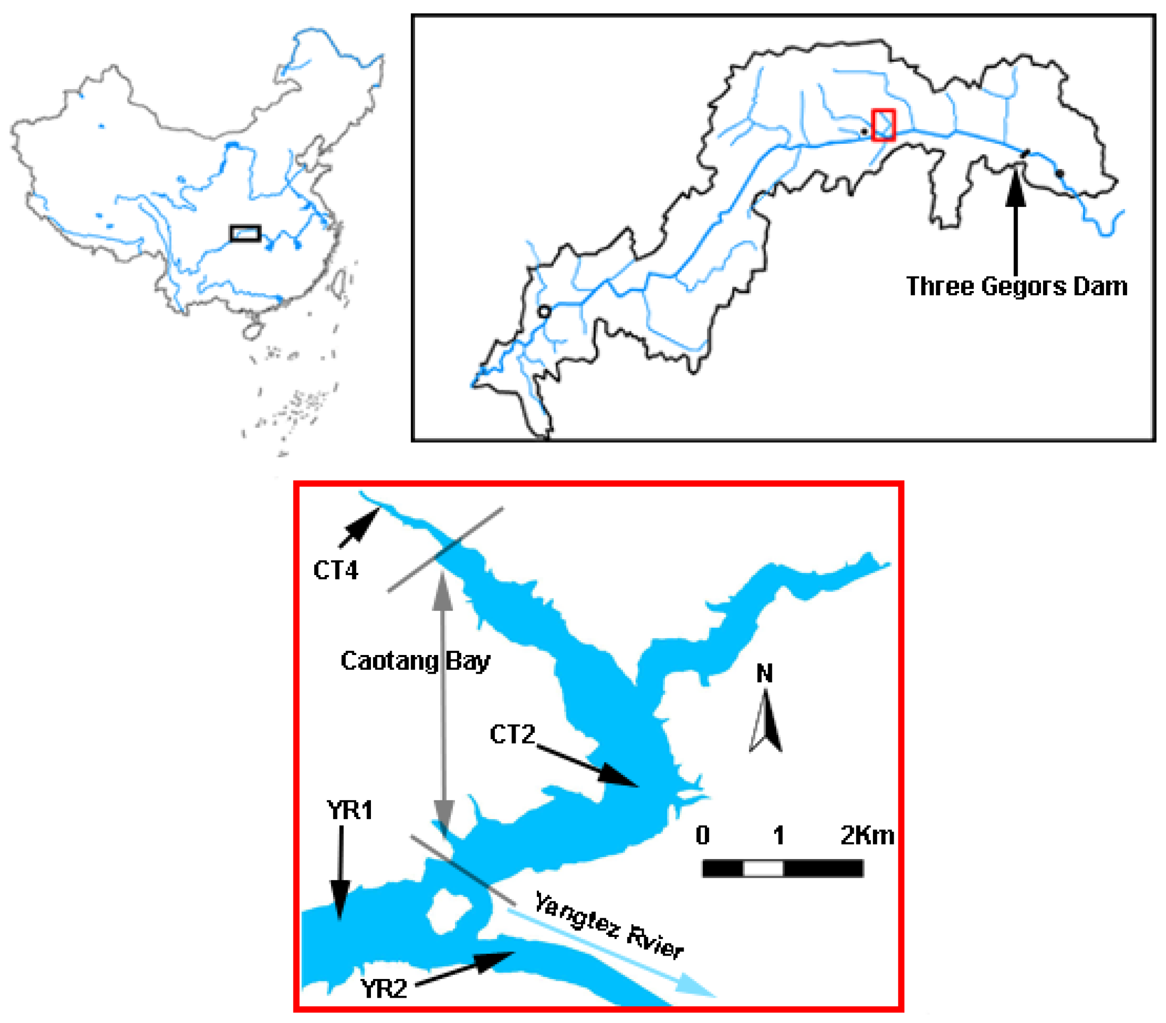
Figure 2.
Generalized box diagram illustrating the budget for water and material.
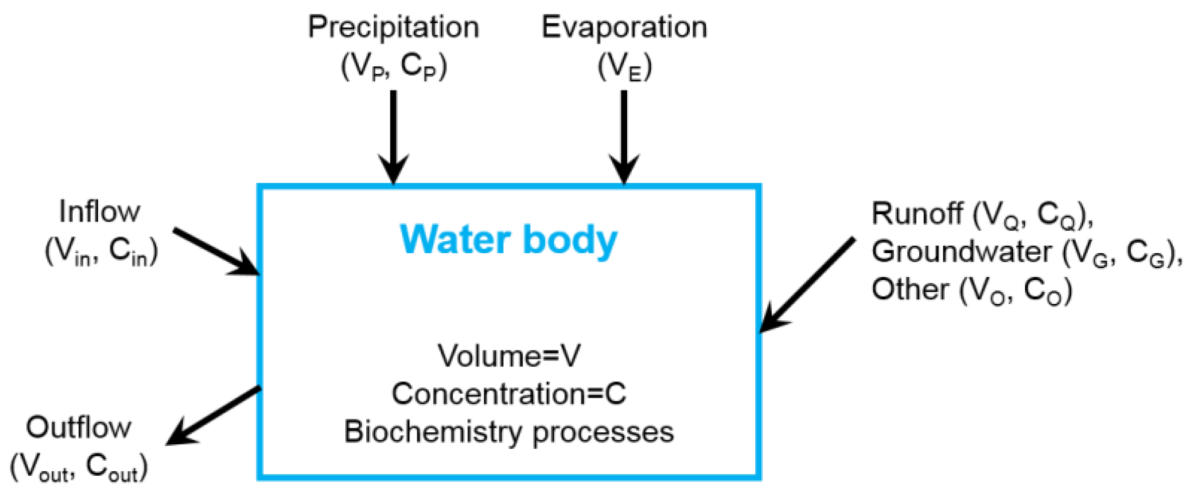
Figure 3.
Schematic of the water quality model in TGR. P, DET, DO, NO3, NH4, PO4 and Si are phytoplankton, detritus, dissolved oxygen, nitrate, ammonium, phosphate, and dissolved silicon, respectively.
Figure 3.
Schematic of the water quality model in TGR. P, DET, DO, NO3, NH4, PO4 and Si are phytoplankton, detritus, dissolved oxygen, nitrate, ammonium, phosphate, and dissolved silicon, respectively.
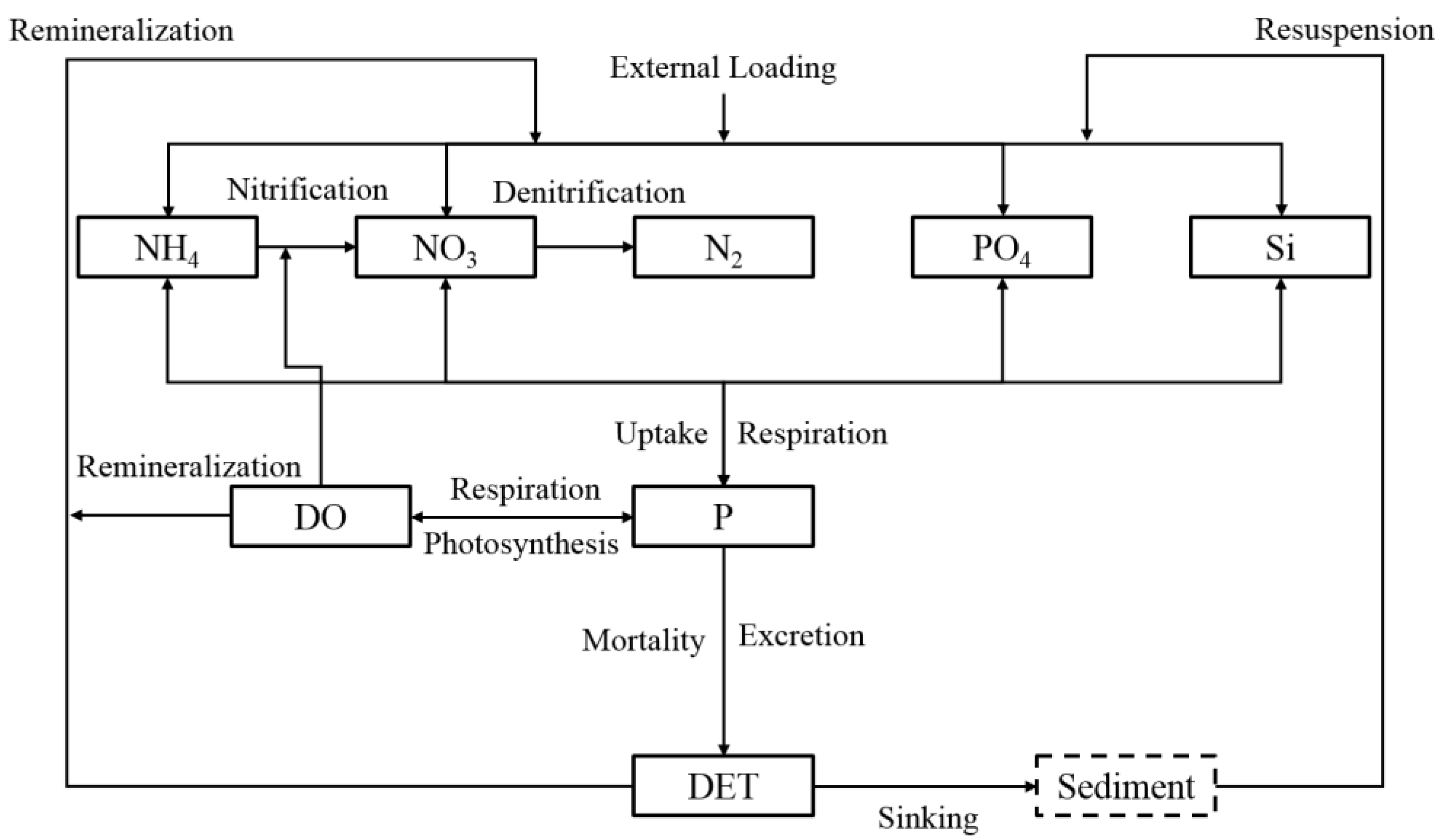
Figure 4.
Sti profiles for Chlorophyll-a concentration and dissolved oxygen (DO).
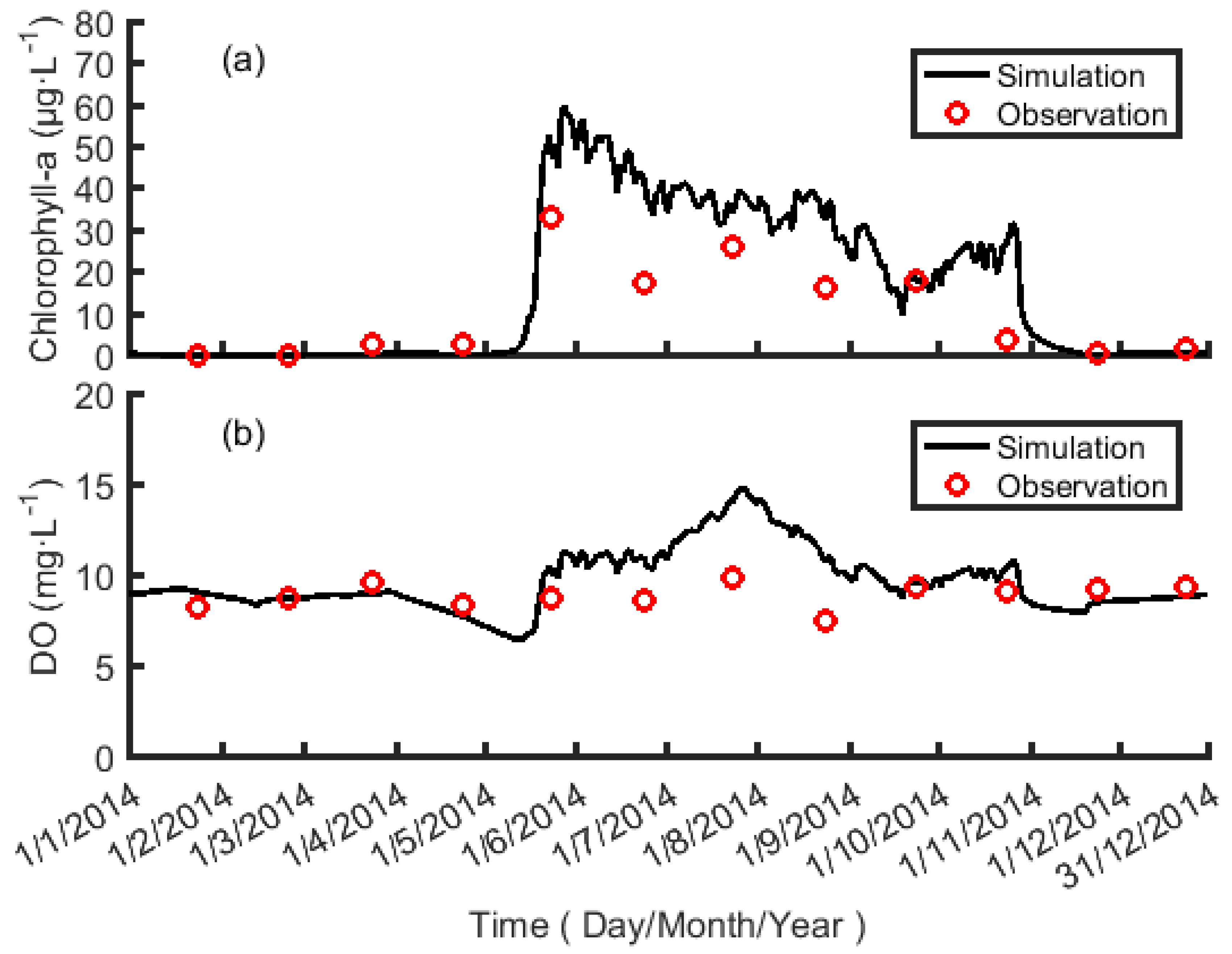
Figure 5.
Sti profiles for Chlorophyll-a concentration.
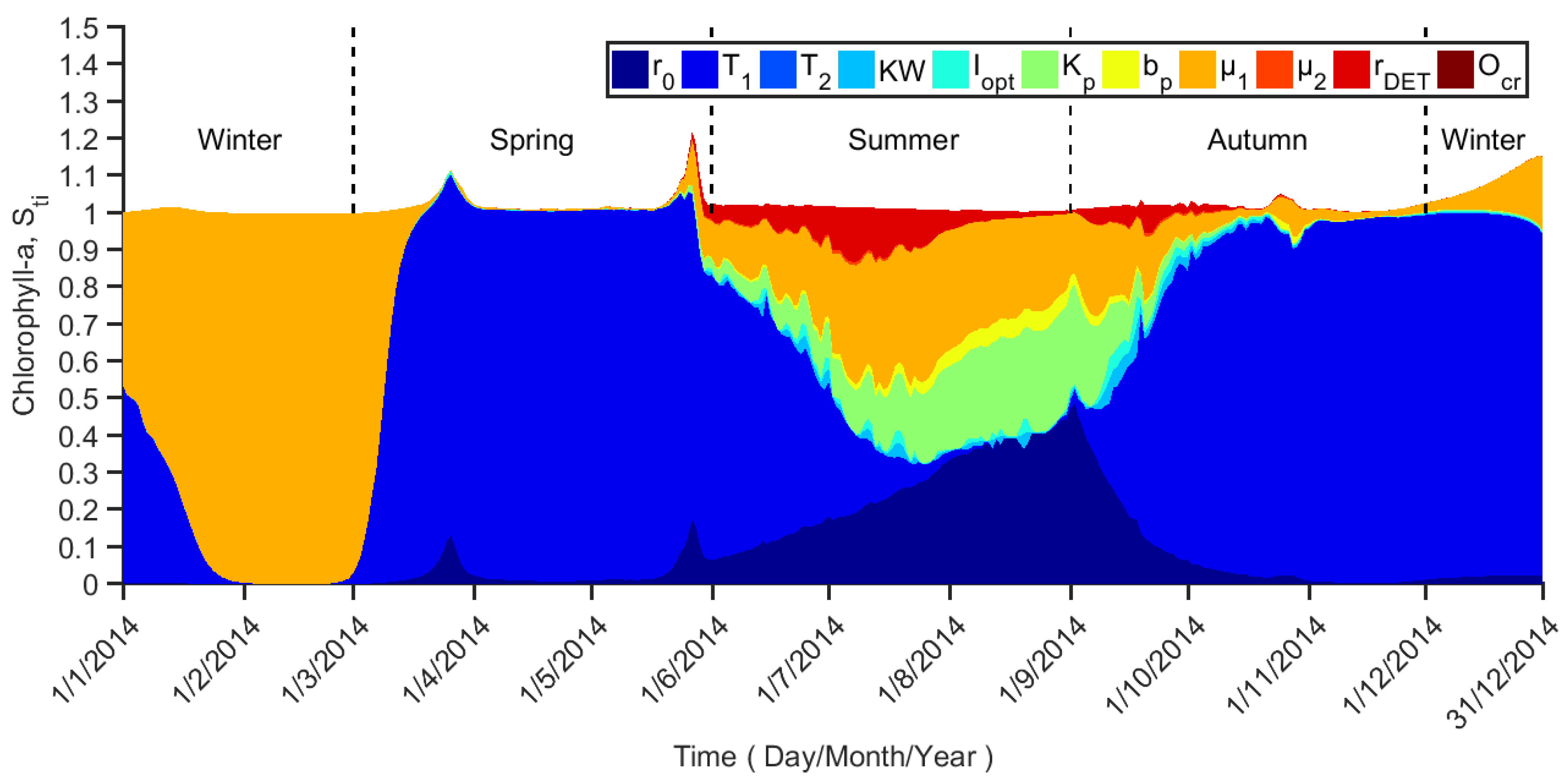
Figure 6.
Sti profiles for DO concentration.


Table 1.
The parameter values of the ecological water quality model applied in the Caotang Bay (CB).
Table 1.
The parameter values of the ecological water quality model applied in the Caotang Bay (CB).
| Parameter | Description | Value | Unit | Selected to GSA (Y/N) |
|---|---|---|---|---|
| Maximum phytoplankton growth rate | 3.039 | day−1 | Y | |
| Lower optimum temperature for algal growth | 24 | °C | Y | |
| Upper optimum temperature for algal growth | 29 | °C | Y | |
| Light extinction coefficient for all absorption components (except algae) | 1 | m−1 | Y | |
| Factor for light extinction coefficient for algae | 0.01 | m−1 mmolC−1 | N | |
| Optimum light intensity | 80.0 | W m−2 | Y | |
| Nitrate half saturation constant for algae | 0.040 | mmolN m−3 | N | |
| Ammonia half saturation constant for algae | 0.030 | mmolN m−3 | N | |
| Phosphate half saturation constant for algae | 0.285 | mmolP m−3 | Y | |
| Silica half saturation constant for algae | 1.16 | mmolSi m−3 | N | |
| Phytoplankton linear mortality rate | 0.335 | day−1 | Y | |
| Phytoplankton second order mortality rate | 0.001 | mmolC day−1 | Y | |
| Phytoplankton excretion rate | 0.15 | day−1 | N | |
| Phytoplankton basal respiration rate | 0.2 | day−1 | Y | |
| Phytoplankton active respiration rate | 0.1 | day−1 | N | |
| Oxygen critical concentration for nitrification | 11.161 | mmolO2 m−3 | Y | |
| Oxygen confinement factor for nitrification | 6.0 | -- | N | |
| Detritus remineralization rate | 0.127 | day−1 | Y | |
| Temperature confinement factor for remineralization | 20.0 | -- | N | |
| Reference temperature for remineralization | 13.0 | °C | N | |
| Nitrification rate | 0.045 | day−1 | N | |
| Denitrification rate | 0.01 | mmolN m−3 day−1 | N | |
| Detritus half saturation constant | 6.625 | mmolC m−3 | N | |
| Denitrification ratio of detritus | 1.25 | -- | N | |
| Ammonia release ratio for denitrification | 0.189 | -- | N | |
| Phosphate release ratio for denitrification | 0.012 | -- | N | |
| Silica release ratio for denitrification | 0.259 | -- | N | |
| Redfield ratio P:C | 1:106 | -- | N | |
| Redfield ratio N:C | 16:106 | -- | N | |
| Redfield ratio Si:C | 22:106 | -- | N | |
| Stoichiometric number of carbon to oxygen | 1 | mmolO2 mmolC−1 | N | |
| Stoichiometric number of nitrogen to oxygen | 2 | mmolO2 mmolN−1 | N |
GSA: global sensitivity analysis.
Table 2.
Notations used in the text.
| Symbol | Description |
|---|---|
| N | Sample size |
| k | Number of factors |
| Xi | Generic factor |
| X | N × k matrix of input factors |
| N × (k − 1) matrix of all factors but Xi | |
| , | Variance or mean of argument (·) taken over Xi |
| , | Variance or mean of argument (·) taken over all factors but Xi |
Table 3.
Relevance of an input parameter from its global sensitivity index.
| Condition | Description |
|---|---|
| 0.8 ≤ Sti ≤ 1 | Very important |
| 0.5 ≤ Sti < 0.8 | Important |
| 0.3 ≤ Sti < 0.5 | Unimportant |
| 0 ≤ Sti < 0.3 | Irrelevant |
© 2018 by the authors. Licensee MDPI, Basel, Switzerland. This article is an open access article distributed under the terms and conditions of the Creative Commons Attribution (CC BY) license (http://creativecommons.org/licenses/by/4.0/).
Share and Cite
MDPI and ACS Style
Cheng, Y.; Li, Y.; Ji, F.; Wang, Y. Global Sensitivity Analysis of a Water Quality Model in the Three Gorges Reservoir. Water 2018, 10, 153. https://doi.org/10.3390/w10020153
AMA Style
Cheng Y, Li Y, Ji F, Wang Y. Global Sensitivity Analysis of a Water Quality Model in the Three Gorges Reservoir. Water. 2018; 10(2):153. https://doi.org/10.3390/w10020153
Chicago/Turabian StyleCheng, Yao, Yajun Li, Fei Ji, and Yuchun Wang. 2018. "Global Sensitivity Analysis of a Water Quality Model in the Three Gorges Reservoir" Water 10, no. 2: 153. https://doi.org/10.3390/w10020153
Note that from the first issue of 2016, this journal uses article numbers instead of page numbers. See further details here.