Implementation of Extended Statistical Entropy Analysis to the Effluent Quality Index of the Benchmarking Simulation Model No. 2

Abstract
:1. Introduction
2. Materials and Methods
2.1. The Simulation of WWT According to the BSM No. 2 Setup Including the Modeling of GHG Emissions

| Influent, Wastewater type | WW inflow m3/day | Concentration in the wastewater | ||||||
|---|---|---|---|---|---|---|---|---|
| BOD g/m3 | COD g/m3 | SS g/m3 | NH 4+g N/m3 | SBN g N/m3 | PBN g N/m3 | Total N-load kgN/day | ||
| I | 861 | 301 | 587 | 54.7 | 26.8 | 6.4 | 18.5 | 44.5 |
| II | 864 | 274 | 524 | 151 | 35.3 | 2.52 | 2.52 | 34.9 |
| III | 528 | 110 | 213 | 21.3 | 15.3 | 1.31 | 3.40 | 10.6 |
| Simulation (#) | Influent, Wastewater type | Aeration tank (mgO2/L) | ||
|---|---|---|---|---|
| 1 | 2 | 3 | ||
| 1 | I | 1 | 1 | 1 |
| 2 | 2 | 2 | 2 | |
| 3 | II | 1 | 1 | 1 |
| 4 | 2 | 2 | 2 | |
| 5 | III | 1 | 1 | 1 |
| 6 | 2 | 2 | 2 | |
2.2. Effluent Quality Index (EQ) Used in BSM No. 2

2.3. Extended Statistical Entropy Analysis (eSEA)
2.3.1. General Remarks
2.3.2. Calculation Path


 and the corresponding concentration term
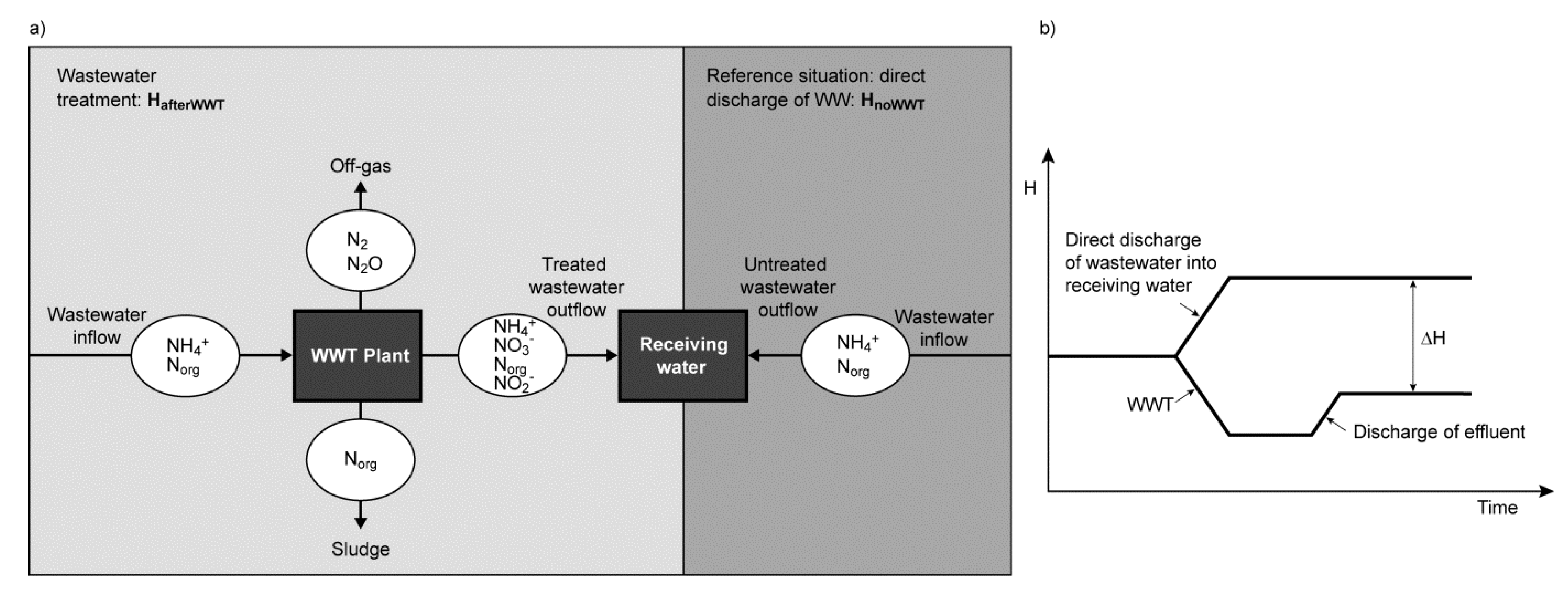
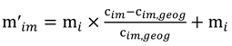
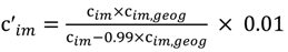
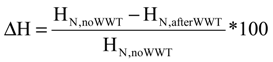
  are calculated according to Equations (4) and (5), respectively. The mass-function calculates how much mass in the water or air is needed to dilute the emitted concentration to its corresponding background concentration. The dimensionless mass-function for the N in the sludge is computed according to Equation (2). The statistical entropy, H, is then calculated according to Equation (6). Thus, the statistical entropy is a function of the mass flows, such as the wastewater, effluent, off-gas and sludge, the emission concentrations and the corresponding background concentrations of all N-compounds. More diluted mass flows and larger differences between the emitted and the background concentrations result in higher entropy values and, consequently, increased dilution in the environment. Given the assumption that for sustainable resource management dilution should be avoided whenever possible, low entropy values are desired. For a more detailed description of how to apply eSEA to processes, see [30]. Statistical entropy is calculated for the direct discharge of the wastewater to the receiving waters (HnoWWT) (Figure 1a right) and for the discharge of the treated wastewater including the N-transfer to the sludge and to the off-gas (HafterWWT) (cf. Figure 1a left). Both entropy values (HnoWWT and HafterWWT) indicate the distribution of the different N-compounds in the receiving water, the atmosphere, and the sludge. The difference between HnoWWT and HafterWWT is the reduction in statistical entropy, ∆H, and equals the benefit of the particular WWTP. Figure 1b highlights that WWT is certainly preferential to the direct discharge of the wastewater to the river because it will cause less dilution, which is expressed by less entropy production. The higher ΔH is the greater is the benefit of the particular WWTP with respect to N-treatment. A detailed description of the calculation and the application of eSEA to WWTPs can be found in [30,32].
3. Results and Discussion
3.1. The Implementation of eSEA as to the EQ

3.2. Comparison of the Traditional EQ and the New Defined EQ
| Simulation# | N2O | EQIN kgPU/day | EQOUT kgPU/day | ΔEQ % | ΔEQrest % | ΔEQN % | ΔN % | ΔH % | ΔEQnew % | |
|---|---|---|---|---|---|---|---|---|---|---|
| kgN-N2O/day | %NIN | |||||||||
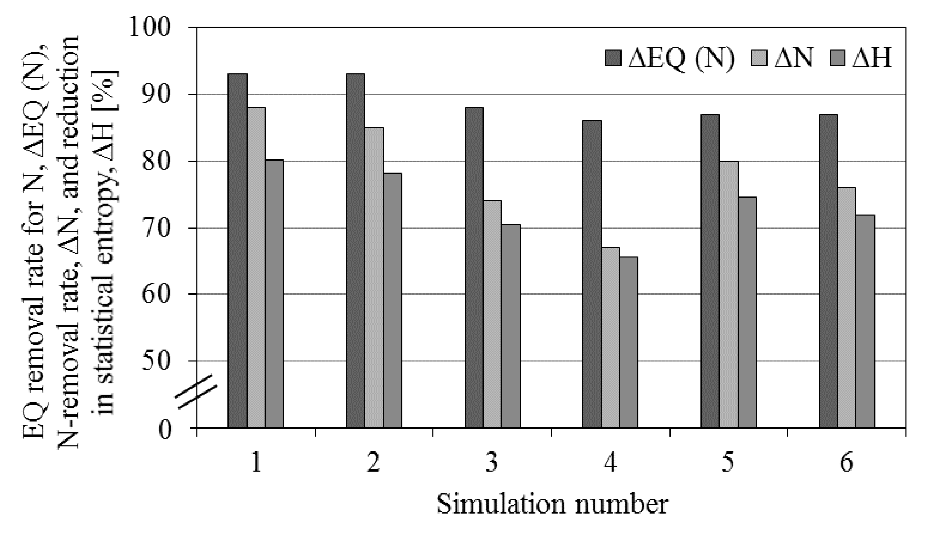
| 1 | 3.3 | 0.35 | 58,878 | 4,203 | 93 | 93 | 93 | 88 | 81 | 82 |
| 2 | 3.2 | 0.34 | 4,379 | 93 | 93 | 93 | 85 | 79 | 80 | |
| 3 | 3.7 | 0.44 | 53,571 | 4,682 | 91 | 94 | 88 | 74 | 71 | 73 |
| 4 | 3.4 | 0.41 | 5,230 | 90 | 94 | 86 | 67 | 66 | 68 | |
| 5 | 0.98 | 0.39 | 13,630 | 1,640 | 88 | 89 | 87 | 80 | 75 | 76 |
| 6 | 0.94 | 0.37 | 1,629 | 88 | 90 | 87 | 76 | 72 | 73 | |
| N-compound | Load (kgN/day) for Simulation # | |||||
|---|---|---|---|---|---|---|
| 1 | 2 | 3 | 4 | 5 | 6 | |
| N-NO3− | 3.7 | 4.8 | 7.2 | 10 | 1.1 | 1.8 |
| N-NH4+ | 0.17 | 8.7 × 10⁻² | 0.31 | 0.16 | 0.45 | 0.21 |
| SBN | 1.7 | 1.6 | 1.6 | 1.5 | 0.59 | 0.58 |
| PBN | 2.6 × 10⁻² | 2.6 × 10⁻² | 2.6 × 10⁻² | 2.6 × 10⁻² | 5.3 × 10⁻³ | 4.7 × 10⁻³ |
| TKN | 1.9 | 1.8 | 1.7 | 1.9 | 1.1 | 0.8 |
| N-compound | Concentration (gN/m3) for Simulation # | Natural background concentration | |||||
|---|---|---|---|---|---|---|---|
| 1 | 2 | 3 | 4 | 5 | 6 | ||
| N-NO3− | 4.3 | 5.6 | 8.3 | 12 | 2.0 | 3.4 | 1.0–4.0 (1) |
| N-NH4+ | 0.20 | 0.10 | 0.36 | 0.18 | 0.85 | 0.40 | 0.01–0.05 (2) |
| SBN | 1.9 | 1.89 | 1.8 | 1.8 | 1.1 | 1.1 | 0.1–0.4 (2) |
| PBN | 3.0 × 10⁻² | 3.0 × 10⁻² | 3.0 × 10⁻² | 3.0 × 10⁻² | 1 × 10⁻² | 1 × 10⁻² | 0.1–0.4 (2) |
| TKN | 2.2 | 2.0 | 2.2 | 2.0 | 2.0 | 1.5 | - |
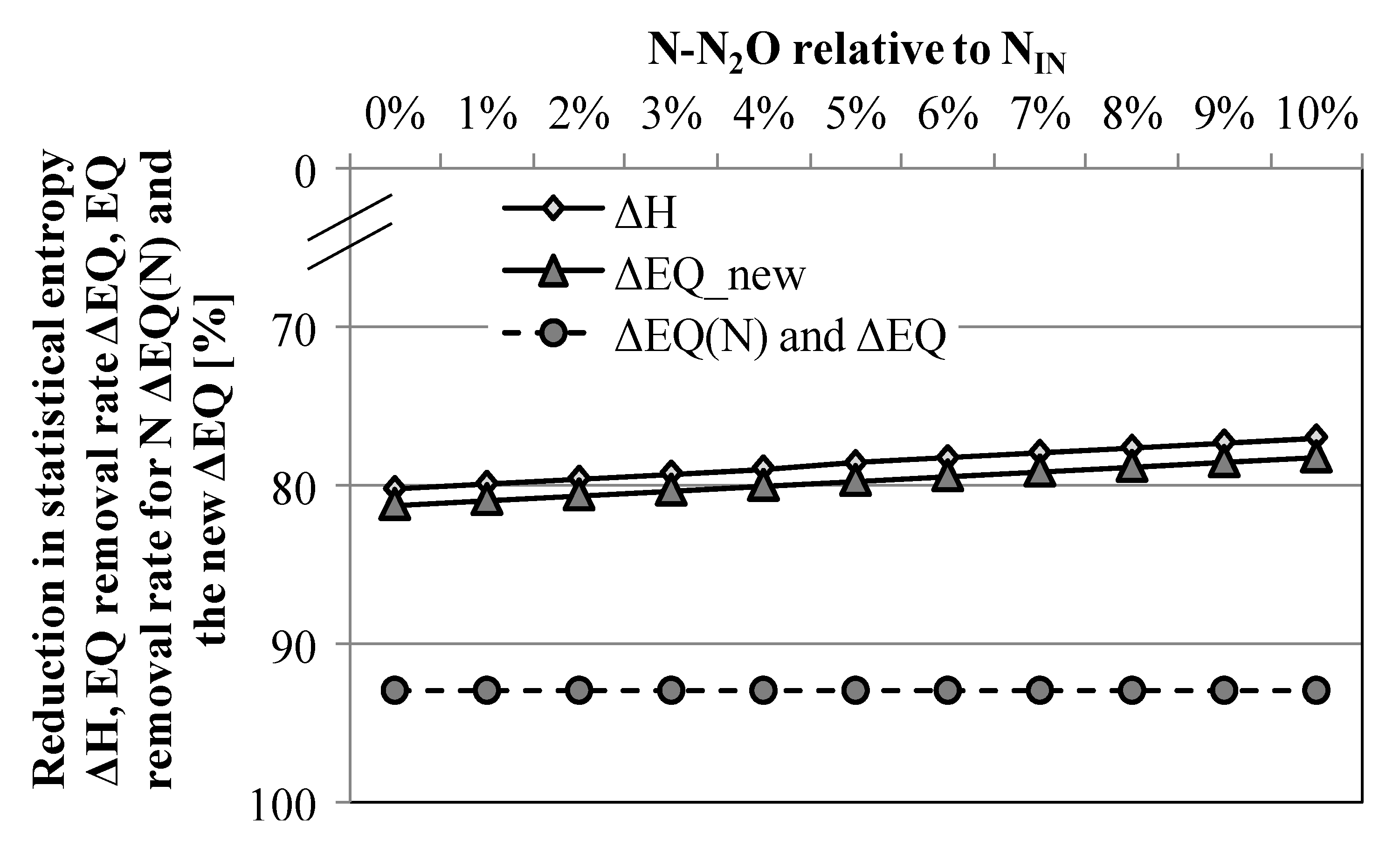
3.3. Scenario Analysis: Relevance of N2O for the Overall N-Performance

4. Conclusions
Acknowledgments
Conflicts of Interest
References
- Jeppsson, U.; Pons, M.-N.; Nopens, I.; Alex, J.; Copp, J.B.; Gernaey, K.V.; Rosen, C.; Steyer, J.-P.; Vanrollehghem, P.A. Benchmark simulation model No. 2: General protocol and exploratory case studies. Water Sci. Technol. 2007, 56, 67–78. [Google Scholar]
- IPCC, Climate Change 2001: The Scientific Basis. In Atmosferic Chemistry and Greenhouse Gases; UNEP GRID-Ardenal: Ardenal, Norway, 2001; Chapter 4.
- Gupta, D.; Singh, S.K. Greenhouse gas emissions from wastewater treatment plants: A case study of noida. J. Water Sustain. 2012, 2, 131–139. [Google Scholar]
- Kampschreur, M.J.; Temmink, H.; Kleerebezem, R.; Jetten, M.S.M.; van Loosdrecht, M.C.M. Nitrous oxide emission during wastewater treatment. Water Res. 2009, 43, 4093–4103. [Google Scholar] [CrossRef]
- Lolito, A.M.; Wunderlin, P.; Joss, A.; Kipf, M.; Siegrist, H. Nitrous oxide emissions from the oxidation tank of a pilot activated sludge plant. Water Res. 2012, 46, 3563–3573. [Google Scholar] [CrossRef]
- Goreau, T.J.; Kaplan, W.A.; Wofsy, S.C.; McElroy, M.B.; Valois, F.W.; Watson, S.W. Production of nitrite and nitrogen oxide (N2O) by nitrifying bacteria at reduced concentrations of oxygen. Appl. Environ. Microbiol. 1980, 40, 526–532. [Google Scholar]
- Dumit, M.; Gabarro, J.; Murthy, S.; Riffat, R.; Wett, B.; Colprim, J.; Chandran, K. The Impact of Post Anoxic Dissolved Oxygen Concentrations on Nitrous Oxide Emissions in Nitrification Processes. In Proceedings of the 84th Annual Water Environment Federation Technical Exhibition and Conference,, Los Angeles,CA, USA, 15–19 October 2011; Water Environment Federation: Alexandria, VA, USA, 2011. [Google Scholar]
- Hu, Z.; Zhang, J.; Xie, H.; Li, S.; Wang, J.; Zhang, T. Effect of anoxic/aerobic phase fraction on N2O emission in a sequencing batch reactor under low temperature. Bioresour. Technol. 2011, 102, 5486–5491. [Google Scholar] [CrossRef]
- Aboobakar, A.; Cartmell, E.; Stephenson, T.; Jones, M.; Vale, P.; Dotro, G. Nitrous oxide emissions and dissolved oxygen profiling in a full-scale nitrifying activated sludge treatment plant. Water Res. 2012, 47, 524–534. [Google Scholar]
- Winter, P.; Pearce, P.; Colquhoun, K. Contributions of nitrous oxide emissions form wastewater treatment to carbon accounting. J. Water Clim. Chang. 2012, 3, 95–109. [Google Scholar] [CrossRef]
- Jia, W.; Liang, S.; Zhang, J.; Ngo, H.H.; Guo, W.; Yan, Y.; Zou, Y. Nitrous oxide emission in low-oxygen simultaneous nitrification and denitrification process: Sources and mechanisms. Bioresour. Technol. 2013. [Google Scholar] [CrossRef]
- Flores-Alsina, X.; Corominas, L.; Snip, L.; Vanrolleghem, P.A. Including greenhouse gas emissions during benchmarking of wastewater treatment plant control strategies. Water Res. 2011, 45, 4700–4710. [Google Scholar]
- Snip, L. Quantifying the Greenhouse Gas Emissions of Wastewater Treatment Plants. Master’s Thesis, Department of Agrotechnology and Food Science,Wageningen University, Wageningen, The Netherland, 2010. [Google Scholar]
- Rodriguez-Garcia, G.; Hospido, A.; Bagley, D.M.; Moreira, M.T.; Feijoo, G. A methodology to estimate greenhouse gases emissions in Life Cycle Inventories of wastewater treatment plants. Environ. Impact Assess. Rev. 2012, 37, 37–46. [Google Scholar] [CrossRef]
- Corominas, L.; Flores-Alsina, X.; Snip, L.; Vanrolleghem, P.A. Comparison of different modeling approaches to better evaluate greenhouse gas emissions from whole wastewater treatment plants. Biotechnol. Bioeng. 2012. [Google Scholar] [CrossRef]
- Yu, R.; Kampschreur, M.J.; van Loosdrecht, M.C.M.; Chandran, K. Mechanisms and specific directionality of autotrophic nitrous oxide and nitric oxide generation during transient anoxia. Environ. Sci. Technol. 2010, 44, 1313–1319. [Google Scholar] [CrossRef]
- Wunderlin, P.; Lehmann, M.F.; Siegrist, H.; Tuzson, B.; Joss, A.; Emmenegger, L.; Mohn, J. Isotope signatures of N2O in a mixed microbial population system: Constraints on N2O producing pathways in wastewater treatment. Environ. Sci. Technol. 2013, 47, 1339–1348. [Google Scholar]
- Zhang, T.T.; Zhang, J.; Yang, F.; Xie, H.J.; Hu, Z.; Li, Y.R. Effect of temperature on pollutant removal and nitrous oxide emissions of wastewater nitrogen removal system. US Natl. Cent. Biotechnol. Inf. 2012, 33, 1283–1287. [Google Scholar]
- Law, Y.; Lant, P.; Yuan, Z. The effect of pH on N2O production under aerobic conditions in a partial nitritation system. Water Res. 2011, 45, 5934–5944. [Google Scholar] [CrossRef]
- Zhu, X.; Chen, Y.; Chen, H.; Li, X.; Peng, Y.; Wang, S. Minimizing nitrous oxide in biological nutrient removal from municipal wastewater by controlling copper ion concentrations. Appl. Microbiol. Biotechnol. 2013, 97, 1325–1334. [Google Scholar] [CrossRef]
- Daelman, M.R.J.; van Voorthuizen, E.M.; van Dongen, L.G.J.M.; Volcke, E.I.P.; van Loosdrecht, M.C. Methane and nitrous oxide emissions from municipal wastewater treatment—Results from a long-term study. Water Sci. Technol. 2013, 67, 2350–2355. [Google Scholar] [CrossRef]
- Shaw, A.R.; Ko, S.-H. Gaseous emissions from wastewater facilities. Water Environ. Res. 2012, 84, 1325–1331. [Google Scholar] [CrossRef]
- Hiatt, W.C.; Grady, C.P.L., Jr. Application of the activated sludge model for nitrogen to elevated nitrogen conditions. Water Environ. Res. 2008, 80, 2134–2144. [Google Scholar] [CrossRef]
- Nopens, I.; Benedetti, L.; Jeppsson, U.; Pons, M.-N.; Alex, J.; Copp, J.B.; Gernaey, K.V.; Rosen, C.; Steyer, J.-P.; Vanrolleghem, P.A. Benchmark simulation model No 2: Finalisation of plant layout and default control strategy. Water Sci. Technol. 2010, 62, 1967–1974. [Google Scholar] [CrossRef]
- Vanrolleghem, P.A.; Gillot, S. Robustness and economic measures as control benchmark performance criteria. Water Sci. Technol. 2002, 45, 117–126. [Google Scholar]
- Haemelinck, S. Evaluatie van sturingsalgoritmen voor de verwijdering van stikstof uit afvalwater (Evaluation of Control Algorithms for Nitrogen Removal from Wastewaters). Engineers Thesis, Ghent University, Gent, Belgium, 2000. [Google Scholar]
- Yuan, L.M.; Zhang, C.Y.; Yan, R.; Zhao, G.Z.; Tian, L.J.; He, Z.X.; Liu, H.; Zhang, Y.Q. Advanced wastewater treatment under different dissolved oxygen conditions in an innovative step-feed process. Adv. Mater. Res. 2012, 383–390, 3707–3712. [Google Scholar]
- Coen, F.; Vanderhaegen, B.; Boonen, I.; Vanrolleghem, P.A.; van Eyck, L.; van Meenen, P. Nitrogen removal upgrade of a wastewater treatment plant within existing reactor volumes: A simulation supported scenario analysis. Water Sci. Technol. 1996, 34, 339–346. [Google Scholar]
- Kessler, R. Stormwater strategies cities prepare aging infrastructure for climate change. Environ. Health Perspect. 2011, 119, 516–519. [Google Scholar]
- Sobańtka, A.P.; Zessner, M.; Rechberger, H. Extension of statistical entropy analysis to chemical compounds. Entropy 2012, 14, 2413–2426. [Google Scholar] [CrossRef]
- Sobańtka, A.P.; Thaler, S.; Zessner, M.; Rechberger, H. Extended statistical entropy analysis for the evaluation of nitrogen budgets in Austria. Int. J. Environ. Sci. Technol. 2013. [Google Scholar] [CrossRef]
- Sobańtka, A.P.; Rechberger, H. Extended statistical entropy analysis (eSEA) for improving evaluation of wastewater treatment plants (WWTPs). Water Sci. Technol. 2013, 67, 1051–1057. [Google Scholar]
- Ahn, J.H.; Kim, S.; Park, H.; Rahm, B.; Pagilla, K.; Chandran, K. N2O emissions from activated sludge processes, 2009–2009: Results of a national monitoring survey in the United States. Environ. Sci. Technol. 2010, 44, 4505–4511. [Google Scholar]
- Vanrolleghem, P.A.; Jeppsson, U.; Cartensen, J.; Carlsson, B.; Olsson, G. Integration of wastewater treatment plant design and operation—A systematic approach using cost functions. Water Sci. Technol. 1996, 34, 159–171. [Google Scholar]
- Tyagi, V.K.; Chopra, A.K.; Durgapal, N.C.; Kuar, A. Evaluation of daphnia magna as an indicator of toxicity and treatment efficacy of municipal sewage treatment plant. J. Appl. Sci. Environ. Manag. 2007, 11, 61–67. [Google Scholar]
- Heijungs, R.; Guinée, J.B.; Huppes, G.; Lankreijer, R.M.; Udo de Haes, H.A.; Sleeswijk, A.W. 1992 Environmental Life Cycle Assessment of Products—Backgrounds; Centre of Environmental Science: Leiden, The Netherlands, 1992. [Google Scholar]
- Goedkoop, M.; Spriensma, R. The Eco-Indicator 99 A Damage Oriented Method for Life Cycle Impact Assessment; PRé Consultants B.V.: Amersfoort, The Netherlands, 2000. [Google Scholar]
- Guinée, J.B.; Gorée, M.; Heijungs, R.; Huppes, G.; Kleijn, R.; de Koning, A.; van Wegener Oers, L.; Sleeswijk, A.; Suh, S.; Udo de Haes, H.A.; et al. 2002 Handbook on Life Cycle Assessment. Operational Guide to the ISO Standards. I: LCA in Perspective. IIa: Guide. IIb: Operational Annex. III: Scientific Background; Kluwer Academic Publishers: Dordrecht, The Netherlands, 2002; p. 692, ISBM:1-4020-0228-9. [Google Scholar]
- Pennington, D.W.; Margni, M.; Amman, C.; Jolliet, O. Spatial versus non-spatial multimedia fate and exposure modeling: Insights for Western Europe. Environ. Sci. Technol. 2005, 39, 1119–1128. [Google Scholar] [CrossRef]
- Pennington, D.W.; Margni, M.; Payet, J.; Jolliet, O. Risk and regulatory hazard based toxicological effect indicators in Life Cycle Assessment (LCA). Hum. Ecotoxicol. Risk Assess. J. 2006, 12, 450–475. [Google Scholar] [CrossRef]
- Rechberger, H.; Brunner, P.H. A new, entropy based method to support waste and resource management decisions. Environ. Sci. Technol. 2002, 34, 809–816. [Google Scholar] [CrossRef]
- Shannon, C.E. A mathematical theory of communication. Bell Syst. Technol. J. 1948, 27, 623–656. [Google Scholar] [CrossRef]
- Tai, S.; Goda, T. Entropy analysis of water and wastewater treatment processes. Int. J. Environ. Stud. 1985, 25, 13–21. [Google Scholar] [CrossRef]
- Larsen, T.; Gujer, W. The concept of sustainable urban water management. Water Sci. Technol. 1997, 35, 3–10. [Google Scholar] [CrossRef]
- Kampschreur, M.J.; van der Star, W.R.L.; Wielders, H.A.; Mulder, J.W.; Jetten, M.S.M.; van Loosdrecht, M.C.M. Dynamics of nitric oxide and nitrous oxide emissions during full-scale reject water treatment. Water Res. 2008, 42, 812–826. [Google Scholar] [CrossRef]
- Verordnung des Bundesministers für Land-und Forstwirtschaft, Umwelt und Wasserwirtschaft über die Festlegung des ökologischen Zustandes für Oberflächengewässer Teil II (Austrian Quality Objective Ordinance—Ecological Status of Surface Waters). Austrian Ministry of Agriculture, Forestry, Environment and Water: Vienna, Austria, 2010.
- Berenzen, N.; Schulz, R.; Liess, M. Effects of chronic ammonium and nitrite contamination on the macroinvertebrate community in running water microcosms. Water Res. 2001, 35, 3478–3482. [Google Scholar] [CrossRef]
- Camargo, J.A.; Alonso, A.; Salamanca, A. Nitrate toxicity to aquatic animals: A review with new data for freshwater invertebrates. Chemosphere 2005, 58, 1255–1267. [Google Scholar] [CrossRef]
- Carpenter, S.R.; Lathrop, R.C. Probabilistic estimate of a threshold for eutrophication. Ecosystems 2008, 11, 601–613. [Google Scholar] [CrossRef]
- Hamlin, H.J. Nitrate toxicity in Siberian sturgeon (Acipenser baeri). Aquaculture 2006, 253, 688–693. [Google Scholar]
- Hannas, B.R.; Das, P.C.; Li, H.; LeBlanc, G.A. Intracellular conversion of environmental nitrate and nitrite to nitric oxide with resulting developmental toxicity to the crustacean daphnia magna. PLoS One 2010, 5. [Google Scholar] [CrossRef]
- Hickey, C.W.; Martin, M.L. A Review of Nitrate Toxicity to Freshwater Aquatic Species; Report No. R09/57; Environment Canterbury: Canterbury, UK, 2009. [Google Scholar]
- De Koekkoek, E. Die ökotoxikologische Ableitung von PNES-Werten für Ammoniak und Nitrit für österreichische Oberflächengewässer (Ecotoxicological Derivation of PNEC-Values for Ammonia and Nitrite for Austrian Surface Waters); Bundessparte Industrie der WKO: Wien, Austria, 2005. [Google Scholar]
© 2014 by the authors; licensee MDPI, Basel, Switzerland. This article is an open access article distributed under the terms and conditions of the Creative Commons Attribution license (http://creativecommons.org/licenses/by/3.0/).
Share and Cite
Sobańtka, A.P.; Pons, M.-N.; Zessner, M.; Rechberger, H. Implementation of Extended Statistical Entropy Analysis to the Effluent Quality Index of the Benchmarking Simulation Model No. 2. Water 2014, 6, 86-103. https://doi.org/10.3390/w6010086
Sobańtka AP, Pons M-N, Zessner M, Rechberger H. Implementation of Extended Statistical Entropy Analysis to the Effluent Quality Index of the Benchmarking Simulation Model No. 2. Water. 2014; 6(1):86-103. https://doi.org/10.3390/w6010086
Chicago/Turabian StyleSobańtka, Alicja P., Marie-Noëlle Pons, Matthias Zessner, and Helmut Rechberger. 2014. "Implementation of Extended Statistical Entropy Analysis to the Effluent Quality Index of the Benchmarking Simulation Model No. 2" Water 6, no. 1: 86-103. https://doi.org/10.3390/w6010086