Article

Using Remote Sensing to Identify Changes in Land Use and Sources of Fecal Bacteria to Support a Watershed Transport Model
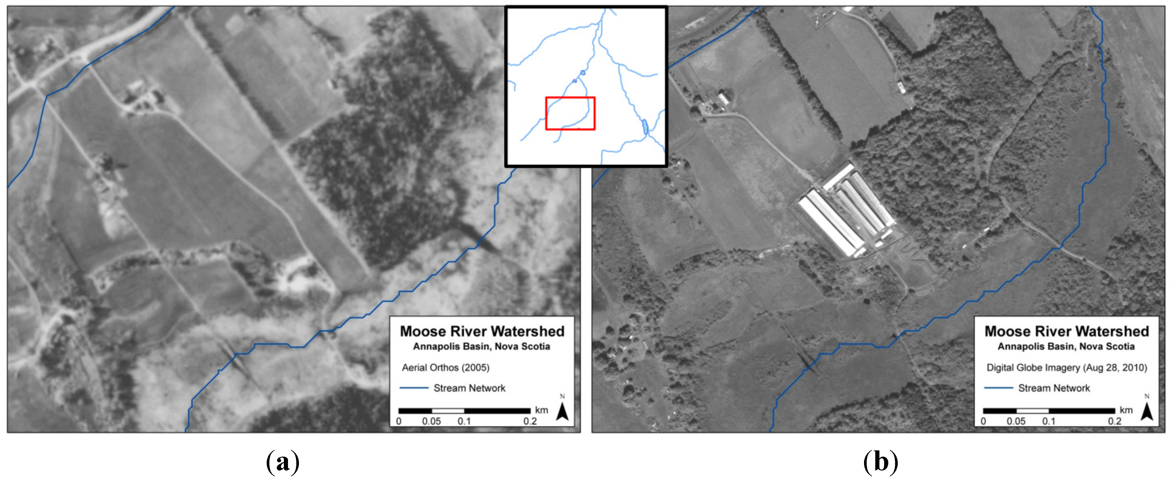
1
Applied Geomatics Research Group, Centre of Geographic Sciences (COGS), Nova Scotia Community College, 50 Elliot Road RR#1 Lawrencetown, Nova Scotia, NS B0S 1M0, Canada
2
Acadia Centre for Estuarine Research, Acadia University, 23 Westwood Avenue, Wolfville, Nova Scotia, NS B4P 2R6, Canada
3
Ivan Curry School of Engineering, Acadia University, Wolfville, Nova Scotia, NS B4P 2R6, Canada
*
Author to whom correspondence should be addressed.
Water 2014, 6(7), 1925-1944; https://doi.org/10.3390/w6071925
Submission received: 3 March 2014 / Revised: 2 June 2014 / Accepted: 20 June 2014 / Published: 4 July 2014

Abstract

:
The contamination of shellfish harvesting areas by fecal bacteria in the Annapolis Basin of Nova Scotia, Canada, is a recurring problem which has consequences for industry, government, and local communities. This study contributes to the development of an integrated water quality forecasting system to improve the efficiency and effectiveness of industry management. The proposed integrated forecasting framework is composed of a database containing contamination sources, hydrodynamics of the Annapolis Basin, Escherichia coli (E. coli) loadings and watershed hydrology scenarios, coupled with environmental conditions of the region (e.g., temperature, precipitation, evaporation, and ultraviolet light). For integration into this framework, this study presents a viable methodology for assessing the contribution of fecal bacteria originating from a watershed. The proposed methodology investigated the application of high resolution remote sensing, coupled with the commercially available product, MIKE 11, to monitor watershed land use and its impact on water quality. Remote sensing proved to be an extremely useful tool in the identification of sources of fecal bacteria contamination, as well as the detection of land use change over time. Validation of the MIKE 11 model produced very good agreement (R2 = 0.88, E = 0.85) between predicted and observed river flows, while model calibration of E. coli concentrations showed fair agreement (R2 = 0.51 and E = 0.38) between predicted and observed values. A proper evaluation of the MIKE 11 model was constrained due to limited water sampling. However, the model was very effective in predicting times of high contamination for use in the integrated forecasting framework, especially during substantial precipitation events.

1. Introduction

The contamination of shellfish harvesting areas by fecal bacteria in the Annapolis Basin, Nova Scotia, NS, Canada (Figure 1), is a recurring problem which has consequences for industry, government, and local communities. The proposed management system is the development of an integrated forecasting system to predict locations of Escherichia coli (E. coli) contamination. By knowing the spatial extent of poor water quality, regulation of bed closures will become more efficient and effective. The proposed integrated forecasting framework is composed of dynamic environmental conditions (e.g., temperature, precipitation, evapotranspiration, ultraviolet light), coupled with a database containing site-specific sources of contamination, watershed hydrology, estuarine hydrodynamics (MIKE 21), E. coli loadings scenarios and decay factors.
Figure 1. Annapolis Basin study area with Moose River catchment. Gauging station is located above tidal influence.
Water 06 01925 g001
For use in the integrated forecasting framework, the focus of this paper is to present a viable methodology for assessing the contribution of fecal bacteria contamination originating from a watershed. At present, industry regulators perform widespread closures of harvesting areas following heavy rainfall events. While wastewater treatment plants are considered the primary source of fecal contamination within the basin, the identification of other point and non-point sources from land use within the surrounding watersheds has been limited [1]. Regulators perform a survey of potential sources directly adjacent to the coast and do not examine potential sources higher in the watershed. As an alternate approach to industry regulation, this study investigates the use of high resolution remote sensing coupled with watershed modelling to monitor land use change and its impact on water quality.
In order for industry regulators to have a proper understanding of these sources of contamination and their effect on water quality, changes in land use need to be updated and assessed on a regular basis. Water quality monitoring is currently limited to the Annapolis Basin, therefore preventing the identification of unknown contaminant sources within the watersheds. The use of high resolution remote sensing presents a potential solution to this issue through its ability to efficiently locate and monitor changes in land use, enabling regulators to perform strategic water quality monitoring. This approach may offer improvements to targeted sampling protocols for many regulators facing budgetary constraints on field staff and water sampling.
Once sources of contamination are identified and evaluated, a modelling approach can be adopted to predict periods of high contamination. In this study we used a commercially available product, MIKE 11, to test the viability of this approach.
There is a substantial amount of past research into the modelling of water quality. However, the use of MIKE 11 to model fecal bacteria transport has been limited. Past applications of a river model such as MIKE 11 have been heavily focused on the design and operation of hydraulic structures, or for the purpose of flood prediction and analysis [2]. While little research has made use of MIKE 11 for the sole purpose of fecal bacteria modelling, other techniques and modelling methods have been used to estimate fecal bacteria loadings from watersheds, including time step limited models [3,4,5].
Valiela et al. [6] evaluated fecal coliform stock size and developed estimates of fecal bacteria loadings in Buttermilk Bay, Massachusetts. Sources of bacteria were identified and characterized, and the size of stocks was evaluated in sediment, the water column and sea wrack. Findings in this study suggested the re-suspension of fecal bacteria from sediment is a major contributor to high coliform levels in the water column. This introduces an important consideration to the modelling of fecal bacteria but was beyond the scope of our analysis and was not simulated in the study.
Riou et al. [7] investigated the contributions of fecal bacteria from small tributaries of a coastal area and their impact on shellfish quality. Their findings stressed the importance of the relationship between fecal pollution and high rainfall events. Following rainfall events and subsequent high flow conditions, fluxes in E. coli were 50 times higher than under normal weather conditions [7]. Kelsey et al. [8] developed a predictive model of bacterial contamination of shellfish using remote sensing precipitation data along with additional environmental and climatic data. The study findings indicated a substantial influence of temperature and salinity on bacteria concentrations. While these conditions were not investigated in this study, they will be further studied as part of the integrated water quality forecasting system.
The Soil and Water Assessment Tool (SWAT) microbial sub-model has been successfully applied to simulate the fate and transport of fecal bacteria on a daily time step [4,5,9]. Bougeard et al. [9] used the SWAT microbial sub-model to estimate E. coli fluxes in a catchment and its impact on the shellfish industry in Daoulas, France. This study stressed the importance of a continuous model to properly simulate constant fluxes of fecal bacteria from various sources. The advantage of continuous modelling in catchments and estuaries is the ability to assess response time and time of water quality recovery in realistic conditions [9].
Manache et al. [10] applied the continuous water quality model, DUFLOW, to simulate fecal bacteria concentrations in surface water. This study highlighted the importance of sufficient sampling for calibration and validation of models, which proved to be a limitation of this study. Liu et al. [11] modeled fecal coliform loadings in St. Louis Bay, Missouri using the Environmental Fluid Dynamic Code (EFDC) and Hydrological Simulation Program Fortran (HSPF). The EFDC was used to model the bay and major tributaries, while the HSPF was used to model the watersheds. Similar to Riou et al. [7], the study highlighted the influence of high flow conditions on fecal bacteria contamination. Two flow conditions—a dry weather and wet weather scenario—were modelled, with the latter exerting a greater stress on fecal coliform levels. Kelsey et al. [12] used Geographic Information Systems (GIS) and regression analysis to analyze relationships between land use and fecal coliform pollution in a South Carolina estuary. Fecal loadings from pets in urban areas were considered the primary source of pollution. More relevant to this study, the authors highlighted the importance of antecedent conditions on bacteria loadings, as they found a 48-hour rainfall total was more relevant to bacteria densities than a 24-hour total.
While the continuous simulations generated by the MIKE 11 model keep track of antecedent conditions, many other models explored were event-based models which do not have this capability. The ability of the MIKE 11 model to generate continuous simulations on an unlimited time step presented an advantage over time step limited models. For example, the SWAT model operates on a daily time step, and results in previous studies have drawn the conclusion that results are more favorable on a monthly temporal scale than a daily time frame [13]. The goal of the integrated forecasting system is to generate water quality forecasts, ideally within a 72-hour timeframe, so the ability of the model to run on an unlimited time step, along with its compatibility with the 2-dimensional estuarine model, MIKE 21, made it a practical model selection.

2. Materials and Methods
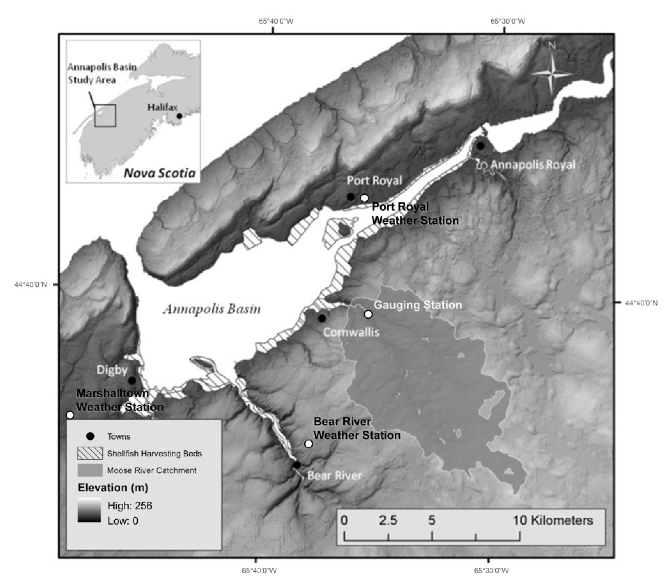
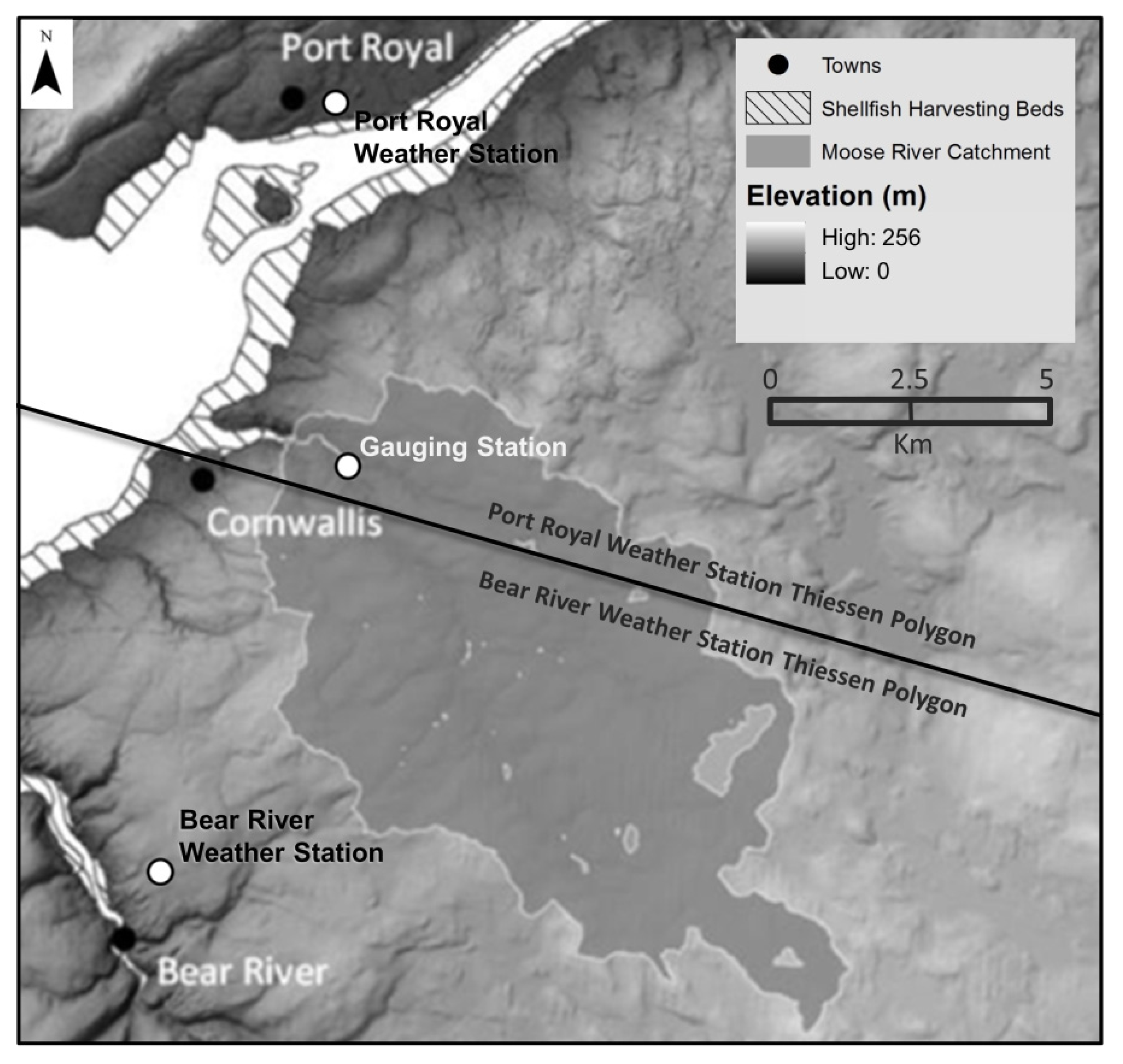
2.1. Study Area

The Annapolis Basin watersheds encompass an area with a wide variety of soil types, topography, and land cover. Six major rivers contributing to the Basin were gauged in late October of 2009. After monitoring these different rivers for water stage, flow, and fecal bacteria concentrations for approximately one year, the Moose River catchment was deemed the most appropriate study site to begin applying the MIKE 11 model.
The Moose River catchment is one of the largest contributors to the Annapolis Basin, encompassing an area of approximately 68 km2 (Figure 1). Of the six rivers monitored, the Moose River catchment consistently produced high levels of E. coli during high runoff events. This fact, along with the diverse soil types, topography and land cover, made Moose River a practical selection to evaluate the effectiveness of remote sensing and the MIKE 11 model in this study. The majority of the catchment is forested, accounting for approximately 66% of the land cover, followed by exposed soil (14%), agriculture (13%), wetlands and water bodies (6%), and developed areas (1%). Agricultural land cover in the area is dominated by hay fields, along with two mink farms that would later be considered a potential major contributor of fecal pollution. Soil types within the catchment have varying drainage characteristics, ranging from high clay content soils with poor drainage (low infiltration) to soils with excellent drainage (high infiltration). The topography of the region is varied, with average slopes of the river sub-catchments ranging from 3.2° to 11.8°. The average slope of the entire catchment is 6.5°.

2.2. MIKE 11 Model Description

The MIKE 11 model framework applied in this study is comprised of three major components: (1) the Rainfall Runoff (NAM) module; (2) the Hydrodynamic (HD) module; and (3) the Load Calculator and Advection Dispersion (AD) module. The NAM module simulates the volume of runoff produced for a given river catchment, which can then be routed along the river network using the hydrodynamic capabilities of the HD module. The GIS-based Load Calculator is then used to incorporate bacteria loadings to be transported through the river via the AD module. The MIKE 11 model has been successfully applied in several studies [2,14,15,16] for a variety of purposes, ranging from water resources planning, flood forecasting to water quality.
The NAM model was first developed at the Technical University of Denmark in the Institute of Hydrodynamics and Hydraulic Engineering [17]. NAM is the abbreviation of the Danish “Nedbør-Afstrømnings-Model”, meaning precipitation-runoff-model, also named RDII in English standing for Rainfall Dependent Inflow and Infiltration model. The NAM model is a lumped, conceptual model, which simulates rainfall runoff processes by continuously accounting for the water content in four storages: (1) snow storage; (2) surface storage; (3) lower (root zone) storage; and (4) groundwater storage [18]. Based on meteorological inputs of precipitation, potential evapotranspiration, and air temperature, the model generates catchment runoff split into overland flow, interflow and baseflow components.
The HD module is an implicit finite difference model for one-dimensional unsteady flow computation. Using the predicted runoff volumes from the NAM module, the HD module routes the water along the river network. Based on given boundary conditions, equations of conservation of continuity and momentum (Saint Venant equations) are solved numerically between the grid points for a given time interval [19].
The Load Calculator is used to determine the pollution loads of river catchments. Because the Load Calculator is incorporated into the ArcGIS interface, it has geographic capabilities of addressing the source location and subsequent transport of pollutants through river catchments. Incorporated as either point or non-point sources, pollutant loads are initially calculated as constant mass fluxes for each sub-catchment based on loading application rates and catchment runoff calculated in the NAM module [20].
Based on the resulting load calculation, the advection (i.e., transport) and dispersion of pollutants within waterways is simulated using the AD module, coupled with the hydrodynamics of the HD module. The AD module is based on the one-dimensional equation of conservation of mass of a dissolved or suspended material [21]. Once the hydrodynamics are modeled for a given river system, the HD module outputs of discharge, water level, cross sectional area and hydraulic radius is used in the advection dispersion equation. Like the HD module, this advection dispersion equation is solved using an implicit finite difference scheme.
In order to develop a simulation within the MIKE 11 model, several inputs and procedures are required to properly represent a natural system. In-field data collection, as well as post-processing of data, calibration and validation of simulations was involved in the modelling process.

2.3. Data Collection

2.3.1. River Stage and Discharge

A gauging station was established above tidal influence near the Moose River outlet in October 2009. An installed water level logger recorded water level readings at 15 minute intervals. Field visits to the site included water sampling and flow measurements, which involved the use of an electromagnetic velocity meter which measured the rate of flow. The geometry of the river bed (i.e., depth) and flow rates at the site of a cross section was measured at specific width intervals. From these measurements, the discharge of water (m3/s) could be calculated. As more flow measurements were collected, river discharge could be related to corresponding river stage readings through the development of a rating curve. The resulting time series of river discharge was then used for calibration and validation of the model.

2.3.2. Weather

Weather stations operated by the Applied Geomatics Research Group (AGRG) are located at three sites surrounding the Basin. Time series of rainfall were required for use in the NAM module to simulate the hydrology of the catchments, while a time series of air temperature was used for the calculation of potential evapotranspiration. Potential evapotranspiration accounts for all evaporation and plant transpiration within the watershed. Daily evapotranspiration values were calculated using the Penman-Monteith method [22]. This calculation requires daily mean air temperatures, wind speed, relative humidity, and solar radiation.
The Thiessen polygon method [23] was employed to determine the distribution of precipitation and temperature around the basin. The effect of altitude on temperature was assumed to be negligible, as most of the Moose River watershed is below 200 metres in elevation, with a maximum elevation of 220 m. Polygons were created by measuring the distance to the halfway point between two locations (i.e., weather stations), where a perpendicular bi-sector is created. Perpendicular lines were connected, forming a series of polygons with weather stations positioned in the centre of the polygons. If the catchment fell within a polygon, it was considered closer to that particular station than other stations. Referring to Figure 2, most of the Moose River catchment falls within the Bear River weather station Thiessen polygon, so meteorological data from this station was used as input into the MIKE 11 model.
Figure 2. Moose River catchment with Thiessen polygons. Bear River weather station meteorological data was used for input into the MIKE 11 model.
Water 06 01925 g002

2.3.3. Water Sampling and Lab Analyses

A total of 10 water samples were collected at the gauging station location in sterile bottles during the harvesting season for shellfish (April–November). These samples were used for the calibration of the model. Further samples were collected at targeted locations that were suspected sources of contamination. However, these samples did not contribute to the calibration of the model. The samples were 100 mL in volume, allowing for the determination of E. coli concentrations (Most Probable Number (MPN) 100 mL1) through lab analyses. Duplicate samples were collected to ensure validity of results. The IDEXX [24] Colilert Quanti-tray® system was used to enumerate bacteria in a collected water sample. A Colilert® reagent packet was added to each sample and shaken until dissolved.Samples were then transferred to IDEXX Quanti-trays® and sealed using a Quanti-tray® sealer.The trays were incubated at 37 °C for 22–24 h then counted using the MPN table provided by IDEXX. For a given 100 mL sample, a maximum number of bacteria could be enumerated (2420 MPN 100 mL1). For some sampling events, dilutions of samples were performed to address this limitation. This was accomplished through a procedure of adding an autoclaved volume of Milli-Q water to the water sample (e.g., 50 mL water sample +50 mL Milli-Q). Based on the number of times the sample was diluted, the number of fecal bacteria from the original sample could be calculated.

2.4. Model Requirements

2.4.1. Rainfall Runoff (NAM) Module

Development of the NAM module includes watershed delineation and calibration of the internal parameters. Watershed delineation was completed using RiverTools software with the use of a hybrid digital elevation model (DEM) of lidar (Light Detection and Ranging; collected and processed by AGRG) and a five-meter contour-derived DEM. For calibration of the internal parameters, the lumped catchment areas contributing to a gauging station were calculated for input into the NAM module. With the use of the created time series of rainfall and potential evapotranspiration, the NAM module was calibrated against observed values of discharge from 1 August to 31 December 2010.
The parameters of these models cannot, in general, be obtained directly from a measureable quantity of catchment characteristics [18]. However, in order to properly model the hydrodynamics of the river system, the entire watershed can be calibrated further at a more complex level (i.e., sub-catchments) by accounting for varied soil types, land cover and topography. To understand the distribution of hydrology efficiently, the use of the Soil Conservation Service (SCS) curve number (CN) method [25] and a gradient (slope) raster were implemented to develop a hydrologic measure of soil-land cover combinations and slope. It is important to note that there is no direct method of translating the calculated curve numbers and slopes into NAM parameters. Regardless, these calculations make it easier to understand the distribution of hydrology, and to reflect this distribution in the appropriate NAM parameters of the sub-catchments. Following this process, NAM parameters were adjusted accordingly using a trial and error process of calibration against observed values of discharge.

2.4.2. Hydrodynamic Module

The hydrodynamics of the river system require several data inputs, including the river network, cross sections, boundary conditions, channel roughness coefficients, and total runoff generated by the NAM module. The river network was created within RiverTools and edited within MIKE 11 GIS. Cross sections were created both digitally with the use of the DEM, and manually with collected survey data at various upstream and downstream locations of the river.
Boundary conditions are required by the model at upstream and downstream boundaries. For the upstream boundaries, the boundary applied can be assumed to equal a constant of zero (no discharge). This is because the NAM module is contributing water (overland flow, interflow and baseflow) to the river system via lateral inflow. Because the downstream boundary is located at the confluence of the river with the estuary, the boundary applied is a time series file of tidal water levels. These tidal water levels were extracted from MIKE 21 hydrodynamic simulations, previously generated for contribution to the integrated forecasting system. The channel roughness coefficient used in this study was the Manning (n) coefficient. The roughness coefficient is necessary to account for any flow resistance created by the river channel. This was calibrated against observed values of discharge for the period of 1 August to 31 December 2010.
The generated total runoff of the NAM module is divided into overland flow, interflow and baseflow components. Resulting time series of discharge can then be routed along the river network through a hydrodynamic simulation. Calibration of both the Manning coefficient and sub-catchment NAM parameters was then completed through a trial and error process.

2.4.3. Load Calculator and Advection Dispersion (AD) Module

Before using the Load Calculator and Advection Dispersion module, sources of fecal bacteria had to be identified and quantified in terms of potential loadings. The identification of bacteria sources were completed with the use of high resolution remote sensing, field and aerial surveys, available geographic data, and the review of appropriate literature. The major sources identified included agriculture, malfunctioning septic systems, waterfowl and other wildlife. Within the Load Calculator, pollutant loadings (i.e., concentrations) are calculated in the runoff of catchments by accounting for loading rates and runoff volume estimates from the NAM module. One challenge of the study was obtaining sufficient data concerning agriculture, as information regarding farming practices is considered confidential by agriculture regulators. In order to address this limitation, satellite imagery and aerial photography was used to identify the location of farm sites, and also proved to be effective in providing a better understanding of land use change over time. Unlike traditional Landsat satellite 30-metre pixel imagery, higher resolution imagery can provide details on land use and barn types in agricultural areas. For example, a large scale mink farm was identified within the Moose River catchment using 2010 Digital Globe World View 2 satellite imagery. However, the operation did not exist in 2005 according to an aerial photograph of the same location (Figure 3). This presented an efficient methodology in monitoring changes in land use and land cover over time. Once farm locations were identified, further information (e.g., livestock numbers) was gathered through correspondence with local farmers, while water sampling in adjacent waterways enabled the assessment of contamination risk.
Figure 3. Aerial photograph (2005) (a) and Digital Globe World View 2 satellite imagery (2010); (b) of mink farm site within Moose River watershed.
Water 06 01925 g003
A total of two large scale mink farm operations existed within the Moose River watershed. Unfortunately, no loading rates or bacteria concentration information could be found for mink species. Because this information was available for raccoon, it was assumed the diet and physiology of the two species was similar enough to apply the same loading rate. The loading rate applied was 3.71 × 10⁹ MPN∙day1 per individual [26].
A failure rate of 15% was applied to septic systems within the catchments, based on previous estimates of 10%–15% [27]. Failure rates of septic systems are site specific, as it is dependent on system type, soil type and maintenance frequency [28]. Septic loading rates were calculated according to the following equation:
L = RF × Q × C
  • L = Per capita loading rate (MPN person1∙day1);
  • RF = Failure rate (%);
  • Q = Per capita wastewater discharge (dL day1);
  • C = Wastewater E. coli concentration (MPN∙dL1).
The per capita wastewater discharge was assumed to be 70 US gallons (~265 L) per day [27]. The wastewater E. coli concentration was assumed to be 4.8 × 10⁶ MPN∙dL1 [28]. The resulting per capita loading rate (L) was 1.91 × 10⁹ MPN∙person1∙day1. Final household loading rates were calculated with the assumption that each home contains three people.
Population numbers of waterfowl and wildlife were gathered from 2 major sources—the Canadian Wildlife Service and the Department of Natural Resources, both of which conduct aerial and ground surveys of different species. Constant population densities, fecal bacteria concentrations [29] and loading rates (6.48 × 10⁷ MPN∙day1) [28] of waterfowl were applied to wetlands based on coverage areas. Population densities and loading rates [26] for raccoon (3.71 × 10⁹ MPN∙day1), beaver, muskrat and deer (1.6 × 10⁹ MPN∙day1) were applied to forested land based on coverage areas.
Runoff coefficients and decay rates are used within the Load Calculator to generate a more accurate measure of the loading that is available for transport via the advection dispersion module. In order to account for bacteria die-off from factors such as ultraviolet light and temperature, a distance decay rate was applied within the Load Calculator. Distance decay is a raster-based method of applying a first order decay rate of bacteria over a specified distance. As suggested by Walsh and Kunapo [30], a decay rate of 97% per 47 m was applied to septic system and agricultural loadings.
The runoff coefficient is a value indicating the amount of loading that is available for transport. Vinten et al. [31] suggested up to 14% of loadings applied by grazing sheep reached adjacent waterways. Fenlon et al. [32] suggested that 7% of E. coli loadings applied to grazing land was exported to field drain waterways during rainfall events. They also estimated that 2% of the exported load traveled below this field drain layer. In this study, mink farmers claimed that waste was contained and eventually removed from site. Upon further investigation, however, water samples taken both upstream (124 MPN∙mL1) and downstream (>2420 MPN∙mL1) of a farm site during a high rainfall event identified a potential source of E. coli contamination (Figure 4).
Further sampling during a separate rainfall event also yielded high counts downstream of the farm site (4840 MPN∙mL1). This created an obvious challenge in determining a practical runoff coefficient. After running simulations using various documented runoff coefficient values, a value of 5% applied to mink farm operations yielded the best agreement with observed counts of E. coli bacteria.
Figure 4. Water sample locations upstream and downstream of mink farm site (elevations represented by color—higher elevation: red/yellow; lower elevation: green/blue) (a); with corresponding total rainfall from Bear River weather station (b).
Water 06 01925 g004
The advection dispersion parameters include a dispersion coefficient (D), a dispersion factor (a), and the dispersion exponent (b). The dispersion coefficient is described as a function of the mean flow velocity (V) [21]:
D = a × Vb
The ability to calibrate AD parameters was limited for this study. Typical values of a dispersion coefficient range from 1–5 m2/s for small streams to 5–20 m2/s for rivers [21]. A dispersion factor of 20.0 and an exponent of 1.0 were selected for this study. It was assumed no substantial decay took place within the river, so no decay rate was applied within the advection dispersion module. Research on the decay of fecal bacteria is currently taking place for the purpose of this project, including the effect of ultraviolet light and temperature on decay rates. The results of this work will be applied within the model at a later date.

3. Results and Discussion

To properly evaluate the MIKE 11 model, two main statistical analysis methods were used: (1) the coefficient of determination (R2), and (2) the Nash-Sutcliffe Efficiency Index (E) [33]. These methods were applied to both the calibration (1 August–31 December 2010) and validation (1 April–31 July 2010) periods using a 15 min time step.

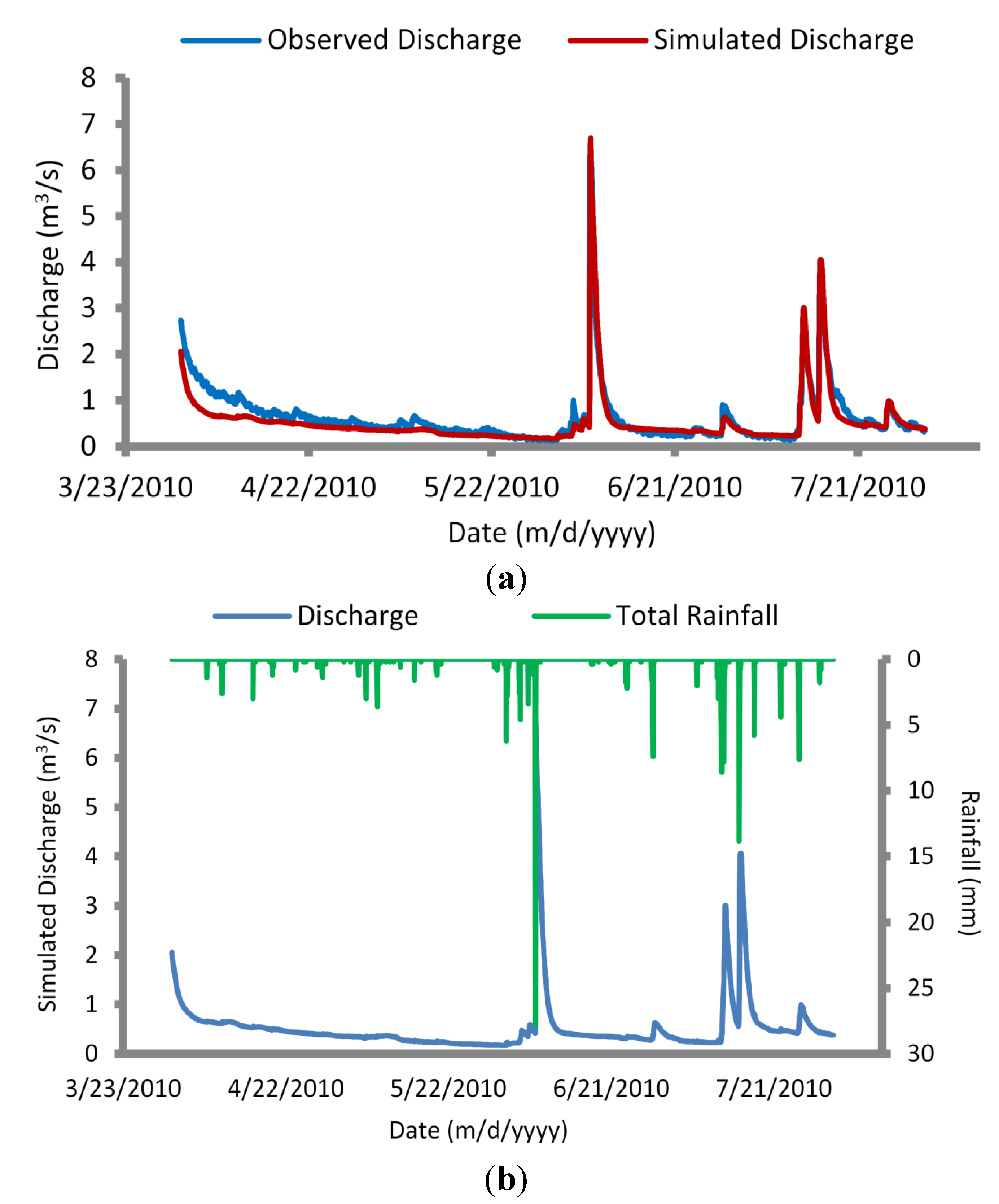
3.1. Rainfall Module

Final calibration of the lumped NAM parameters (Table 1) yielded R2 and E values of 0.93 and 0.91, respectively, indicating excellent agreement between simulated and observed discharge.
Table 1. Nedbør-Afstrømnings-Model (NAM) parameters of lumped Moose River catchment.
ParameterDescriptionParameter value
UmaxMaximum water content in surface storage (mm)13.0
LmaxMaximum water content in root zone storage (mm)100.0
CQOFOverland flow runoff coefficient (0–1)0.41
CKIFTime constant for routing interflow (hours)650
CK1,2Time constant for routing overland flow (hours)12
TOFRoot zone threshold value for overland flow (0–1)0.1
TIFRoot zone threshold value for interflow (0–1)0.1
TGRoot zone threshold value for groundwater recharge (0–1)0.1
CKBFTime constant for routing baseflow (hours)1000
These results are consistent with Jennings et al. [14] (R2 = 0.72–0.91), and superior to Shamsudin and Hashim [15] (E = 0.75), and were therefore considered sufficient for use in the HD module.

3.2. Hydrodynamic Module

Calibration of the HD module against measured flows yielded a Manning (n) roughness coefficient of 0.024. Adjusted NAM parameter values according to SCS curve number and slope distribution of the sub-catchments produced excellent correlation (R2 = 0.91) and very good agreement (E = 0.84) between predicted and observed flows for the calibration period.
The calibrated model was next simulated for a validation period of 1 April to 31 July 2010, producing very good agreement (R2 = 0.88 and E = 0.85) between simulated and observed flows (Figure 5). The mean observed discharge for the validation period was 0.63 m3/s, compared with a mean simulated discharge of 0.53 m3/s. The model captured peak discharge values within 1–4 h of observed flows. A 6 June 2010 rain event yielded observed flows of 6.4 m3/s, compared with simulated flows of 6.7 m3/s. Similarly, a 15 July 2010 rain event produced observed flows of 3.7 m3/s, compared with simulated flows of 4.1 m3/s. Assuming sufficient agreement of flows, calibration of the load calculator and advection dispersion parameters could be completed.
Figure 5. Simulated versus observed discharge values for validated hydrodynamic (HD) module (1 April–31 July 2010) (a); and observed rainfall versus simulated discharge values for validated HD module (b).
Water 06 01925 g005

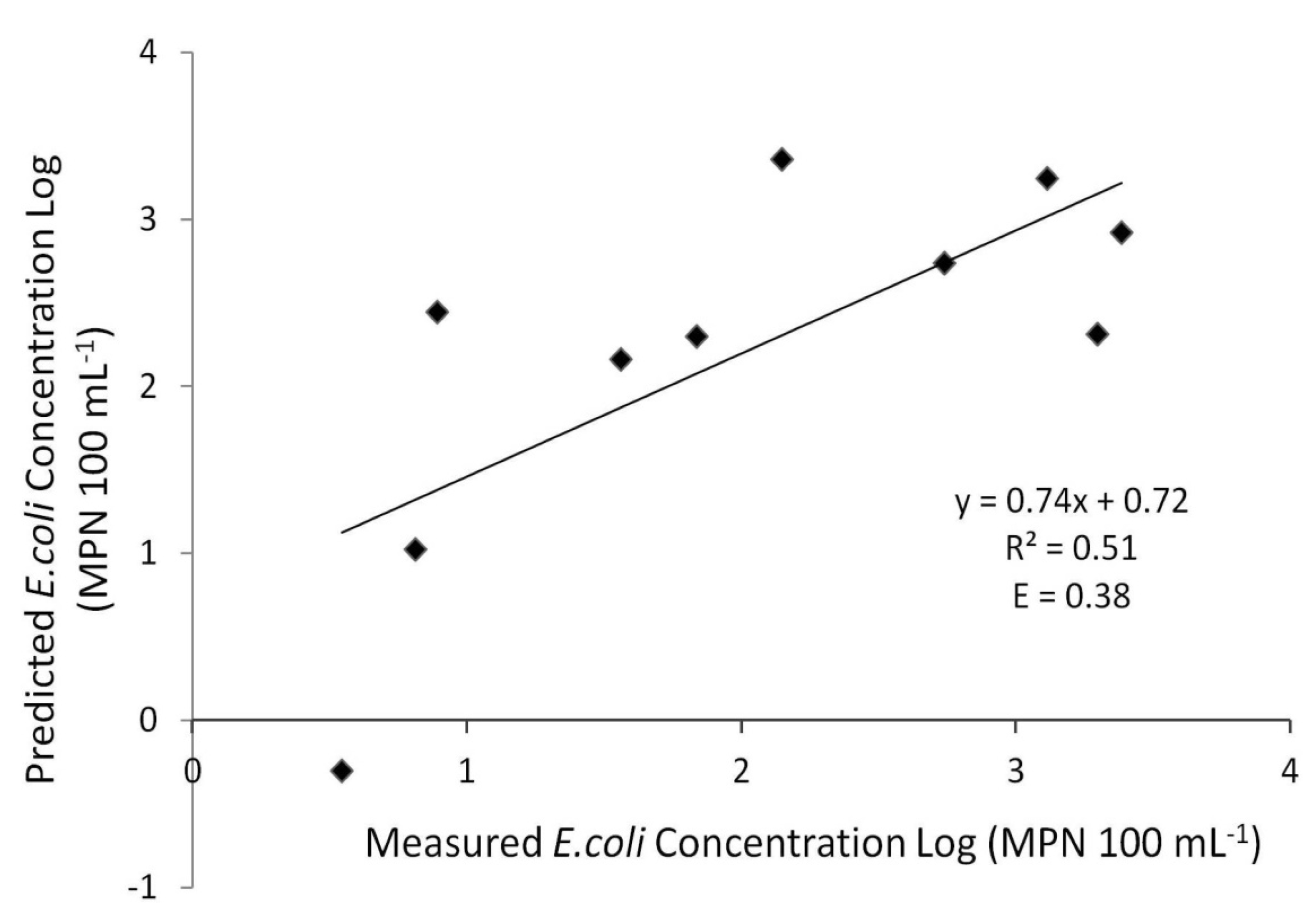
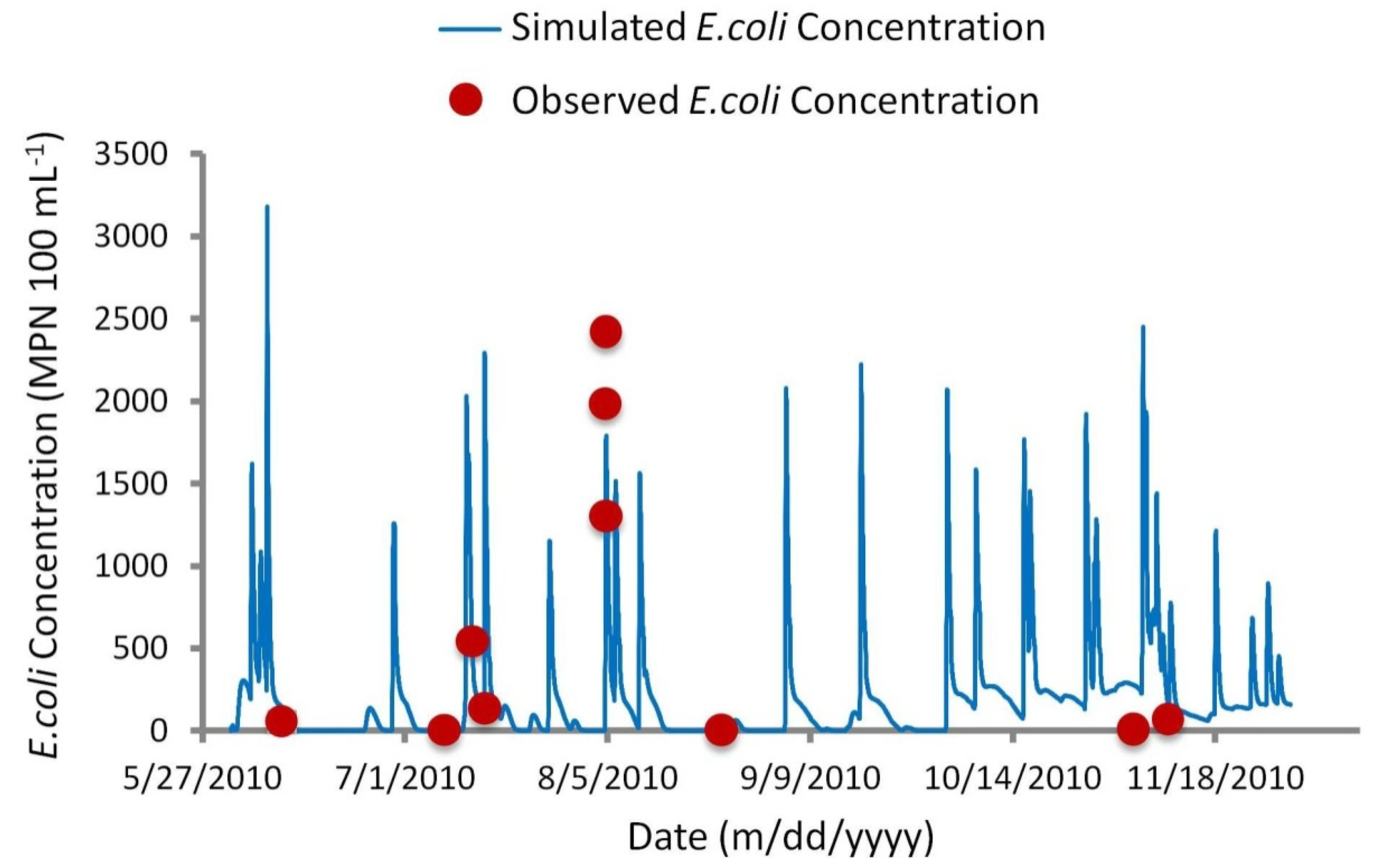
3.3. Load Calculator and Advection Dispersion Module
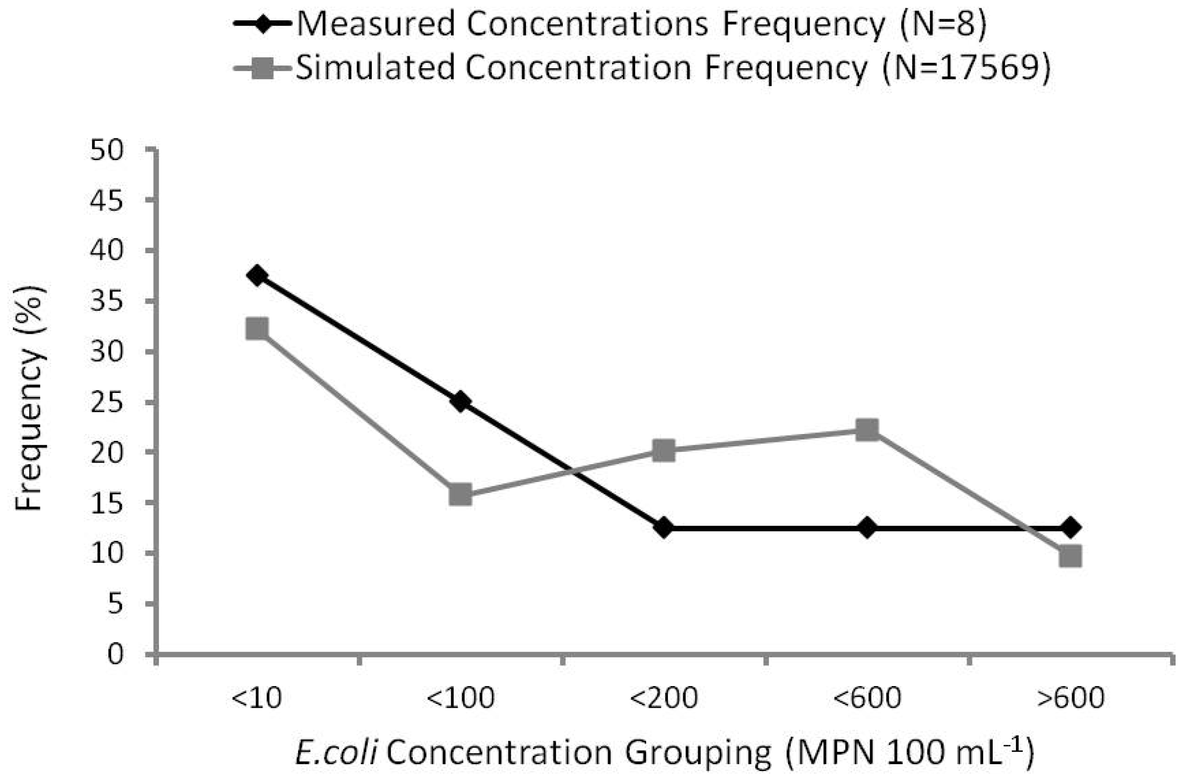
Insufficient sampling would not allow for both calibration and validation of the model. Calibration of the model was completed from June until November 2010 when water sampling took place. To normalize the bacteria concentration values, a log transformation was applied to evaluate the model performance. Following the log transformation, the calibrated model determined fair agreement (R2 = 0.51 and E = 0.38) between measured and predicted concentrations (Figure 6).
Model performance is comparable to results of Parajuli [13] (R2 = 0.36 and E = 0.21), who calibrated the SWAT model on a daily time step to model fecal bacteria. To address uncertainties in biological models, use of frequency curve analysis [4] and visual comparison [10,34] is recommended.
Frequency curve analysis compares observed and predicted frequency percentages. For example, 37.5% of measured E. coli concentrations were below 10 MPN 100 mL1, compared with 32.3% of simulated concentrations below the same concentration. Observed percentages were calculated based on a total sample number of eight water samples collected at the gauging station. Because three of the samples were collected during the same rain event (4 August 2010), it was considered one sample within one grouping (>600 MPN 100 mL1) to be more representative of the measured concentration frequency.
Figure 6. XY scatter of simulated versus observed E. coli concentrations (log transformed). Concentrations reflect bacteria concentrations at the study area gauging station.
Water 06 01925 g006
Analysis using this method produced fair correlation (R2 = 0.45) between simulated and observed concentrations (Figure 7). Baffaut and Benson [4] validated up to 70% of their frequency curve to compare model predicted concentrations with measured concentrations with average plus or minus one standard deviation. Bougeard et al. [9] obtained excellent agreement (R2 = 0.95 to 0.98) after applying frequency curve analysis.
Figure 7. Frequency curves (%) of simulated versus observed E. coli concentrations.
Water 06 01925 g007
The major requirement of the model for use in the water quality forecasting system is to identify periods of high contamination. As shown in Figure 7, frequency curve analysis has indicated the MIKE 11 model has achieved this requirement. Unfavorable results can be attributed to three major factors: (1) the small sample size of measured concentrations; (2) seasonal variability of loadings; and (3) the timing of discharge and concentration response.

3.3.1. Sample Size

The number of observed E. coli counts sampled was only ten for the advection dispersion calibration period of six months (Figure 8). Sampling began in June 2010 and continued on until November 2010. Sampling was not completed on a regular basis, and was heavily event-based during rain events.
Figure 8. Observed E. coli concentrations of Moose River water samples.
Water 06 01925 g008
Referring to Figure 9, visual comparison of observed versus simulated concentrations suggest more satisfactory agreement than the above statistical analysis implies. Small sample sizes make it very difficult to compute meaningful statistics as even one occurrence of poor agreement can distort an overall fit statistic [10]. For example, frequency analysis may address the issue of proper timing of simulations, yet a small sample size of measured values does not provide a sufficient representation of the physical or biological processes at work. As recommended by Canale et al. [34] and Manache et al. [10], a small sample size of measured concentrations often make statistical analysis redundant, leaving visual comparison as the only reliable method to evaluate a model.
Figure 9. Simulated versus observed E. coli concentrations for calibrated advection dispersion module.
Water 06 01925 g009

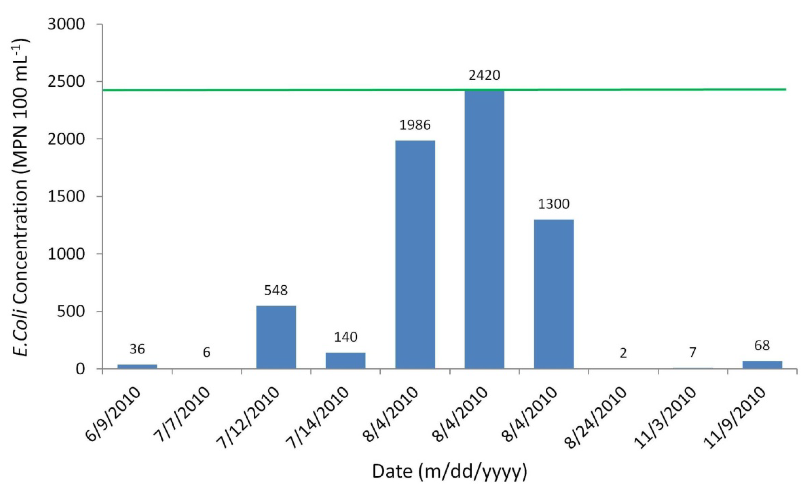
3.3.2. Seasonal Variation
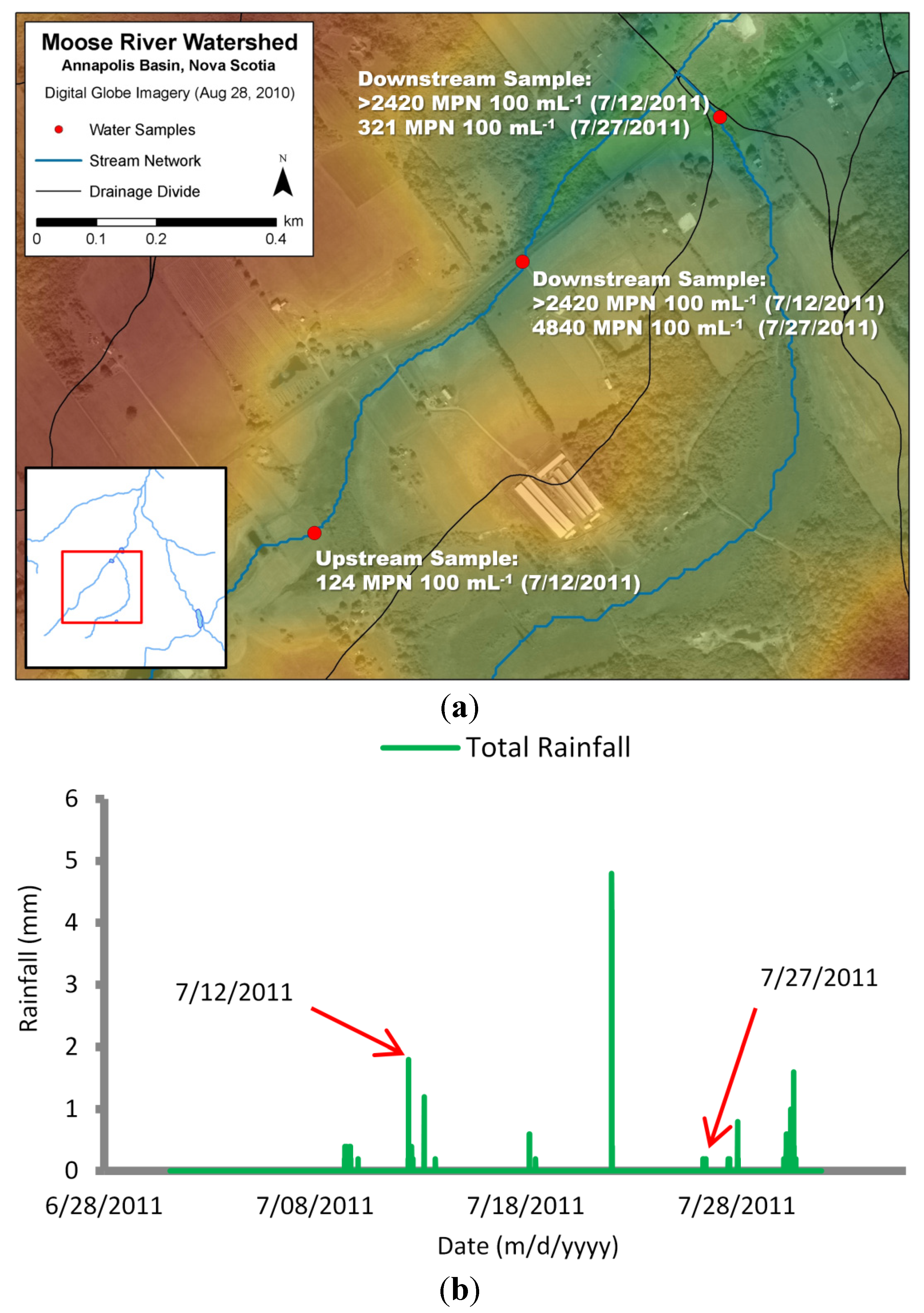
Seasonal variation in E. coli loadings can also be observed as reflected in the discharge and concentrations throughout the year. High simulated concentrations of E. coli are known to be heavily based on bacteria loadings from mink farms. Simulations run without mink farms yielded much lower peak concentrations (14 MPN 100 mL1) during the 4 August 2010 sampling event, compared with 1791 MPN 100 mL1 with mink farms included. Population numbers used were assumed to be at their highest—i.e., total number of mature males, females, and juvenile kits. This model did not address the dynamic process of the mink farming production cycle, which may explain disagreement between predicted and observed concentrations. For example, it is assumed the summer population of mink is at its peak following spring breeding and whelping. Over-estimation of concentrations during the November sampling (Figure 9) may suggest a decline in the mink population. Furthermore, information regarding the containment and fate of mink waste was limited. A correlation was observed between high rainfall events and high E. coli concentrations in waterways adjacent to the mink farms. During these rainfall events, it is possible the containment of waste was compromised. Additionally, information concerning possible spreading of mink waste on adjacent fields was not available, and was therefore not addressed in the model. The dynamic nature of farming presented a major challenge to this study. Local farm conditions are constantly changing, and are thus very difficult to model without firm knowledge of the farming process. While the use of remote sensing facilitates the identification of land use within an area of interest, this study exemplifies the importance of diligent field examination. Agriculture regulators consider information about farming practices confidential and do not make it available to the public domain. As a result, the availability of this information is heavily dependent on correspondence with farmers once new potential bacteria sources are identified.

3.3.3. Timing

While timing of concentrations during baseflow conditions is not an issue, prediction of the proper timing during high runoff events is more difficult. The model treats loadings as flow-based pollutants, so the timing of specific events is dependent on overland flow and interflow of the NAM module. For example, the model response to the 4 August 2010 rain event produced a quick increase in bacteria concentration, yet the response was approximately three hours later than measured values. Consequently, the model simulation for the 14 July 2010 rain event had the opposite response, generating a quick rise in concentration three hours earlier than measured values. Regardless of this, periods of high contamination were still captured in the model simulations, as indicated by the frequency curve analysis.

4. Conclusions

This study evaluated the use of high resolution remote sensing and watershed modelling to monitor fecal bacteria contamination resulting from land use practices. Remote sensing proved to be an extremely useful tool in the identification of sources of fecal bacteria contamination, as well as the detection of changes in land use over time. Water quality monitoring can present a challenge to water quality managers with limited budgets and human resources. The identification of these point and non-point sources through the use of remote sensing technologies will allow water quality managers to improve the efficiency and effectiveness of their monitoring programs through more focused water sampling and field examination.
This study has also shown that existing government data and current knowledge regarding the origin of fecal contamination has limitations in accurately predicting water quality. While the current focus of fecal contamination is attributed to municipal wastewater treatment plants, this study has indicated that other sources of contamination exist within a basin watershed. Furthermore, land use practices within a given area can be very dynamic, creating challenges in understanding their impact on water quality over time. This study presented a feasible alternative to industry regulation and water quality management involving the application of remote sensing to monitor these changes in land use, coupled with a watershed model to predict patterns of low and high E. coli contamination. While proper evaluation of the MIKE 11 model was constrained due to limited water sampling, the use of the model in producing a continuous estimation of E. coli, most notably during periods of high contamination, was shown to be promising for use in the integrated forecasting system.
Very favorable results were found for the calibration and validation of river flows, providing further support to the use of MIKE 11 as a valuable river modelling tool. The MIKE 11 model performed reasonably in predicting E. coli concentrations. However, for more comprehensive model assessment, there is a need for more sampling of water quality for the purpose of calibration and validation. A small sample number of measured concentrations made it difficult for proper evaluation of water quality prediction. However, considering this limitation, the model predictions of E. coli concentrations was very favorable. The main purpose of the model is to identify periods of high contamination. This study has shown that MIKE 11 is suitable for this purpose, as indicated by the frequency curve analysis.

Acknowledgments

The funding which enabled this study was provided by the Atlantic Innovation Fund (AIF) of the Atlantic Canada Opportunities Agency (ACOA). We would like to thank Mike Brylinsky of the Acadia Centre for Estuarine Research, Peter MacDermott and Shalon Oldford-MacLellan of the Applied Geomatics Research Group/Nova Scotia Community College (AGRG/NSCC), along with Greg Rose and Chris Inkratas of Golder Associates for their substantial contributions to this study. Thank you to David Colville and Wayne Reiger of AGRG/NSCC for providing the weather station data used in this study. Thank you to John Roos from Digital Globe for providing the World View 2 imagery. Thank you to Bruce Pollard of the Canadian Wildlife Service and Lawrence K. Benjamin of the Department of Natural Resources for supplying information on wildlife population surveys.

Author Contributions

Sean Butler was responsible for the data collection, model development, and subsequent analyses involved in this study. Tim Webster supervised the study, and provided guidance on all facets of this work, with particular focus on remote sensing, watershed modelling, and Geographic Information Systems (GIS). Anna Redden provided supervision through input on water quality and the research methodology applied in this study. Jennie Rand supervised this work through input on study design and water quality, and through her technical guidance with lab analyses. Nathan Crowell provided technical direction on remote sensing, GIS and watershed modelling, and made valuable contributions to the writing of this article. William Livingstone served as the project manager for this research, and provided guidance on the MIKE 11 model.

Conflicts of Interest

The authors declare no conflict of interest.

References

  1. Roberts, C.; Craig, C.; MacArthur, D.; Klaamas, P. Re-evaluation report of Nova Scotia Shellfish Growing Area NS-18-010-001—Annapolis Basin; EC Manuscript Report ST-AR-2009-04; Environment Canada: Dartmouth, Canada, 2009. [Google Scholar]
  2. Kamel, A.H. Application of a hydrodynamic MIKE 11 model for the Euphrates River in Iraq. Slovak J. Civ. Eng. 2008, 2, 1–7. [Google Scholar]
  3. Neitsch, S.L.; Arnold, J.G.; Kiniry, J.R.; Williams, J.R.; King, K.W. Soil and Water Assessment Tool Theoretical Documentation (version 2000); Grassland, Soil and Water Research Laboratory, Agricultural Research Service: Temple, TX, USA, 2002. [Google Scholar]
  4. Baffaut, C.; Benson, V.W. A bacteria TMDL for Shoal Creek using SWAT modelling and DNA source tracking. In Proceedings of the Total Maximum Daily Load (TMDL) Environmental Regulations–II of the Conference, Albuquerque, NM, USA, 8–12 November 2003; pp. 35–40.
  5. Parajuli, P.B.; Mankin, K.R.; Barnes, P.L. New methods in modelling source-specific bacteria at watershed scale using SWAT. In Proceedings of the Watershed Management to Meet Water Quality Standards and TMDLs (Total Maximum Daily Load) of the Conference, San Antonio, TX, USA, 10–14 March 2007.
  6. Valiela, I.; Alber, M.; LaMontagne, M. Fecal coliform loadings and stocks in Buttermilk Bay, Massachusetts, USA, and management implications. Environ. Manag. 1991, 15, 659–674. [Google Scholar] [CrossRef]
  7. Riou, P.; Le Saux, J.C.; Dumas, F.; Caprais, M.P.; Le Guyader, S.F.; Pommepuy, M. Microbial impact of small tributaries on water and shellfish quality in shallow coastal areas. Water Res. 2007, 41, 2774–2786. [Google Scholar] [CrossRef]
  8. Kelsey, R.H.; Scott, G.I.; Porter, D.E.; Siewicki, T.C.; Edwards, D.G. Improvements to shellfish harvest area closure decision making using GIS, remote sensing and predictive models. Estuaries Coasts 2010, 33, 712–722. [Google Scholar] [CrossRef]
  9. Bougeard, M.; Le Saux, J.C.; Pérenne, N.; Baffaut, C.; Robin, M.; Pommepuy, M. Modelling of Escherichia coli fluxes on a catchment and the impact on coastal water and shellfish quality. J. Am. Water Resour. Assoc. 2011, 47, 350–366. [Google Scholar] [CrossRef]
  10. Manache, G.; Melching, C.S.; Lanyon, R. Calibration of a continuous simulation fecal coliform model based on historical data analysis. J. Environ. Eng. 2007, 133, 681–691. [Google Scholar] [CrossRef]
  11. Liu, Z.; Hashim, N.B.; Kingery, W.L.; Huddleston, D.H. Fecal coliform modelling under two flow scenarios in St. Louis Bay of Mississippi. J. Environ. Sci. Health 2010, 45, 282–291. [Google Scholar] [CrossRef]
  12. Kelsey, H.; Porter, D.E.; Scott, G.; Neet, M.; White, D. Using geographic information systems and regression analysis to evaluate relationships between land use and fecal coliform bacterial pollution. J. Exp. Mar. Biol. Ecol. 2004, 298, 197–209. [Google Scholar] [CrossRef]
  13. Parajuli, P.B. SWAT Bacteria Sub-model Evaluation and Application. Ph.D. Thesis, Kansas State University, Manhattan, NY, USA, 2007. [Google Scholar]
  14. Jennings, S.; Elsaesser, B.; Baker, G.; Bree, T.; Daly, D.; Fitzpatrick, J.; Glasgow, G.; Hunter-Williams, T. An Integrated Approach to Quantifying Groundwater and Surface Water Contributions of Stream Flow; RPS Consulting Engineers Ltd.: Belfast, Northern Ireland, UK, 2000. [Google Scholar]
  15. Shamsudin, S.; Hashim, N. Rainfall runoff simulation using MIKE 11 NAM. J. Civ. Eng. 2002, 15, 1–13. [Google Scholar]
  16. Malakahmad, A.; Eisakhani, M.; Isa, M.H. Developing MIKE-11 model for water quality simulation in Bertam River, Cameron Highlands. National Energy University, Kuala Lumpur, Malaysia, 16–20 June 2008.
  17. Nielsen, S.A.; Hansen, E. Numerical simulation of the rainfall runoff process on a daily basis. Nord. Hydrol. 1973, 4, 171–190. [Google Scholar]
  18. Madsen, H. Automatic calibration of a conceptual rainfall-runoff model using multiple objectives. J. Hydrol. 2000, 235, 276–288. [Google Scholar] [CrossRef]
  19. Texas A&M. Texas A&M University and U.S. Bureau of Reclamation Hydrologic Modelling Inventory, Model Description Form, MIKE 11; Texas A&M University: College Station, TX, USA, 1999. [Google Scholar]
  20. Danish Hydraulic Institute. MIKE 11 GIS User’s Guide; DHI: Hørsholm, Denmark, 2009. [Google Scholar]
  21. Danish Hydraulic Institute. MIKE 11 Reference Manual; DHI: Hørsholm, Denmark, 2011. [Google Scholar]
  22. Neitsch, S.L.; Arnold, J.G.; Kiniry, J.R.; Williams, J.R. Soil and Water Assessment Tool Theoretical Documentation (version 2005); Grassland, Soil and Water Research Laboratory, Agricultural Research Service: Temple, TX, USA, 2005. [Google Scholar]
  23. Thiessen, A.H. Precipitation averages for large areas. Mon. Weather Rev. 1911, 39, 1082–1089. [Google Scholar]
  24. Colilert. Available online: http://www.idexx.com/view/xhtml/en_us/water/colilert.jsf?conversationId=55424 (accessed on 25 October 2010).
  25. U.S. Soil Conservation Society. Section 4 Hydrology. In National Engineering Handbook; U.S. Department of Agriculture, Soil Conservation Service: Washington, DC, USA, 1956. [Google Scholar]
  26. MapTech Inc. Fecal Coliform TMDL (Total Maximum Daily Load) Development for Upper Blackwater River, Virginia; Virginia Department of Environmental Quality and Virginia Department of Conservation and Recreation: Blacksburg, VA, USA, 2000. [Google Scholar]
  27. U.S. Environmental Protection Agency. nsite Wastewater Treatment System Manual; EPA-625-R-00-009; U.S. Environmental Protection Agency: Washington, DC, USA, 2002. [Google Scholar]
  28. Petersen, C.M.; Rifai, H.S.; Stein, R. Bacteria load estimator spreadsheet tool for modelling spatial Escherichia coli loads to an urban bayou. J. Environ. Eng. 2009, 135, 203–217. [Google Scholar] [CrossRef]
  29. Alderisio, K.A.; DeLuca, N. Seasonal enumeration of fecal coliform bacteria from the feces of ring-billed gulls (Larus delawarensis) and Canada geese (Branta canadensis). Appl. Environ. Microbiol. 1999, 65, 5628–5630. [Google Scholar]
  30. Walsh, C.J.; Kunapo, J. The importance of upland flow paths in determining urban effects on stream ecosystems. J. N. Am. Benthol. Soc. 2009, 28, 977–990. [Google Scholar] [CrossRef]
  31. Vinten, A.J.A.; Douglas, J.T.; Lewis, D.R.; Aitken, M.N.; Fenlon, D.R. Relative risk of surface water pollution by E. coli derived from faeces of grazing animals compared to slurry application. Soil Use Manag. 2004, 20, 13–22. [Google Scholar] [CrossRef]
  32. Fenlon, D.R.; Ogden, I.D.; Vinten, A.; Svoboda, I. The fate of Escherichia coli and E. coli O157 in cattle slurry after application to land. J. Appl. Microbiol. 2000, 88, 149–156. [Google Scholar] [CrossRef]
  33. Nash, J.E.; Sutcliffe, J.V. River flow forecasting through conceptual models part I—A discussion of principles. J. Hydrol. 1970, 10, 282–290. [Google Scholar] [CrossRef]
  34. Canale, R.P.; Auer, M.T.; Owens, E.M.; Heidtke, T.M.; Effler, S.W. Modelling fecal coliform bacteria–II. Model development and application. Water Res. 1993, 27, 703–714. [Google Scholar] [CrossRef]

