Flow Forecasting using Deterministic Updating of Water Levels in Distributed Hydrodynamic Urban Drainage Models

Abstract

There is a growing requirement to generate more precise model simulations and forecasts of flows in urban drainage systems in both offline and online situations. Data assimilation tools are hence needed to make it possible to include system measurements in distributed, physically-based urban drainage models and reduce a number of unavoidable discrepancies between the model and reality. The latter can be achieved partly by inserting measured water levels from the sewer system into the model. This article describes how deterministic updating of model states in this manner affects a simulation, and then evaluates and documents the performance of this particular updating procedure for flow forecasting. A hypothetical case study and synthetic observations are used to illustrate how the Update method works and affects downstream nodes. A real case study in a 544 ha urban catchment furthermore shows that it is possible to improve the 20-min forecast of water levels in an updated node and the three-hour forecast of flow through a downstream node, compared to simulations without updating. Deterministic water level updating produces better forecasts when implemented in large networks with slow flow dynamics and with measurements from upstream basins that contribute significantly to the flow at the forecast location.

1. Introduction

The increasing richness of hydrological data from cities leads to an increasing use of spatially distributed continuous hydrologic simulation models [1]. Another driver for this development will be the need for online versions of models referred to as “models of everywhere” [2]: models even providing predictions for ungauged parts of the system. Recent examples of such models can be found in studies discussed by [3,4]. In the latter example, a distributed hydrodynamic urban runoff model with a water quality module is used to model the concentrations of pollutants and pathogens in urban floodwater for the city of Dhaka, Bangladesh. An online version of such a model could be used to give precise and proper warnings about the health risks involved in being exposed to flood water, as well as forecasting the hydraulic load on a downstream wastewater treatment plant.

For any online model that is used for real-time decision-making it is crucial to keep the model in touch with reality, e.g., by assimilating measurements into the model. For simple, linear models this can be achieved using a version of the Kalman Filter [5]; recent examples, using a lumped conceptual urban runoff model and an Extended Kalman filter, are provided by [6,7]. For large or very non-linear models ensemble-based data assimilation methods, such as the Ensemble Kalman Filter [8,9] or the Particle Filter [10,11], would usually be required to obtain satisfactory results. These methods require large ensembles of model runs, for which reason the models have to be rather fast for the updating scheme to work in real-time applications. The commercially available physically based, distributed, hydrodynamic urban drainage models such as SWMM (US EPA, NW, Washington, DC, USA) [12], MIKE URBAN (DHI, Hørsholm, Denmark) [13], and InfoWorks CS (Innovyze, Broomfield, CO, USA) [14] are, however, neither simple nor fast. Even though their description of surface runoff processes is lumped-conceptual at the sub-catchment scale and computationally fast, the distributed-physical part describing the hydrodynamics of pipe flows solves partial differential equations that are computationally more demanding. For instance, a physically based, distributed urban drainage model was recently developed for a part of the drainage system of Copenhagen (Denmark) that discharge wastewater from more than half a million people to the Lynetten wastewater treatment plant. The model covers an area of 76 km² and includes 5000 nodes [15]. Even though the model mainly includes the largest pipes and most important detention basins and overflow structures (corresponding to about 20% of the nodes in the real pipe system), it runs rather slowly - in close to real time on powerful desktop computers available by the year 2013 [16]. Therefore, ensemble based assimilation methods and forecast runs are currently computationally unfeasible. Filtering data assimilation methods based on a steady Kalman gain have been applied with success for computationally burdensome distributed river models [17], but this method requires that the distribution of the model error can be assumed constant in time, which is not a reasonable assumption for an urban drainage model [18]. The branched nature of urban drainage systems with a mixture of fast and slow response times and large differences in local gradients makes successful implementation of classical data assimilation tools in distributed hydrodynamic urban drainage models complicated and very computationally expensive.

Perhaps due to the limitations mentioned above there are no references in the open literature to applications of data assimilation methods applied to the hydrodynamic part of distributed urban drainage models. The only available data assimilation tool for this kind of model that the authors have come across is MOUSE UPDATE; a pragmatic tool that inserts measured water levels or flows directly into the hydrodynamic module of the MIKE URBAN software. This alternative updating method (in the following referred to as “deterministic updating”, or the “Update” method) ensures that the simulations are in accordance with the available measurements, and it should thereby result in an improvement in model forecasting performance. The Update method has been used in a few practical urban drainage projects, but their results are not publically accessible. The authors have presented initial studies of the Update method in conference contributions [19,20] but this paper is the first to present and document the performance of this deterministic updating method in the open literature. The work focuses on water level updating for increasing flow forecasting performance, as water levels are the most widespread type of measurements available in urban drainage systems.

The article is divided into six sections: 1: Introduction; 2: Update Procedure; 3: Evaluation Procedure; 4: Case Studies; 5: Discussion; and 6: Conclusions. Section 2 presents the theory behind the updating procedure along with a short description of how to use the tool, and Section 3 describes how the efficiency of the update is evaluated in this article. Section 4 is divided into two parts. First a hypothetical example is presented, which illustrates how Updating can make use of level measurements with a limited range, how it can compensate for an inflow to the system that is not accounted for by the model or the applied boundary conditions and that the water balance of the model fits when updating is active. Then the update procedure is tested on a real model implementation for the city of Kolding (Denmark). Here the model is updated using water level measurements from eight different locations, and the resulting simulated outflow is compared with both the measured outflow and the outflow simulated without updating. The results also include a presentation of the increased forecast potential using updating. Section 5 discusses the catchment features that affect the updating performance and section 6 draws conclusions on the general applicability of the investigated Update method.

2. Update Procedure

2.1. Overall Structure of the MIKE URBAN Model

Physically based, distributed hydrodynamic urban drainage models, such as the MIKE URBAN model, are the most detailed type of models available for urban drainage systems. They are divided into two main components: a surface module and a hydrodynamic model. The surface module converts precipitation data into inflow to the pipe system for each sub-catchment in the system, while the hydrodynamic model calculates the flow in the pipe system using the flow from the surface module as model forcing. Additional model forcing components can furthermore be defined, such as infiltration-inflow or pumped flows. The surface module is lumped-conceptual on the sub-catchment scale but since these are distributed in space the surface module itself can be regarded as a distributed model. Several types of surface modules are available; the one used here is based on a time-area principle. The hydrodynamic model is physically distributed and like for the surface module several version are also available; the one used here is the MOUSE hydrodynamic engine.

There are several examples in the literature of updating the lumped-conceptual part of MOUSE models. In [21] a MOUSE model is e.g., auto-calibrated for a 0.8 km² suburban catchment at 30 min time-intervals by adjusting an overall system scaling factor, the surface concentration time and the dry weather flow, and in [22] the lumped-conceptual hydrological states of the Rainfall Dependent Infiltration and Inflow module (RDII) are updated (DHI, 2009). This is however fundamentally different from updating the states of the hydrodynamic part of the model, as done in this paper.

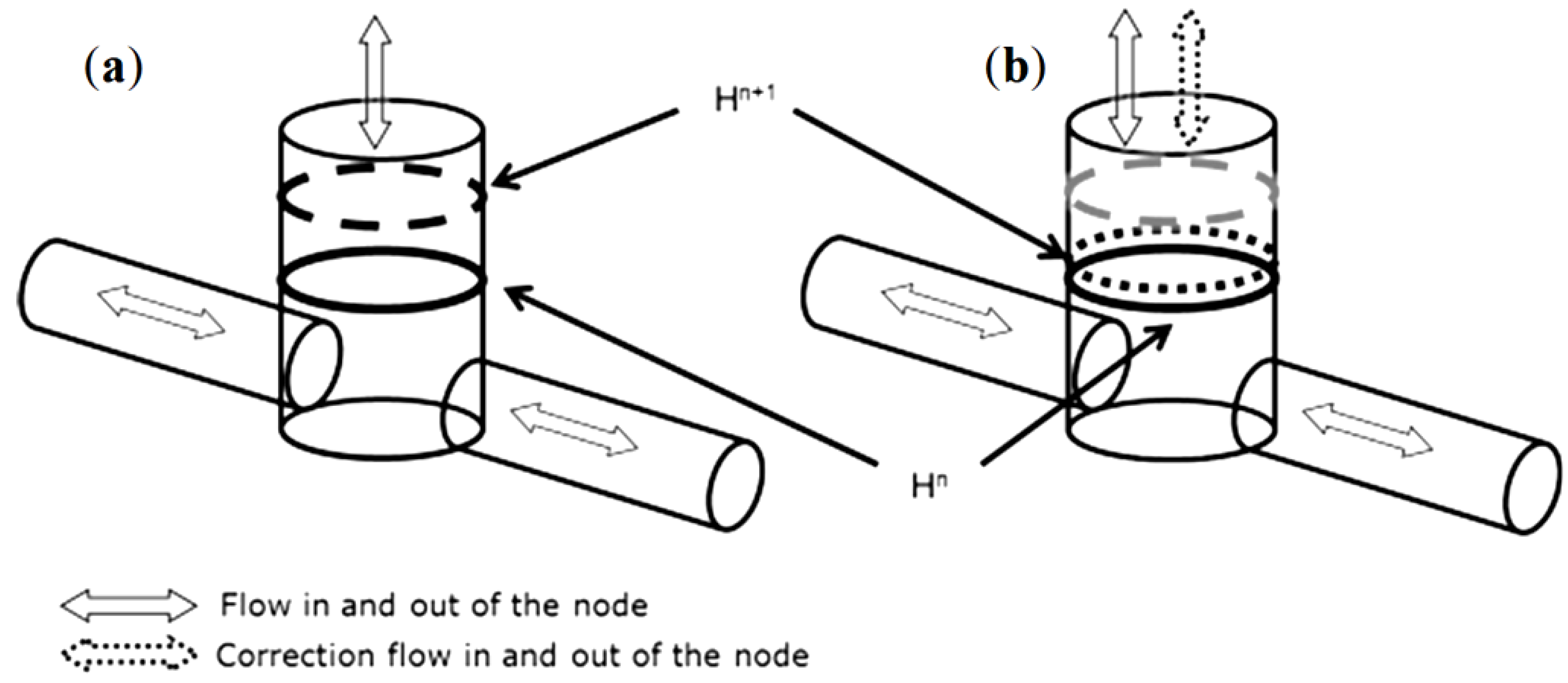
2.2. Theoretical Basis for the Update Procedure

The computation technique applied in the MOUSE hydrodynamic (HD) engine for solving the Saint Venant Equations uses a double sweep algorithm, which solves two sets of equations that are set up using a “branch” and a “nodal” matrix [23,24]. In short, the “branch” matrix is applied for computing flows and water levels in the pipes as a function of the water levels in the nodes at the end of each pipe, whereas the “nodal” matrix is used for computing water levels in the nodes at the new time step. Equation (1) gives the finite difference approximation of the continuity equation for a node:

(1)

where the terms of the equation are: the sum of inflows (q_in) and outflows (q_out); the time step (Δt); the water level (H); the wetted cross-section area (A_cr); the current and next time steps (n and n+1) and the intermediate time steps (n−½ and n+½). Figure 1a illustrates how the water level at the next time step (Hⁿ⁺¹) is estimated.

Figure 1. Normal (a) HD node computation and (b) Update node computation. In this example, the correction flow extracts the volume of water necessary to lower the water level from the level corresponding to the dashed circle to the level corresponding to the dotted circle.

Figure 1. Normal (a) HD node computation and (b) Update node computation. In this example, the correction flow extracts the volume of water necessary to lower the water level from the level corresponding to the dashed circle to the level corresponding to the dotted circle.

The idea behind the Update procedure is that the new water level in the node is known from a measurement produced by a level sensor located in the node. This means that the so far unknown variable in Equation (1), Hⁿ⁺¹, is now given by data taken from a measurement. A new unknown variable, Q_correction, is then introduced on the right-hand side of Equation (1):

(2)

Figure 1 illustrates the difference between Equations (1) and (2). In the figure to the left Hⁿ⁺¹ is illustrated by the dashed circle, while in the figure to right it is illustrated by the dotted circle, which equals the measured water level. The difference between the simulated water level without updating and the updated water level (which is equal to the measured level) is the result of updating with the correction flow, Q_correction. This correction can generally either add or extract water, which is illustrated by the dotted vertical double arrow in Figure 1b, but in the example shown it extracts water as evidenced by a lowering of Hⁿ⁺¹ compared with Figure 1a. The deterministic updating method is computationally efficient compared with updating schemes using the classical filtering techniques mentioned in the introduction, because corrections to the simulation are done only at the point where the level sensor is located and because distribution of the correction flow is ensured by the ordinary HD computations.

A similar method has been implemented for the use of measured flow data for updating in computational grid points in the pipes where flow gauges are located. To make the computation match the measured flow, a correction flow is introduced that adds or extracts water from the pipe at the location of the flow gauge. In this case, another set of equations is rearranged to make the update computation, but the basic principle is the same as in the water level updating procedure described above.

When using a model in real time, measured data can only be available until the present time t from whereon any further simulation creates a forecast. It is possible to compute the update correction flow as described above only as long as measured values are available (up to time t). From this point in time, updating (Equation (2)) is switched off and the continuity equation is solved in the standard way (Equation (1)).

2.3. Water Balance

The flow added or extracted in the computation in order to make the resulting water level match the measured water level is fully reported to the results as a correction flow time series and as the accumulated volume of the correction flow, together with a logging of the periods where the update function has been active. This means that updating does not ruin or violate the water balance of the simulation.

2.4. Controlling the Update Procedure

The updating feature can be configured to work only when the applied sensor signal is within a specified range. This is relevant when using sensors with known maximum or minimum limits. Pressure-based water level gauges can, for instance, only measure levels that are above the level of the sensor, while an ultrasonic water level gauge only measures correctly when the water level is below the sensor.

An adjustment factor that is multiplied with the calculated correction flow before this enters the model can furthermore be specified for each location where the update feature is applied. This is useful in situations with noisy measurements or when big and sudden corrections are prone to create problems for the model. An adjustment factor less than one will make the corrections smoother and thus limit the risk of introducing large gradients between the state value in the updated node and its neighbors; however, it will also make updating react slower. Since the purpose of the presented work has been to study the maximum effect of the update feature, the adjustment factor is set to one in all examples presented in the paper.

3. Evaluation Procedure

3.1. Downstream Flow Evaluation

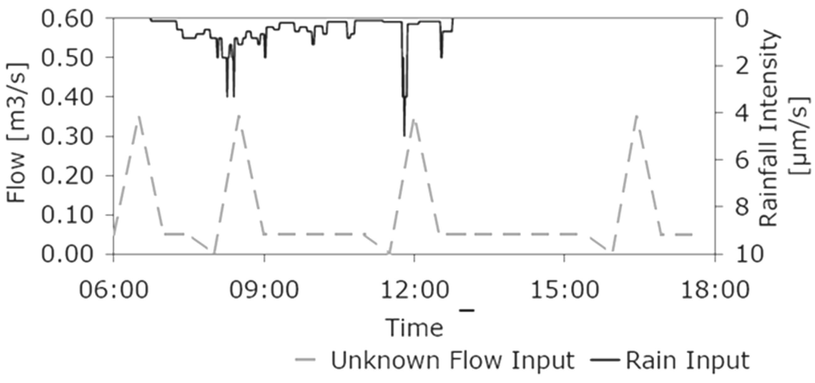
When a model’s upstream water levels are updated to more true-to-life values, the impact will propagate with the flow down through the system, in which case downstream flow simulations are likely to improve as well, given that the behavior of the physical system is described correctly by the model. In the following examples, water levels are updated in one or several nodes at a time. The effect of each update is examined by comparing measured downstream flows with the corresponding flows simulated with and without updating in upstream nodes. The forecast potential from updating is also examined. This is achieved by comparing the simulation results t_f minutes after updating has ceased with the simulation results from a model run completely without updating.

3.2. Rainfall Input

Good rainfall forecasts up to a few hours into the future (nowcasts) are likely to become available within the next few years as a result of utilizing improvements within radar forecasting in combination with numerical weather prediction models [25,26,27,28,29]. A major assumption in our work, however, is that future rainfall input is known during all simulations, i.e., we use measured rainfall (“perfect forecasts”) as a surrogate for rainfall forecast time series. Besides being convenient from a computational point of view, this also has the benefit of isolating the impact of the update from errors related to rainfall forecasting.

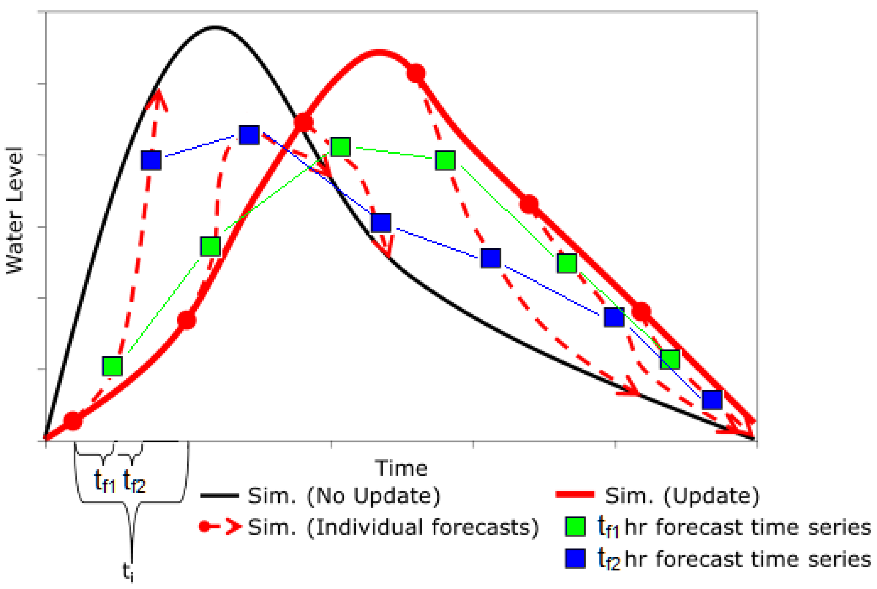
3.3. Generating Forecast Time Series for Testing the Algorithm

The t_f minute forecasts shown in the paper are made by assimilating water levels in one or more nodes until time t, at which point updating is turned off and the simulation continues without updating until the time when the forecast is required (t + t_f), as shown in Figure 2 for two different forecast time horizons (t_f1 and t_f2).

After updating stops, the change to state variables incurred by the updating algorithm will gradually loose its importance and the simulated values will converge towards the simulation run without updating, as illustrated by the dashed lines on Figure 2. To generate, for example, a 60-min forecast (t_f = 60 min) the HD model is run with updating until time t, and thereafter it is run without updating for another 60 min until time t + 60 min. The result after 60 min is then part of the 60-min forecast time series. To make a 60-min forecast time series with a temporal resolution (t_i) of 2 min the forecast states at 2 min intervals (generated with updating) are used to initialize the 60-min forecasts, i.e., the computer workload increases by a factor of 30 compared to a single model run in the same period. In this work, a 10-min temporal resolution is used when generating the forecast time series, in order to keep the computational burden at an acceptable level.

Figure 2. Sketch of how the forecasting time series is produced. The black and red solid curves represent simulation results when the model is run without and with updating, respectively. The dashed curves represent simulation results from a model run with updating (red solid curve) until the dot, after which the simulation continues without updating. The time between these dots (t_i) is the time step of the forecast time series, and the squares connected with thin lines represent points in the t_f hour forecast time series. Two examples of forecast time series are shown, for a short (t_f1, green squares) and a long (t_f2, blue squares) forecast horizon.

Figure 2. Sketch of how the forecasting time series is produced. The black and red solid curves represent simulation results when the model is run without and with updating, respectively. The dashed curves represent simulation results from a model run with updating (red solid curve) until the dot, after which the simulation continues without updating. The time between these dots (t_i) is the time step of the forecast time series, and the squares connected with thin lines represent points in the t_f hour forecast time series. Two examples of forecast time series are shown, for a short (t_f1, green squares) and a long (t_f2, blue squares) forecast horizon.

The process of generating the forecast time series for the purpose of testing the Update algorithm, as illustrated in Figure 2, is automated in our work by using a Visual Basic program that runs all the forecast simulations, extracts the required results and then adds them to the forecast time series. The workflow’s first step is to produce model states for the updated model for the time steps that are going to be used as offset for each forecast. This is done by running a single simulation with updating enabled for the entire period of interest. The state values from this simulation for all relevant time steps are saved to a single “hotstart” result file, which is used to initialize the model before each forecast simulation. During forecast simulations, updating is disabled.

4. Application Examples

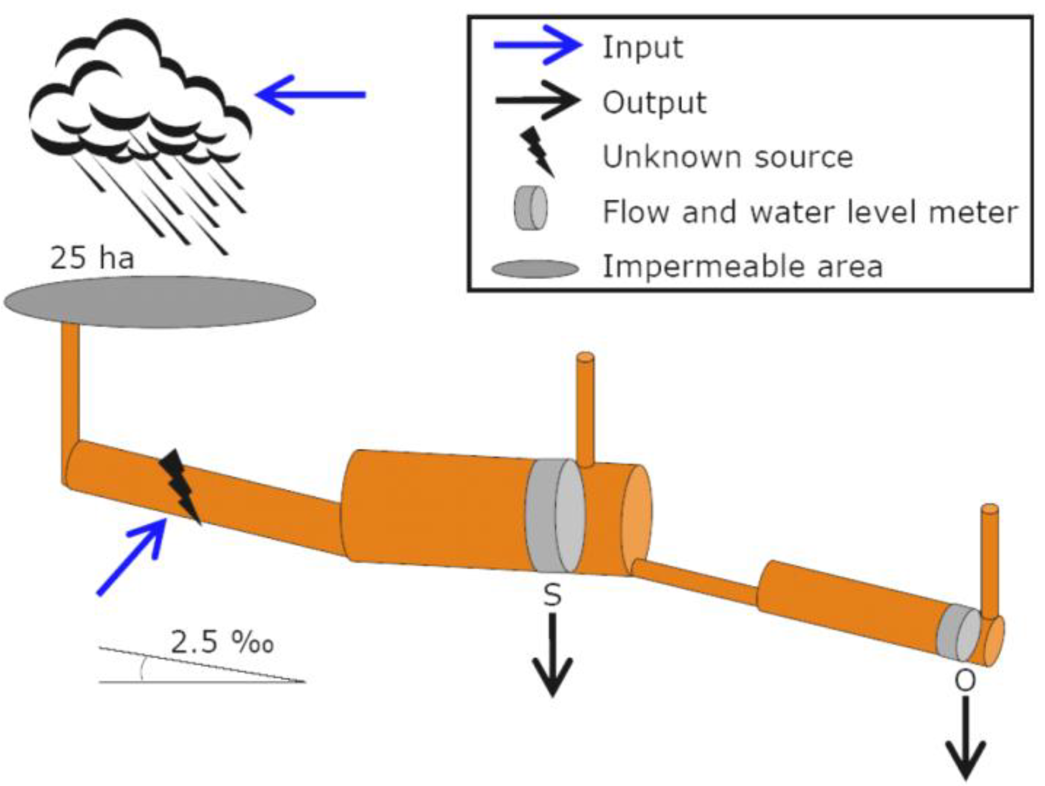
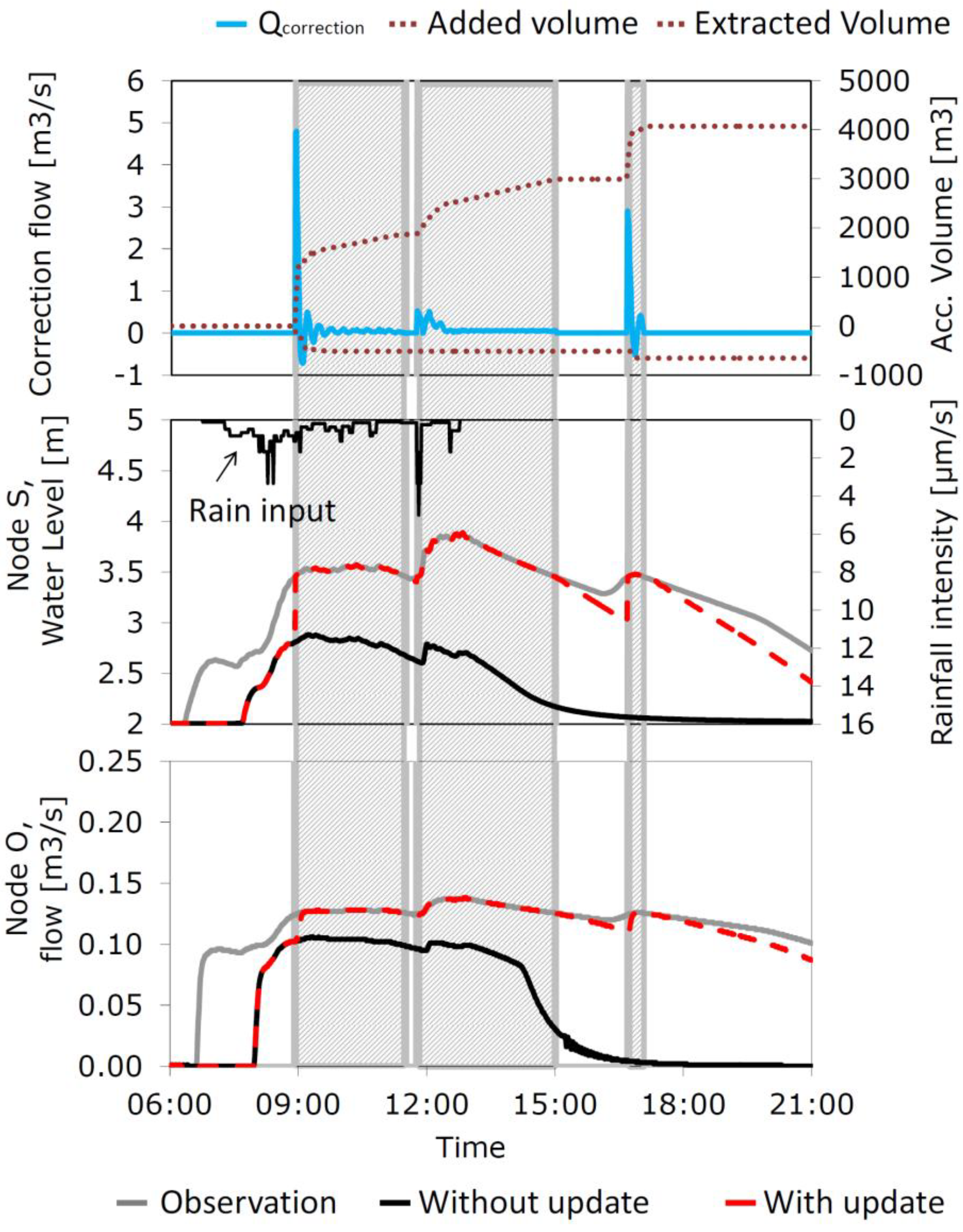
4.1. A Simple Hypothetical Example

A simple hypothetical urban drainage system and a case of defined “unknown input” is set up to illustrate the impact of updating, how level measurements with a limited range can be utilized and that the water balance of the model fits when updating is active. The system consists of six nodes with a storage pipe section in the middle, as illustrated in Figure 3. The storage pipe is horizontal, with invert level at 2.0 m, while the remaining pipes have a 2.5‰ slope. The diameters of the upstream pipe, storage pipe, throttle pipe below the storage pipe and the downstream pipe are 1.5 m, 2 m, 0.35 m and 1 m, respectively, while the total length of the pipe system is 1900 m. Two virtual flow and water level meters are placed within the system – one at the outlet (O) of the system and the other at the outlet of the storage pipe (S). The level meter in the storage pipe (S) records properly when the water level is more than 1.45 m above the bottom of the node (corresponding to a level of 3.45 m), which illustrates a commonly occurring situation when pressure transducers are used for level measurements; these only measure when the water level exceeds the level the gauge has been installed in. The upstream node receives runoff from a catchment with a total impermeable area of 25 hectares, and the outlet of the system has a fixed water level boundary of 0.25 m above the bottom of the outlet.

Figure 3. Illustration of the model setup for the hypothetical example along with input and output locations.

Figure 3. Illustration of the model setup for the hypothetical example along with input and output locations.

To generate artificial observations at S and O a rain event measured by a rain gauge is used along with an inserted flow located in the pipe just before the storage pipe, as shown in Figure 3.

The rainfall-runoff process is modelled using a simple time area method, and the inserted flow represents water unaccounted for in the model due to, for example, infiltration inflow or deviations between actual and measured rainfall. Rain input and additional inflow, which can be seen in Figure 4, generate a set of synthetic water level observations for nodes S and O, where the observations at node S are used for updating the modelled water levels in node S when the observed water level is above 3.45 m.

Figure 4. Rain input and the additional inflow inserted upstream from node S in the hypothetical example, also referred to as the “unknown flow input”.

Figure 4. Rain input and the additional inflow inserted upstream from node S in the hypothetical example, also referred to as the “unknown flow input”.

Figure 5 shows the correction flow and the accumulated correction volumes in node S (top panel), the observed and simulated water level in node S with and without updating in node S (middle panel) and the observed and simulated flow in node O with and without updating in node S (bottom panel). The results are generated using the method described in Section 3.3. The grey-shaded areas indicate periods where updating is active, i.e., where the observed water level is above 3.45 m. The middle panel shows that the simulated water level in node S is equal to the measured level as long as updating is active, and that the water level converges slowly towards the simulated level without update as soon as updating is turned off. A similar pattern can be seen for the downstream flow in node O. As soon as the updating becomes active, the modelled flow quickly resembles the observed flow, and when updating is turned off, the modelled flow converges slowly towards the modelled flow from a normal model run. Hence, the simulation with updating is far better than the simulation entirely without updating.

Figure 5. Three graphs are joined into one in this figure. The top panel shows the correction flow (Q_correction, solid curve) as well as the accumulated volumes inserted and extracted (dotted curves) in node S by updating. In the middle panel, the water level in node S is shown. Both the observed and simulated water levels with and without updating are shown. Rain input can also be seen in the middle panel. The bottom panel shows the observed and the simulated flow with and without updating in node O. In all three graphs the shaded background indicates when updating is activated.

Figure 5. Three graphs are joined into one in this figure. The top panel shows the correction flow (Q_correction, solid curve) as well as the accumulated volumes inserted and extracted (dotted curves) in node S by updating. In the middle panel, the water level in node S is shown. Both the observed and simulated water levels with and without updating are shown. Rain input can also be seen in the middle panel. The bottom panel shows the observed and the simulated flow with and without updating in node O. In all three graphs the shaded background indicates when updating is activated.

The accumulated correction flow in the top panel in Figure 5 shows that a large amount of water is inserted into the model as a result of updating (about 4000 m³ in total), which is expected because the update algorithm has to compensate for the additional inflow representing unaccounted water, as highlighted in Figure 4. The correction flow from updating (Figure 5) shows large variations each time the measured water level rises above 3.45 m and the updating becomes active. This is due to the fact that all compensating water is inserted by the updating algorithm during a single time step, which leads to sudden changes in the water level in one end of the storage pipe and initiates a wave that moves back and forth a couple of times through the pipe. This wave affects the updating algorithm, which attempts to keep the water level at the measured value, and this explains the oscillations in the correction flow seen in Figure 5 as well as the small accumulated volume of water that is extracted during updating. The oscillations only appear as a response to the large and sudden changes in water level caused by the criterion of only updating when the water level is above 3.45 m. After an initial lag-phase, there are no further oscillations in the periods where updating is active. When the updating is continuous, oscillations will thus not appear, and nor will they if the updating happens in an ordinary basin. The oscillations do not seem to have any noticeable downstream impact, and for this simple model they do not give rise to model instability either. For larger models with possible instability issues it might be wise to use an adjustment factor of less than one to ensure a less rapid transition when updating is instantaneously turned on.

The volumes inserted and extracted by the updating illustrated in Figure 5 are 4071 m³ and 652 m³, respectively, resulting in a net volume of 3419 m³ being inserted into the model. The total modelled inflow volume from the rain event without updating is 2430 m³. The ‘unknown’ flow input in this experiment simulation is actually 3450 m³ until the last point in time with active “update”. This magnitude matches the net volume generated by the update method.

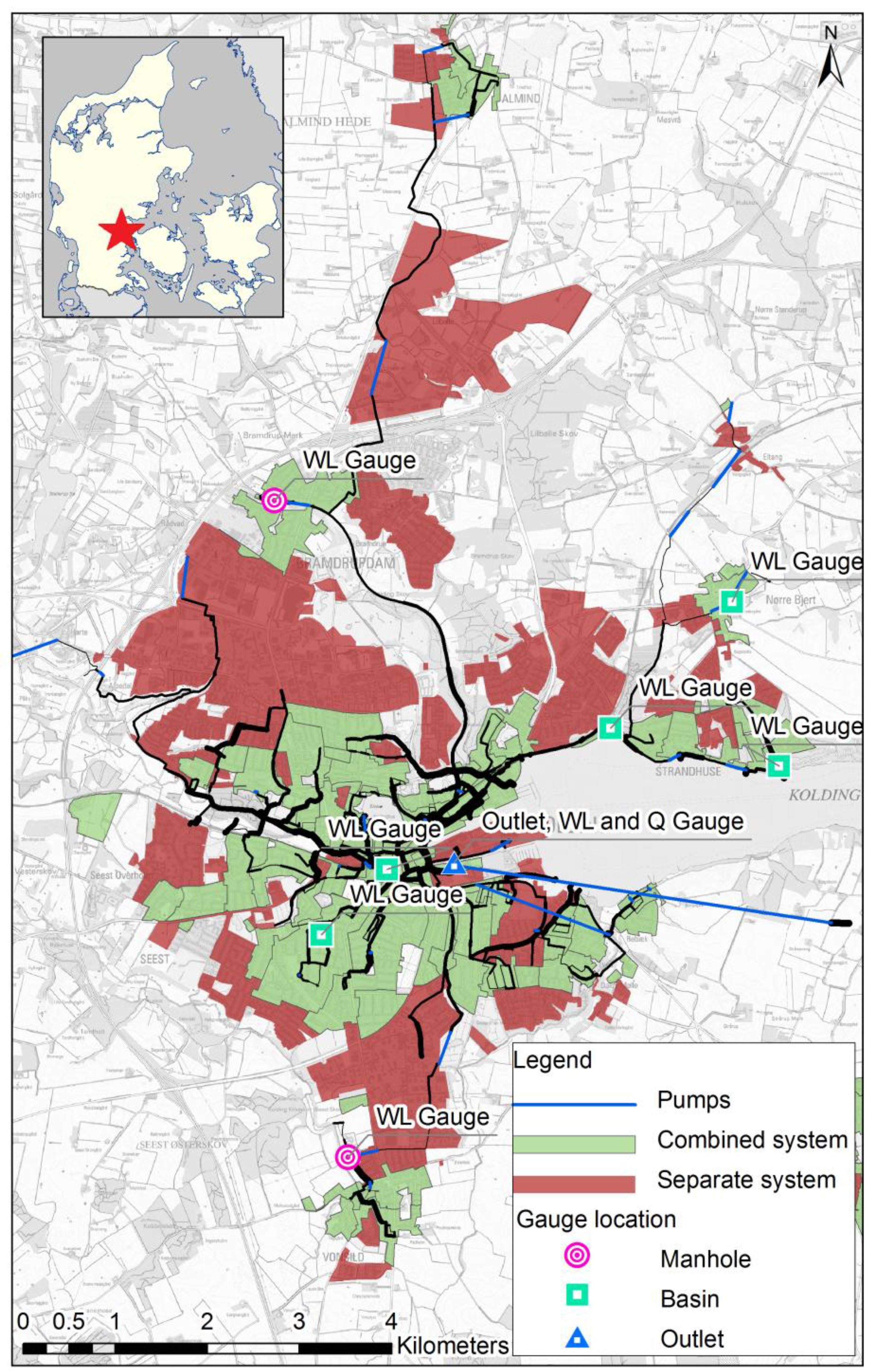
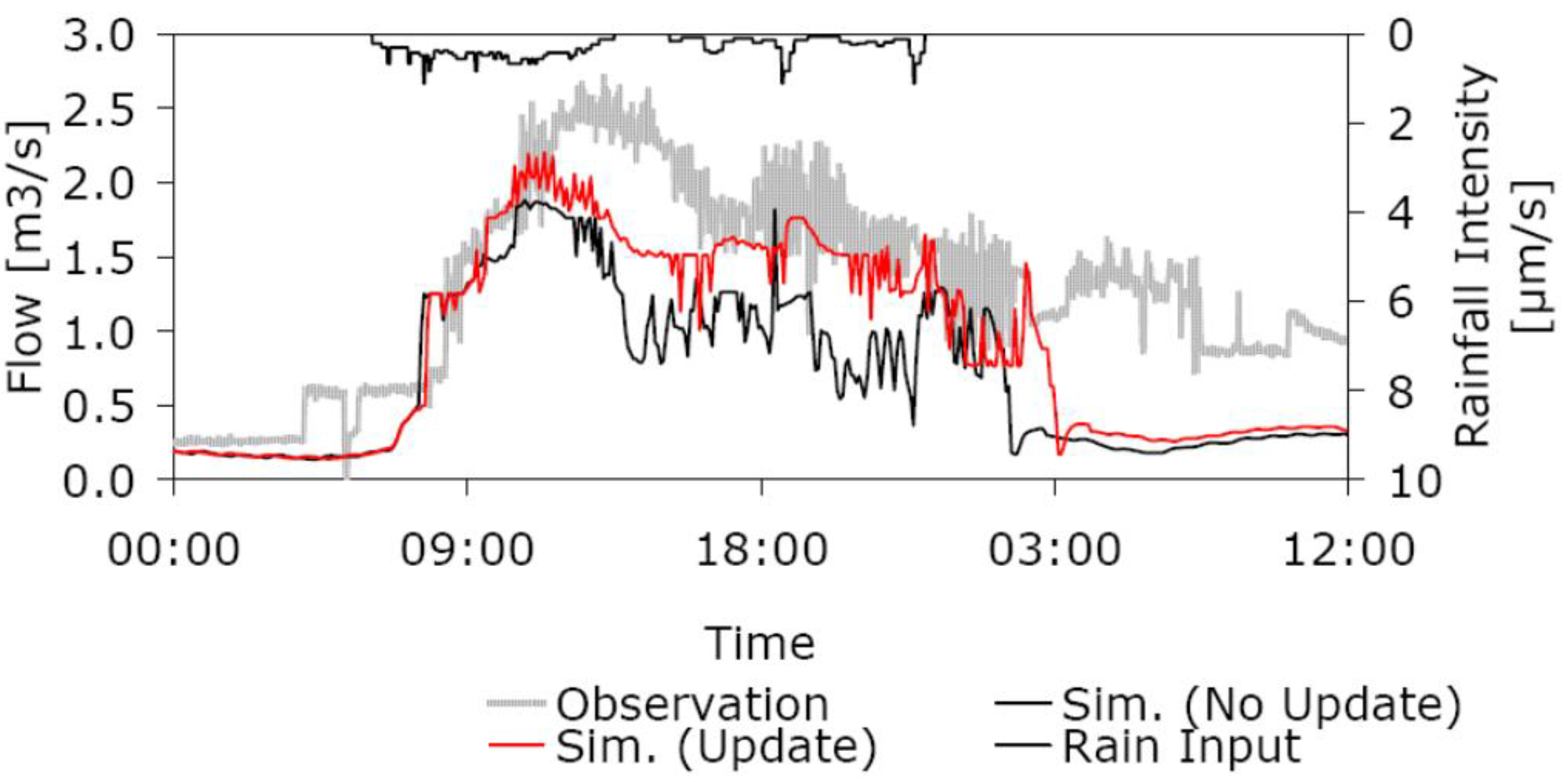
4.2. A Real Full-Scale Example

A model of the urban drainage system in the city of Kolding, Denmark, is used to examine the effects of updating water levels in multiple upstream nodes on the simulation result and the forecast quality at the catchment outlet. All data and model details were provided by the consultancy currently investigating the feasibility of using advanced real time control in the catchment (see Acknowledgements). The model consists of 2303 nodes, 76 pumps, 94 weirs and 1223 sub-catchments with a total impermeable area of 544 ha.

Water levels are updated using measured data in eight different locations, namely six basins and two manholes, as illustrated in Figure 6, and the simulation outputs are compared with the measured flow at the outlet, which is placed near the city center. Most of the water level meters are located close to pumps, which causes the dry weather flow to be dominated by frequent fluctuations. Updating is therefore activated only when the water level is higher than the maximum daily dry weather water level. Data from a single rain gauge located in the city center is used as rain input.

The event used in the simulations is from December 2009 (00:00 25 December to 12:00 26 December), and it represents events that occur very commonly, with a return period below 0.3 years for durations between 1 and 360 min (cf. the national Danish intensity-duration frequency relationship in e.g., [30]). It lasts about a day and a half and has a rain depth of 18 mm. Figure 7 shows the rainfall and the observed and simulated flow at the catchment outlet with and without updating in the upstream basins and manholes. The simulation without updating corresponds well with the measured flow for the first couple of hours of the event, i.e., here updating does not improve the simulations, but then the simulated values without updating drop far below the measured values for the remaining time.

Figure 6. Overview of the distributed urban drainage model for Kolding. The squares, dots and triangles indicate where the observations from the six basins, two manholes and the outlet are located. The green and red areas indicate whether stormwater and wastewater flow in the same pipe (green, the system is combined) or in different pipes (red, the system is separated). Small villages that contribute to the flow are not included on the map.

Figure 6. Overview of the distributed urban drainage model for Kolding. The squares, dots and triangles indicate where the observations from the six basins, two manholes and the outlet are located. The green and red areas indicate whether stormwater and wastewater flow in the same pipe (green, the system is combined) or in different pipes (red, the system is separated). Small villages that contribute to the flow are not included on the map.

The fact that the measured flow continues to be rather high for at least half a day after the rain has stopped indicates that the model error is due to a slow-changing process, such as infiltration or snowmelt, which are processes that are not included in the model. The graph for the updated simulation is much closer to the measured values for a large part of the event, showing that updating in eight upstream locations (6 basins and two manholes, as indicated on Figure 6) to some degree is capable of compensating for the model’s inadequacies. In this case, updating adds about 60% of the water volume that is missing (compare measured and simulated flows ion Figure 7).

Figure 7. Rainfall (from the top, black curve) and observed flow (grey curve) at the outlet in Kolding on 25 and 26 December 2009, along with the simulated flow with (red curve, Update) and without (black curve, No Update) updating in the upstream nodes.

Figure 7. Rainfall (from the top, black curve) and observed flow (grey curve) at the outlet in Kolding on 25 and 26 December 2009, along with the simulated flow with (red curve, Update) and without (black curve, No Update) updating in the upstream nodes.

The period where updating improves the result is between 11:00, 25 December and 03:00, 26 December (Figure 7). The simulation with updating can be used as a reference when evaluating the forecast quality and Figure 8 shows this together with the 30 min (top) and 3 h (bottom) forecasts within this period calculated using the method describes in Section 3.3. The result for the 30 min forecast is very similar to the result for a simulation run with updating. The result for the 3 h forecast is closer to the simulation run without updating until approximately 14:00, 25 December; subsequently, and until around 03:00, 26 December_, the forecasted flow is very similar to the simulated flow when updating. This means that for an almost 12-h period the 3 h forecast (with updating prior to the forecast period) provides results that are closer to the observations than a forecast made without updating. Some discrepancy between the forecasted and observed are however visible, especially for peak flows.

Figure 8. Rainfall (from the top, black curve) and observed flows (grey curves) at the outlet on 25 and 26 December 2009 (part of the hydrograph shown in Figure 7), along with the simulated flow with (red curve, Update) and without (black curves, No Update) updating. The green (a) and blue (b) squares represent the 30 min and 3 h forecast time series, respectively. See Figure 2 for further explanations.

Figure 8. Rainfall (from the top, black curve) and observed flows (grey curves) at the outlet on 25 and 26 December 2009 (part of the hydrograph shown in Figure 7), along with the simulated flow with (red curve, Update) and without (black curves, No Update) updating. The green (a) and blue (b) squares represent the 30 min and 3 h forecast time series, respectively. See Figure 2 for further explanations.

The results show that updating the water level in eight upstream nodes first improves the simulation results for the tail of the hydrograph (Figure 8), while any improvement for the peak flow is rather limited. For updating to have an effect on a simulated flow from a particular part of the system, the water from this area has to run past an updated node. The outlet in Kolding is located near the city center, however, and a lot of the fastest runoff therefore runs directly to the outlet without passing a point with a water level meter. This explains why updating has a very limited effect on peak flow. The total impermeable area upstream of the water level meters is 182 ha, i.e., one-third of the total area, and it is thus the effect of updating only 33% of the flow from the total area that gives this noticeable effect on the outlet flow.

The simulation of both the peak and tail could most likely be improved further by updating in more nodes, but there is a limitation to how much the forecasting of the peak flow can be improved by employing this method. This is due to a lack of basins near the outlet and because the majority of the impermeable area in Kolding is close to the outlet. However, updating in more basins over the entire model area should improve the tail of the hydrograph for the model simulation and the forecast time series.

5. Discussion

The investigated update algorithm is a fairly simple data assimilation tool and has the advantage of being easy to use and being computationally efficient. Since measured water levels are assimilated directly into the model, measurement uncertainties are however transferred to the model. This means that the measurements have to be of good quality, and the use of updating should thus preferably be combined with automated quality control of the measurements, where the raw data from routine monitoring programs are filtered using heuristic or statistical methods e.g., [31] prior to insertion into the Update scheme. Even when the measurements are perfect, direct updating of water levels should be used with care. If the relationship between flow and water level (Q/H-relation) at the update location is not exactly the same in reality as in the model, the consequence of updating the water level in the model will be an erroneous flow into or out of the system. Therefore, updating is best suited for setting the water level in basins where the Q/H-relation in the discharge pipe is well known. In ordinary manholes, the Q/H-relation is much more complex and uncertain, which makes it very likely that updating in these places will cause problems. As an example, a change in water level of 10 cm in a pipe can make a huge difference to the flow through the pipe while the same change in water level in a basin hardly will affect the outflow. Furthermore, the fact that basins store relatively large amounts of water, and empty relatively slowly, makes the effect of updating in these areas significant when producing forecasts. This means that updating generally has a greater potential in catchments with large amounts of storage than in catchments without storage.

The fact that the updating method only updates in the few selected points can give rise to some curious and undesirable effects, due to the possible introduction of large local gradients. If the update scheme is to be used in pipes or storage pipes, care must be taken not to induce oscillations into the system, though this can be handled by setting the adjustment factor to a sufficiently small value.

If the reported correction flows and volumes are large compared to the results from normal simulations, this may be due to a poor calibration of the model or to errors in applied input or measurement data. Updating is thus not a shortcut to bypassing the work on creating a well-calibrated model. If, for instance, the response time of the model upstream of the updating point is far from reality, it will affect the updated model in a way similar to using time-displaced rain data (see e.g., [32]). In this case, the model and the measured values are not synchronized in time and the updating can actually end up worsening the forecasts of the model.

Deterministic updating as investigated here is intended to improve the accuracy of model forecasts in online applications. The success of the method depends on the quality of the model, including its calibration, on the quality of data from the applied level and flow sensors and on the characteristics of the system under consideration. The method introduces changes to the calculations compared with a normal simulation, but all modifications are reported to the results as correction flows and accumulated correction volumes, thus ensuring that water balance validation of the model can still be performed. The only difference is that part of the inflow (or outflow) is not accounted for by physical process description in the model. Nonetheless, this is not a major concern when using a model online, in which case the main priority is to make the model fit to reality.

The proposed updating method is not in any way optimal—but it is feasible and easy to use. A state-of-the-art updating procedure would be capable of weighing up the uncertainty of the measurements against the uncertainty of the modelled values and instantaneously make a system-wide correction to the entire model while producing corresponding uncertainty estimates. Ensemble-based data assimilation methods, such as variants of the Ensemble Kalman Filter, are capable of doing this for non-linear models, but these depend on running large ensembles of models that ideally represent all uncertainty in model and input data. It will presumably take many years before ensemble-based data assimilation methods can be applied successfully to large operational distributed urban drainage models, which are inherently slow and furthermore tend to grow in complexity with the increase in computer power. Until then, the deterministic updating method described in this paper seems like a reasonable compromise. Analysis of further case studies with different characteristics (size, flow time, type and location of measurements) as well as rain storms of varying type (intensity, duration, return period) will contribute to further understanding the method as well as the potentials and disadvantage of using data assimilation in connection with distributed hydrodynamic urban drainage models.

6. Conclusions

The deterministic updating of water levels, as implemented in the MOUSE UPDATE tool investigated here, is a simple tool that works by inserting or extracting enough water at every computational time step into the point of update in the model, to make the modelled values fit the measured value at this specific location. Updating can improve simulation results for the updated node as well as for downstream nodes, as exemplified here by both a hypothetical and a real case study.

The results from a hypothetical test catchment with an unknown infiltration inflow illustrated how the updating works and affects downstream nodes. The results from a real 544 ha catchment showed improved forecasts when updating water levels in six basins and two nodes, even though these represent only flow from 33% of the impermeable catchment area. Our main conclusions are that:

•

Point-wise deterministic updating of water levels in a distributed hydraulic urban drainage model improves model simulations, even in locations where measurements are unavailable, and can thus be used to give a better evaluation of the state of the system than traditional simulations without updating;

•

Updating works best in systems with slow flow dynamics and where updating occurs in multiple upstream basins with slow water level variations, which represent a dominant part of the contributing area;

•

Updating improves forecasts compared to not updating, and there is hence some potential for using updated models in model-based warning and control systems;

•

An example, based on a real full-scale system, shows that a 3 hr forecast with updating provides flow predictions closer to the measured flow than a traditional simulation without updating;

•

Updating of water levels is a pragmatic tool that can help to compensate for the ever-present deviations between model simulations and measured data.

In the future, when computer power has hopefully increased manifold, a simplified data assimilation tool like the one examined in this paper may be replaced by ensemble-based data assimilation methods that additionally produce uncertainty estimates for the entire system. Until then, the investigated Update method may be sufficient for many online applications.

References

1. Fletcher, T.D.; Andrieu, H.; Hamel, P. Understanding, management and modelling of urban hydrology and its consequences for receiving waters: A state of the art. Adv. Water Resour. 2013, 51, 261–279. [Google Scholar] [CrossRef]
2. Wagener, T.; Reed, P.; van Werkhoven, K.; Tang, Y.; Zhang, Z. Advances in the identification and evaluation of complex environmental systems models. J. Hydroinform. 2009, 11, 266–281. [Google Scholar] [CrossRef]
3. Mark, O.; Lacoursiere, J.O.; Vought, L.B.; Amena, Z.; Babel, M.S. Application of hydroinformatics tools for water quality modeling and management: Case study of Vientiane, Lao PDR. J. Hydroinform. 2010, 12, 161–171. [Google Scholar] [CrossRef]
4. Mynett, A.E.; Vojinovic, Z. Hydroinformatics in multi-colours-part red: Urban flood and disaster management. J. Hydroinform. 2009, 11, 166–180. [Google Scholar] [CrossRef]
5. Kalman, R.E. A new approach to linear filtering and prediction theory. Trans. ASME J. Basic Eng. Ser. D. 1960, 82, 35–45. [Google Scholar] [CrossRef]
6. Breinholt, A.; Thordarson, F.O.; Møller, J.K.; Grum, M.; Mikkelsen, P.S.; Madsen, H. Grey-Box modelling of flow in sewer systems with state-dependent diffusion. Environmetrics 2011, 22, 946–961. [Google Scholar] [CrossRef]
7. Breinholt, A.; Møller, J.K.; Madsen, H.; Mikkelsen, P.S. A formal statistical approach to representing uncertainty in rainfall-runoff modelling with focus on residual analysis and probabilistic output evaluation—Distinguishing simulation and prediction. J. Hydrol. 2012, 472–473, 36–52. [Google Scholar] [CrossRef]
8. Evensen, G. Sequential data assimilation with nonlinear quasi-geostrophic model using Monte Carlo methods to forecast error statistics. J. Geophys. Res. 1994, 99, 143–162. [Google Scholar] [CrossRef]
9. Neal, J.C.; Atkinson, P.M.; Hutton, C.W. Flood inundation model updating using an ensemble Kalman filter and spatially distributed measurements. J. Hydrol. 2007, 336, 401–415. [Google Scholar] [CrossRef]
10. Gordon, N.J.; Salmond, D.J.; Smith, A.F.M. Novel approach to nonlinear/non-Gaussian Bayesian state estimation. IEEE Proc. F Radar Signal Proc. 1993, 140, 107–113. [Google Scholar] [CrossRef]
11. Moradkhani, H.; Hsu, K.L.; Gupta, H.; Sorooshian, S. Uncertainty assessment of hydrologic model states and parameters: Sequential data assimilation using the particle filter. Water Resour. Res. 2005, 41. [Google Scholar] [CrossRef]
12. US Environmental Protection Agency: Storm Water Management Model (SWMM). Available online: http://www2.epa.gov/water-research/storm-water-management-model-swmm (accessed on 21 July 2014).
13. MIKE by DHI: MIKE URBAN product page. Available online: http://mikebydhi.com/Products/Cities/MIKEURBAN.aspx (accessed on 21 July 2014).
14. Innovyze: InfoWorks CS product page. Available online: http://www.innovyze.com/products/infoworks_cs (accessed on 21 July 2014).
15. Rambøll; EnviDan; Odense Vandselskab. Intelligent wastewater handling, documentation of phase 2—Implemention, calibration and validation of simulation tools. Rambøll: Copenhagen, Denmark, 2010. (In Danish) [Google Scholar]
16. Festersen, S.H.; Gøtterup, J.G. Monitoring and Modelling of Hydraulics and Water Quality in the Lynette Catchment. Master’s Thesis, Department of Environmental Engineering, Technical University of Denmark, Lyngby, Denmark, 1 August 2013. [Google Scholar]
17. Madsen, H.; Skotner, C. Adaptive state updating in real-time river flow forecasting—A combined filtering and error forecasting procedure. J. Hydrol. 2005, 308, 302–312. [Google Scholar] [CrossRef]
18. Borup, M. Real Time Updating in Distributed Urban Rainfall Runoff Modelling. Ph.D. Thesis, Department of Environmental Engineering, Technical University of Denmark, Lyngby, Denmark, June 2014. [Google Scholar]
19. Hansen, L.S.; Borup, M.; Møller, A.; Breinholt, A.; Mikkelsen, P.S. Performance of MOUSE UPDATE for level and flow forecasting in Urban Drainage Systems. In Proceedings of International MIKE by DHI Conference—Modelling in a World of Change, Copenhagen, Denmark, 6–8 September 2010; p. 11, (CD-ROM).
20. Hansen, L.S.; Borup, M.; Møller, A.; Mikkelsen, P.S. Flow forecasting in urban drainage systems using deterministic updating of water levels in distributed hydraulic models. In Proceedings of the 12th International Conference on Urban Drainage, Porto Alegre, Brazil, 11–16 September 2011; p. 8, (CD-ROM).
21. Thorndahl, S.; Rasmussen, M. Short-term forecasting of urban storm water runoff in real-time using extrapolated radar rainfall data. J. Hydroinform. 2013, 15, 897–912. [Google Scholar] [CrossRef]
22. Borup, M.; Grum, M.; Mikkelsen, P.S. Real time adjustment of slow changing flow components in distributed urban runoff models. In Proceedings of the 12th International Conference on Urban Drainage, Porto Alegre, Brazil, 11–16 September 2011; Full paper PAP005261. p. 8.
23. Abbott, M.B.; Minns, A.W. Computational Hydraulics, 2nd ed.; Ashgate Publishing: Burlington, VT, USA, 1998; p. 557. [Google Scholar]
24. DHI. MOUSE Pipe Flow Reference Manual; DHI: Hørsholm, Denmark, 2011. [Google Scholar]
25. Einfalt, T.; Arnbjerg-Nielsen, K.; Golz, C.; Jensen, N.-E.; Quirmbach, M.; Vaes, G.; Vieux, B. Towards a roadmap for use of radar rainfall data in urban drainage. J. Hydrol. 2004, 299, 186–202. [Google Scholar] [CrossRef]
26. Liguori, S.; Rico-Ramirez, M.A.; Schellart, A.N.A.; Saul, A.J. Using probabilistic radar rainfall nowcasts and NWP forecasts for flow prediction in urban catchments. Atmos. Res. 2012, 103, 80–95. [Google Scholar] [CrossRef]
27. Nielsen, J.E.; Thorndahl, S.; Rasmussen, M.R. A numerical method to generate high temporal resolution precipitation time series by combining weather radar measurements with a nowcast model. Atmos. Res. 2014, 138, 1–12. [Google Scholar] [CrossRef]
28. Rasmussen, M.R.; Thorndahl, S.; Grum, M.; Neve, S.; Borup, M. Weather Radar-Based Control of Wastewater Systems; (In Danish). Miljøministeriet, By- og Landskabsstyrelsen: Copenhagen, Denmark, 2009; ISBN 978-87-92548-28-3. [Google Scholar]
29. Thorndahl, S.L.; Bøvith, T.; Rasmussen, M.R.; Gill, R.S. On combining NWP and radar QPF models for forecasting of urban runoff. IAHS Proc. Rep. 2012, 351, 620–625. [Google Scholar]
30. Madsen, H.; Arnbjerg-Nielsen, K.; Mikkelsen, P.S. Update of regional intensity–duration–frequency curves in Denmark: Tendency towards increased storm intensities. Atmos. Res. 2009, 92, 343–349. [Google Scholar] [CrossRef]
31. Alferes, J.; Tik, S.; Copp, J.; Vanrolleghem, P.A. Advanced monitoring of water systems using in situ measurement stations: Data validation and fault detection. Water Sci. Technol. 2013, 68, 1022–1030. [Google Scholar] [CrossRef]
32. Borup, M.; Grum, M.; Mikkelsen, P.S. Comparing the impact of time displaced and biased precipitation estimates for on-line updated urban runoff models. Water Sci. Technol. 2012, 68, 109–116. [Google Scholar] [CrossRef]
33. Storm- and Wastewater Informatics project homepage. Available online: Available online: www.swi.env.dtu.dk (accessed on 21 July 2014).