Modeling of Soil Water and Salt Dynamics and Its Effects on Root Water Uptake in Heihe Arid Wetland, Gansu, China

Abstract

In the Heihe River basin, China, increased salinity and water shortages present serious threats to the sustainability of arid wetlands. It is critical to understand the interactions between soil water and salts (from saline shallow groundwater and the river) and their effects on plant growth under the influence of shallow groundwater and irrigation. In this study, the Hydrus-1D model was used in an arid wetland of the Middle Heihe River to investigate the effects of the dynamics of soil water, soil salinization, and depth to water table (DWT) as well as groundwater salinity on Chinese tamarisk root water uptake. The modeled soil water and electrical conductivity of soil solution (EC_sw) are in good agreement with the observations, as indicated by RMSE values (0.031 and 0.046 cm³·cm⁻³ for soil water content, 0.037 and 0.035 dS·m⁻¹ for EC_sw, during the model calibration and validation periods, respectively). The calibrated model was used in scenario analyses considering different DWTs, salinity levels and the introduction of preseason irrigation. The results showed that (I) Chinese tamarisk root distribution was greatly affected by soil water and salt distribution in the soil profile, with about 73.8% of the roots being distributed in the 20–60 cm layer; (II) root water uptake accounted for 91.0% of the potential maximal value when water stress was considered, and for 41.6% when both water and salt stress were considered; (III) root water uptake was very sensitive to fluctuations of the water table, and was greatly reduced when the DWT was either dropped or raised 60% of the 2012 reference depth; (IV) arid wetland vegetation exhibited a high level of groundwater dependence even though shallow groundwater resulted in increased soil salinization and (V) preseason irrigation could effectively increase root water uptake by leaching salts from the root zone. We concluded that a suitable water table and groundwater salinity coupled with proper irrigation are key factors to sustainable development of arid wetlands.

1. Introduction

In arid and semi-arid wetlands, salinity and water scarcity are two serious and chronic environmental problems threatening the ecosystem [1]. In the Heihe River basin, China, wetlands are now often experiencing extended periods of high soil salinization levels and associated water availability problems due to the impacts of high evaporative conditions, poor surface drainage, human population pressures, and the associated changes in land use [2,3]. Soil salinity limits plant growth [4] and negatively influences soil quality [5,6], resulting in the change of community structure, density, and growth status. Wetland areas decreased by 42% from 1975 to 2010 within the middle Heihe River basin [7]. Reed marsh areas decreased from 597.8 ha in the late 1990s to the current 492 ha, and that the reed plant height and reed stem were reduced by 25% and 4%, respectively [8]. Owing to the changes in water availability, land desiccation, and salinization, the vegetation has shifted from hydrophytes towards halophytes, psammophytes, xerophytes and super-xerophytes [9]. Meanwhile, soil salinization has caused clogging of soil pores and channels for water flow that has resulted in a considerable reduction in soil permeability, soil porosity, and soil hydraulic conductivity [10]. Consequently, before developing reliable countermeasures, it is important to evaluate the interactions between soil water and salts and their impacts on plant water use, based on factors such as the groundwater quality, the water table, and the plant tolerance to salinity.

In an arid climate where rainfall is very limited, shallow groundwater plays a key role in ecosystem functions. Therefore, it is particularly important to understand the effects of the depth to the water table (DWT) and groundwater quality on root zone water contents, salinity, and plant water use. Jolly et al. [1] concluded that in arid/semiarid environments, where the surface water regime was vulnerable to rainfall variability, the persistence of wetlands can be dependent, either completely or partially, on the contributions from groundwater. Ayars et al. [11] reported that the potential for meeting crop water needs from shallow groundwater ranged up to 50% of the total irrigation. Crops like alfalfa and forage grasses exhibit more continuous water uptake patterns for their long growing seasons and robust root systems [12]. However, most of these previous studies have focused on farmland with few of them giving consideration to wetlands, especially in arid environments [1].

The interactions between the soil water, salt, shallow groundwater, and root water uptake are complex and influenced by numerous factors. Evaluating the interactions of these factors through field research is difficult and time-consuming. In addition, salt variation is often small and is not easily detectable in a single growth season. Simulation models that integrate the soil water movement, solute transport, and plant water uptake provide information that otherwise cannot be obtained from field experiment [13]. Since the 1970s, many numerical solutions were developed to describe water and solute transport [14,15,16]. Most of these models are based on the solutions to the Richards equation for water flow and the convection-dispersion equation (CDE) for solute transport [17]. However, accurate predictions of these models rely on precise measurement of hydraulic characteristics [18]. For some parameters (e.g., α, n and l in the van Genuchten-Mualem function [19,20]), however, it is difficult to measure hydraulic characteristics at the plot scale. Numerous studies have indicated that the laboratory measured hydraulic parameters and/or parameters derived from pedotransfer functions, in combination with inverse optimization algorithms are an effective approach for improving the description of unsaturated hydraulic functions [4,17,21].

In this study, a widely used model Hydrus-1D [22], which simulates one-dimensional transport of water, heat, and multiple solutes in variably saturated media, was adopted to simulate the soil water flow, solute transport and root water uptake in an arid wetland with shallow saline groundwater. Our objectives were: (I) to test the feasibility of the Hydrus-1D model approach in simulating water flow and solute transport with observed data; (II) to characterize the interactions between soil water, salt, and groundwater and their effects on Chinese tamarisk root water uptake and root distribution, and (III) to conduct scenario analyses for the soil water, salt dynamics and root water uptake under different conditions. In addition, the long term salinity trends under different DWTs and groundwater salinities (EC_gw) were investigated.

2. Materials and Methods

2.1. Study Area

The study area is located at Pingchuan town, in the Middle Heihe River basin, Gansu, China (39°20′ N, 100°06′ E). The landform is representative of a riparian wetland covered with Chinese tamarisk, which is the dominant plant community in this area and in the study area served as a shelter forest. Soil electrical conductivities (soil/water ratio of 1/5, EC_1:5) ranged between 1.51 and 26.72 dS·m⁻¹. The DWT ranged from 0.47 m in the rainy fall to 1.44 m in the dry winter. The salinity of the shallow groundwater varied between 2.0 and 4.0 dS·m⁻¹. The climate is a continental arid temperate zone with annual average precipitation of 116.7 mm from 1965 to 2010 with about 60% of the precipitation received during July–September. The annual average potential evaporation is 2366 mm·year⁻¹. The annual average temperature is 7.6 °C, and the lowest and highest temperatures are about −27 °C in January and 39.1 °C in July, respectively [23]. Soil was formed from alluvial deposits with a silty loam texture (Table 1).

Table 1. Soil physical properties and calibrated parameters at the study area.

Soil Layer (cm)	0–15	15–25	25–55	55–65	65–100	100–150
Texture	Silt Loam	Silt Loam	Silt Loam	Silt Loam	Silt Loam	Coarse Sand
Clay (%)	11	10	11	13	16	-
Silt (%)	54	65	66	64	56	-
Sand (%)	35	25	23	23	28	100
Bulk density(g·cm−3)	1.2	1.35	1.42	1.44	1.44	1.42
θr (cm3·cm−3)	0.093	0.08	0.075	0.071	0.079	0.051
θs(cm3·cm−3)	0.543	0.493	0.502	0.462	0.534	0.376
α (cm−1)	0.019	0.028	0.032	0.033	0.035	0.034
n	2.06	1.70	1.50	1.36	1.71	4.43
l	0.5	0.5	0.5	0.5	0.5	0.5
Ks (cm·d−1)	2.5	10.6	24.7	6.7	34.0	1428.0
λ (cm)	16.8	19.5	48.2	29.1	10.8	124.0

Note: The particle size limits were 0.05 to 2 mm for sand, 0.05–0.002 mm for silt and <0.002 mm for clay. θ_r, residual water content; θ_s, saturated water content; α, reciprocal value of air entry pressure; n, the smoothness of pore size distribution; l, pore connectivity parameter; K_s, saturated hydraulic conductivity; and λ, dispersivity.

Table 1. Soil physical properties and calibrated parameters at the study area.

Soil Layer (cm)	0–15	15–25	25–55	55–65	65–100	100–150
Texture	Silt Loam	Silt Loam	Silt Loam	Silt Loam	Silt Loam	Coarse Sand
Clay (%)	11	10	11	13	16	-
Silt (%)	54	65	66	64	56	-
Sand (%)	35	25	23	23	28	100
Bulk density(g·cm−3)	1.2	1.35	1.42	1.44	1.44	1.42
θr (cm3·cm−3)	0.093	0.08	0.075	0.071	0.079	0.051
θs(cm3·cm−3)	0.543	0.493	0.502	0.462	0.534	0.376
α (cm−1)	0.019	0.028	0.032	0.033	0.035	0.034
n	2.06	1.70	1.50	1.36	1.71	4.43
l	0.5	0.5	0.5	0.5	0.5	0.5
Ks (cm·d−1)	2.5	10.6	24.7	6.7	34.0	1428.0
λ (cm)	16.8	19.5	48.2	29.1	10.8	124.0

Note: The particle size limits were 0.05 to 2 mm for sand, 0.05–0.002 mm for silt and <0.002 mm for clay. θ_r, residual water content; θ_s, saturated water content; α, reciprocal value of air entry pressure; n, the smoothness of pore size distribution; l, pore connectivity parameter; K_s, saturated hydraulic conductivity; and λ, dispersivity.

2.2. Measurements

Field data were collected during two growing seasons of Chinese tamarisk (2 May to 27 October 2012 and 2013). Soil water content was measured using a Neutron Moisture Meter (NMM, L520-D, Nanjing, China) every 5 days with a depth interval of 10 cm down to 100 cm. Soil salinity based on the soil diluted extract method (soil/water ratio of 1/5, EC_1:5) was measured every 15 days with a measurement interval of 10 cm down to 90 cm. A shallow monitoring well was installed in the vicinity of the neutron probe to measure DWT every 5 days. The groundwater electrical conductivity (EC_gw) was measured every 15 days. At the beginning of the experiment, undisturbed soil samples (diameter, 5 cm, height 5 cm) from five representative layers were collected for the laboratory measurement of soil bulk density (BD), texture, saturated hydraulic conductivity (K_s) and water content (θ_s). The BD was calculated from the volume-mass relationship for each core sample. Soil texture was determined using the pipette sampling method [24]. K_s values of the undisturbed soil cores were determined using a falling head method [25]. The soil cores were first saturated from the bottom and then submerged in water for 24 h. After weighing, the saturated soil samples were dried at 105 °C to constant mass, and their mass-based saturated soil water content was determined. θ_s values were determined by multiplying saturated mass-based soil water content with BD. In addition, root distribution was measured using a root auger (Eijkelkamp, The Netherlands), and soil cores were sampled in 10 cm depth increments. Root biomass was obtained by washing away soil particles, oven-dried and weighed (Figure 1).

Figure 1. Graphical representation of (a) the root distribution of Chinese tamarisk measured at the start of the 2012 growing season and (b) the average value of soil water (θ) and EC_sw during the 2012 growing season.

Figure 1. Graphical representation of (a) the root distribution of Chinese tamarisk measured at the start of the 2012 growing season and (b) the average value of soil water (θ) and EC_sw during the 2012 growing season.

2.3. Model Simulation

2.3.1. Soil Water Flow and Solute Transport

Simulations of soil water flow and solute transport were performed with Hydrus-1D [22]. This program numerically solves the Richards equation for water flow and uses advection-dispersion equations (CDE) for heat and solute transport in variably saturated porous media. Variably-saturated water flow is described using the Richards’ equation:

$$\frac{\partial \theta }{\partial t}=\frac{\partial }{\partial z}\left[K\left(h\right)\left(\frac{\partial h}{\partial z}+1\right)\right]-S\left(z,t\right)$$

(1)

where θ is soil water content (L³·L⁻³), t is time (T), z is the vertical space coordinate (L), K is the hydraulic conductivity (L·T⁻¹), h is the pressure head (L), S is the sink term accounting for root water uptake (L³·L⁻³·T⁻¹). The unsaturated soil hydraulic properties were described using the van Genuchten-Mualem functional relationships [19,20]:

$$\text{θ}\left(\text{h}\right)=\{\begin{array}{cc}{\text{θ}}_r+\frac{{\text{θ}}_s-{\text{θ}}_r}{{\left(1+{\left|\text{α}h\right|}^n\right)}^m}& h<0\\ {\text{θ}}_s & h\ge 0\end{array}$$

(2)

$$\text{K}\left(\text{h}\right)=K_s{S}_e^l[1-{\left(1-S_e^{1/m}\right]}^2$$

(3)

$$S_e=\frac{\text{θ}-{\text{θ}}_r}{{\text{θ}}_s-{\text{θ}}_r}$$

(4)

where θ_r and θ_s are the residual and saturated water contents (L³·L⁻³), respectively. K_s (L·T⁻¹) is the saturated hydraulic conductivity, α, (L⁻¹) and n represent the empirical shape parameters, m = 1 − 1/n; l is the pore connectivity parameter, which is taken as 0.5 [20]. S_e is the effective saturation.

2.3.2. Solute Transport

The partial differential equations governing equilibrium one-dimensional solute transport under transient flow in variably-saturated medium is defined in Hydrus-1D as:

$$\frac{\partial \text{θ}C}{\partial t}=\frac{\partial }{\partial z}\left(\text{θ}D\frac{\partial C}{\partial z}\right)-\frac{\partial v\text{θ}C}{\partial Z}$$

(5)

where C is the solute concentration of the liquid phase (M·L⁻³). D is the dispersion coefficient (L²·T⁻¹), and v is the average pore water velocity (L·T⁻¹). The dispersion coefficient is defined as (ignoring molecular diffusion):

$$\text{D}=\text{λv}$$

(6)

where λ is dispersivity (L). The dispersivity is viewed as a material constant independent of the flow rate. Since v is obtained from the numerical solution of the water flow model (the water flux q divided by θ), dispersivity is the only solute transport parameter needed for solving the CDE equation.

2.3.3. Root Water Uptake

The potential transpiration rate, T_p (L·T⁻¹), is spread in the root zone according to the normalized root density distribution function, β (z, t) (L⁻¹). The actual root water uptake, S, is obtained from the potential root water uptake (i.e., potential transpiration) S_p, through multiplication with a stress response function α(h, h_φ, z, t) accounting for water and osmotic stresses [26,27] as follows:

$$\text{S}\left(\text{h},h_{\text{φ},}z,t\right)=\text{α}\left(\text{h},h_{\text{φ},}z,t\right)S_p\left(z,t\right)=\text{α}\left(\text{h},h_{\text{φ},}z,t\right)\text{β}\left(z,t\right)T_p\left(t\right)$$

(7)

where stress response function α(h, h_φ, z, t) is a dimensionless function of the soil water (h) and osmotic (h_φ) pressure heads (0 ≤ α ≤1). S_p(z, t) and S(h, h_φ, z, t) are the potential and actual volumes of water removed from a unit volume of soil per unit of time (L³·L⁻³·T⁻¹), respectively. The actual transpiration rate, T_a (L·T⁻¹), is then obtained by integrating Equation (7) over the root domain L_R:

$$T_a=\underset{L_R}{\overset{ }{{\displaystyle \int }}}S\left(\text{h},h_{\text{φ},}z,t\right)dz=T_p\underset{L_R}{\overset{ }{{\displaystyle \int }}}\text{α}\left(\text{h},h_{\text{φ},}z,t\right)\text{β}\left(z,t\right)dz$$

(8)

We further assumed that the effects of water and salinity were multiplicative [28]: α(h, h_φ) = α(h) α(h_φ), so that different stress response functions could be used. Root water uptake due to water stress was described using the model introduced by Feddes et al. [26]:

$${\text{α}}_h=\{\begin{array}{cc}0, & h>h_1, h\le h_4\\ \frac{h-h_1}{h_2-h_1},& h_2<h\le h_4\\ 1, & h_3<h\le h_2\\ \frac{h-h_4}{h_3-h_4},& h_4<h\le h_3\end{array}$$

(9)

where root water uptake is assumed to be zero close to saturation (i.e., wetter than the “anaerobiosis point”, h₁). For h < h₄ (the wilting point pressure head), root water uptake is also completely stressed. Root water uptake is considered to be at the potential rate when pressure heads range from h₂ to h₃, and when pressure head values are between h₁ and h₂ (or h₃ and h₄), root water uptake increases (or decreases) linearly with h.

Hydrus-1D assumes h₃ is a function of T_p and allows users to specify two different T_p (T_p1 and T_p2) and h₃ (h_3-1 and h_3-2), respectively. The calculation equations are:

$$h_3=\{\begin{array}{cc}{h}_{3-1}+\frac{\left(h_{3-2}-h_{3-1}\right)}{\left(T_{p1}-T_{P2}\right)\left(T_{p1}-T_p\right)}& T_{p2}<T_p<T_{p1}\\ h_{3-2} & T_p<T_{p2}\\ h_{3-1} & T_p>T_{p1}\end{array}$$

(10)

Root water uptake due to osmotic stress was described with an S-shaped function developed by van Genuchten, 1987 [28]:

$${\text{α}}_{\text{φ}}=\frac{1}{1+{\left(\frac{h_{\text{φ}}}{h_{\text{φ}50}}\right)}^p}$$

(11)

where p represents experimental constants. The exponent p was found to be approximately 3 when only salinity stress data was applied [28]. The parameter h_φ50 represents the pressure head at which the water extraction rate is reduced by 50% during conditions of negligible water stress.

In Hydrus-1D, EC is expressed as electrical conductivity of soil solution (EC_sw). Alternatively, we measured EC_1:5 and converted it into the saturated paste extracts (EC_e) using the following relationship where EC_e = (2.46 + 3.03 θ_sp⁻¹) EC_1:5, where θ_sp is the water content of the saturated paste (θ_sp Kg·Kg⁻¹) [29]. Then EC_e values are converted into EC_sw by the following equation [30]:

$$E{C}_{sw}=E{C}_e\frac{BD\cdot SP}{100\cdot \text{θ}}=E{C}_e\frac{{\text{θ}}_s}{\text{θ}}$$

(12)

where SP is the saturation percentage (the water content of the saturated soil-paste, expressed on a dry-weight basis), BD is the bulk density (g·cm⁻³) and θ_s is the saturated soil water content (L³·L⁻³).

Furthermore, Hydrus-1D uses the following relationship to convert EC_sw to osmotic pressure head (cm):

$$h_{\text{φ}}=-3.8106E{C}_{sw}+0.5072$$

(13)

The equation is very similar to the relationship reported by the US Salinity Laboratory Staff (1954) [31] for estimating the osmotic pressure of soil solutions from EC measurements (h_φ = −3.7188 EC_sw).

2.4. Initial and Boundary Condition

Initial conditions were set in the model with measured soil water contents and electrical conductivities on 2 May 2012. At the soil surface, an atmospheric boundary condition was specified using the daily data of precipitation and reference crop evapotranspiration (ET₀) obtained from the Linze Station (2 km away from the site). Daily values of the ET_p were calculated using the reference evapotranspiration (ET₀) via Penman-Monteith method [32] multiplying by a crop coefficient of the investigated Chinese tamarisk. The crop coefficient was estimated from fraction of ground cover and plant height [33], that is, crop coefficient for the middle season is 1.05, increased from 0.55 to 1.05 linearly in the first 10 days of plant development and decreased from 1.05 to 0.55 linearly in the last seven days of plant defoliation. Then, ET_p was divided into potential evaporation (E_p) and potential transpiration (T_p) according to Beer’s Law:

$$E_p\left(t\right)=E{T}_p\left(t\right)\cdot ex{p}^{-k\cdot LAI\left(t\right)}$$

(14)

$$T_p\left(t\right)=E{T}_p\left(t\right)-E_p\left(t\right)$$

(15)

where k is an extinction coefficient set to be 0.463 and LAI is the leaf area index. The model was used to directly calculate actual E and T given the soil moisture conditions and the root water uptake functions. LAI values were measured during different stages of the growing season using a LI-COR area meter (Model LI-3100C, LI-COR Environmental and Biotechnology Research Systems, Lincoln, Nebraska), and were linearly interpolated between the measurement dates. At the bottom, variable pressure head and concentration boundary conditions were specified for water flow and solute transport using the measured water table depths and groundwater EC, respectively. For solute transport, we assumed that the rain water was free of solutes and implemented a no flux boundary condition at the soil surface. The boundary conditions used in the calibration and validation processes are shown in Figure 2.

Figure 2. Dynamics of potential evapotranspiration, precipitation, depth to water table (DWT) and groundwater electric conductivity (EC_gw).

Figure 2. Dynamics of potential evapotranspiration, precipitation, depth to water table (DWT) and groundwater electric conductivity (EC_gw).

2.5. Model Calibration and Validation

In this study, the Hydrus-1D model was calibrated using site-specific boundary conditions and measured water contents, θ, and electrical conductivities, EC_sw values during 2012. Saturated water content (θ_s) and hydraulic conductivity (K_s) were determined from the soil cores taken as stated above. The other van Genuchten-Mualem parameters were estimated via Rosetta pedotransfer functions [34] using the particle size distribution and bulk density dataset. For initial values of solute transport parameters in the root zone (0–100 cm), the dispersivity (λ) was set to an average value (8.9) based on 67 soils with silt loam textures according to Vanderborght and Vereecken [35]. Based on aquifer materials, thickness, and hydraulic conductivity, the dispersivity of the aquifer was fixed as 124 cm according to Gelhar et al. [36].

The parameters of the Feddes model were synthesized based on Moayyad [37] with Grinevskii [38]: h₁ = −0.1 cm, h₂ = −2 cm, h_3-1 = −80 cm, h_3-2 = −250 cm, h₄ = −15,000 cm. Without consideration of the water stress (i.e., reset the Feddes model parameters to make water stress vanish), parameters of the S-shaped function developed by van Genuchten were fitted as: h_φ50 = 326.4 cm, p = 3. Root distribution was specified according to measured root dry weight distribution along the soil profile (Figure 1).

In Hydrus, inverse parameter estimation employed a relatively simple, gradient-based, local optimization approach based on the Marquardt-Levenberg method [39]. In this case, inverse solutions were used to optimize soil hydraulic and solute transport parameters simultaneously using the observed data, initial conditions, initial estimates, and boundary conditions. That is, α, n and λ in the five upper soil layers were fitted first since Hydrus could optimize 15 parameters at a time. θ_r was the last parameter estimated. Then, the model was validated with the observed data of the 2013 growing season without changing the calibrated parameters.

The agreement between the predicted and observed data was evaluated by root mean square error (RMSE) and coefficient of determination (R²):

$$RMSE=\sqrt{\frac{{{\displaystyle \sum }}_{i=1}^N{\left(O_i-P_i\right)}^2}{N-1}}$$

(16)

$$R^2=1-\frac{{{\displaystyle \sum }}_{i=1}^N{\left(P_i-O_i\right)}^2}{{{\displaystyle \sum }}_{i-1}^N{\left(O_i-\overline{O}\right)}^2}$$

(17)

where O_i and P_i are the ith values of observed and predicted values, respectively, and $\overline{O}$ is the average of observed values. N is the number of observations.

2.6. Simulation Scenarios

In order to understand the impacts of groundwater change on plant water use, we simulated root water uptake under different DWTs and EC_gw conditions. Taking the data of 2012 as the reference, eight DWT (i.e., DWT would either raise or drop 15%, 30%, 45% and 60% based on the 2012 reference depth, respectively) and eight EC_gw (i.e., EC_gw would either increase or decrease 15%, 30%, 45% and 60% based on the 2012 reference value, respectively) were assumed in this process (Table 2).

In addition, to evaluate long-term salinity trends, a long-term time series analysis was conducted considering the fluctuations of DWT and EC_gw in relation to 2012 base values. Firstly, using the LARS-WG weather generator [40] and historical meteorological data from 1954 to 2012, we generated 30 years of weather data which had the same statistical characteristics as the historical data. Then, soil salinization risks were assessed using the generated long-term time series data for three water levels (DWT is 60, 100 (average water level of 2012) and 140 cm) and three groundwater electrical conductivities (EC_gw is 1.75, 3.75 (average EC_gw of 2012) and 5.75 dS·m⁻¹). The initial value of EC_sw was taken as 3.75 dS·m⁻¹ for different water tables and 107.25 dS·m⁻¹ (average root zone EC_sw of 2012) for different EC_gw, respectively.

Salt normally accumulated before the plant germination in our studied area (i.e., the dry and cold winter time). In order to elucidate the impacts of artificial watering on soil water, salt dynamics, and to determine how to alleviate salt stress on the arid wetlands, we evaluated the influence of a preseason irrigation event applied at the initial stages of plant growth starting on 2 May 2012. To account for irrigation amounts ranging from 1 to 80 cm, eighty Hydrus simulation scenarios were run. All simulation scenarios are listed in Table 2.

Table 2. Simulation scenarios performed in this study.

Main Scenarios	Scenarios in Detail
Root water uptake predictions	Depth to water table raise 15% of the 2012 reference depth, DWT+15%
	Depth to water table raise 30% of the 2012 reference depth, DWT+30%
	Depth to water table raise 45% of the 2012 reference depth, DWT+45%
	Depth to water table raise 60% of the 2012 reference depth, DWT+60%
	Depth to water table drop 15% of the 2012 reference depth, DWT-15%
	Depth to water table drop 30% of the 2012 reference depth, DWT-30%
	Depth to water table drop 45% of the 2012 reference depth, DWT-45%
	Depth to water table drop 60% of the 2012 reference depth, DWT-60%
	Groundwater electrical conductivity increase 15% of the 2012 reference value, ECgw+ 15%
	Groundwater electrical conductivity increase 30% of the 2012 reference value, ECgw+ 30%
	Groundwater electrical conductivity increase 45% of the 2012 reference value, ECgw+ 45%
	Groundwater electrical conductivity increase 60% of the 2012 reference value, ECgw+ 60%
	Groundwater electrical conductivity decrease 15% of the 2012 reference value, ECgw− 15%
	Groundwater electrical conductivity decrease 30% of the 2012 reference value, ECgw− 30%
	Groundwater electrical conductivity decrease 45% of the 2012 reference value, ECgw− 45%
	Groundwater electrical conductivity decrease 60% of the 2012 reference value, ECgw− 60%
Long term (30 years) salinity trends	Depth to water table is 60 cm, DWT = 60 cm
	Depth to water table is 100 cm, DWT = 100 cm
	Depth to water table is 140 cm, DWT = 140 cm
	Groundwater electrical conductivity is 1.75 dS/m, ECgw = 1.75 dS/m
	Groundwater electrical conductivity is 3.75 dS/m, ECgw = 3.75 dS/m
	Groundwater electrical conductivity is 5.75 dS/m, ECgw = 5.75 dS/m
Preseason irrigation strategy	A human irrigation (irrigation amount range from 1 to 80 cm) applied at the initial stages of plant growth (2 May 2012).

Table 2. Simulation scenarios performed in this study.

Main Scenarios	Scenarios in Detail
Root water uptake predictions	Depth to water table raise 15% of the 2012 reference depth, DWT+15%
	Depth to water table raise 30% of the 2012 reference depth, DWT+30%
	Depth to water table raise 45% of the 2012 reference depth, DWT+45%
	Depth to water table raise 60% of the 2012 reference depth, DWT+60%
	Depth to water table drop 15% of the 2012 reference depth, DWT-15%
	Depth to water table drop 30% of the 2012 reference depth, DWT-30%
	Depth to water table drop 45% of the 2012 reference depth, DWT-45%
	Depth to water table drop 60% of the 2012 reference depth, DWT-60%
	Groundwater electrical conductivity increase 15% of the 2012 reference value, ECgw+ 15%
	Groundwater electrical conductivity increase 30% of the 2012 reference value, ECgw+ 30%
	Groundwater electrical conductivity increase 45% of the 2012 reference value, ECgw+ 45%
	Groundwater electrical conductivity increase 60% of the 2012 reference value, ECgw+ 60%
	Groundwater electrical conductivity decrease 15% of the 2012 reference value, ECgw− 15%
	Groundwater electrical conductivity decrease 30% of the 2012 reference value, ECgw− 30%
	Groundwater electrical conductivity decrease 45% of the 2012 reference value, ECgw− 45%
	Groundwater electrical conductivity decrease 60% of the 2012 reference value, ECgw− 60%
Long term (30 years) salinity trends	Depth to water table is 60 cm, DWT = 60 cm
	Depth to water table is 100 cm, DWT = 100 cm
	Depth to water table is 140 cm, DWT = 140 cm
	Groundwater electrical conductivity is 1.75 dS/m, ECgw = 1.75 dS/m
	Groundwater electrical conductivity is 3.75 dS/m, ECgw = 3.75 dS/m
	Groundwater electrical conductivity is 5.75 dS/m, ECgw = 5.75 dS/m
Preseason irrigation strategy	A human irrigation (irrigation amount range from 1 to 80 cm) applied at the initial stages of plant growth (2 May 2012).

3. Results and Discussion

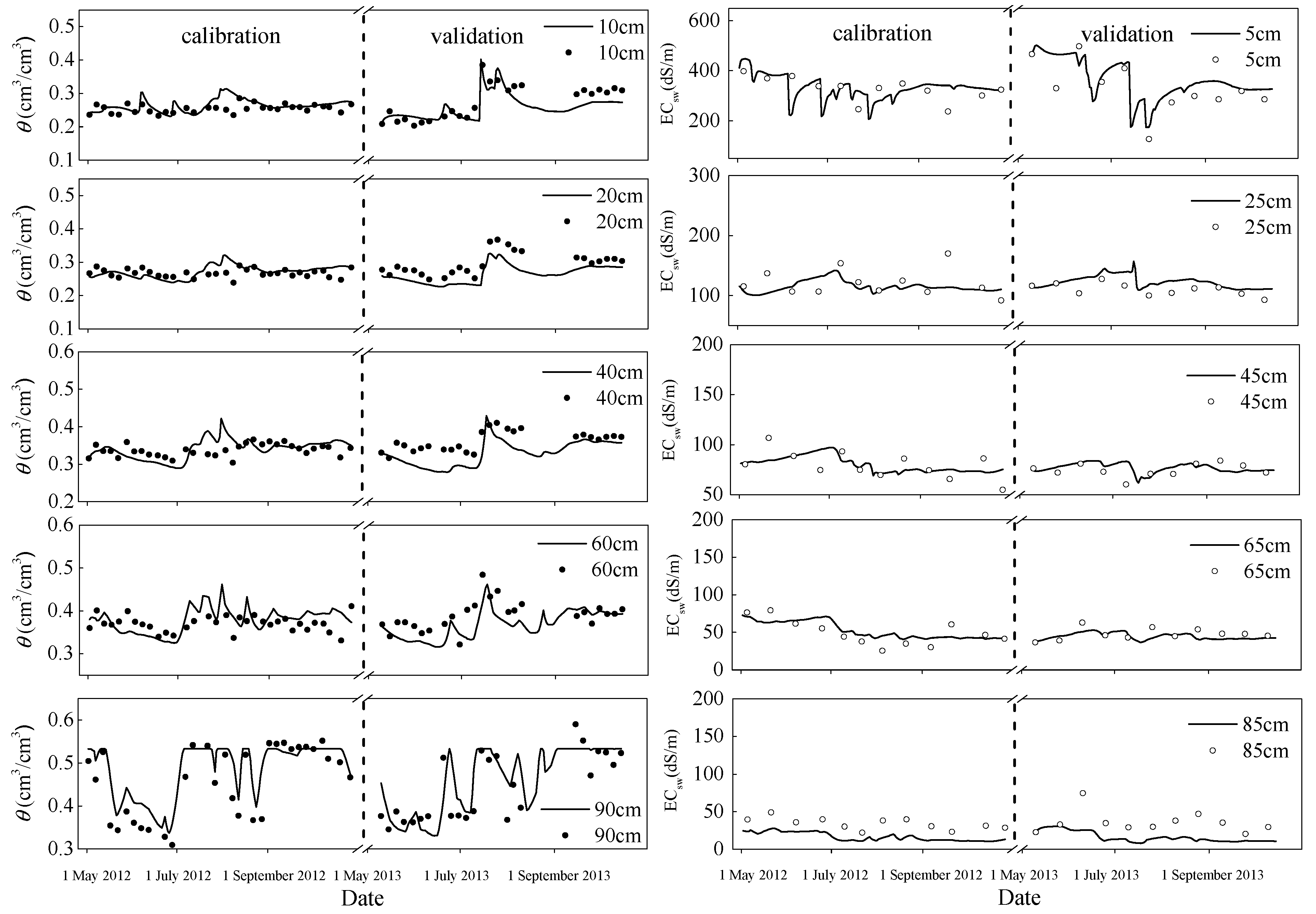
3.1. Model Calibration and Validation

There was good agreement between observed and simulated soil water contents and salt contents as indicated by the smaller RMSE and higher R² values. Calibration periods resulted in RMSE = 0.031 cm³·cm⁻³ and R² = 0.88 for soil water and RMSE = 0.037 dS·m⁻¹ and R² = 0.92 for EC_sw. Validation period resulted in RMSE = 0.046 cm³·cm⁻³ and R² = 0.82 for soil water and RMSE = 0.035 dS·m⁻¹ and R² = 0.95 for EC_sw. These results demonstrated that despite the considerable demands on input data, Hydrus-1D was an effective tool for evaluating water and solute transport [41,42,43] and would be acceptable in performing scenario simulations. The calibrated parameters are shown in Table 1. There was generally very good agreement between the simulated and measured soil water contents, though there are some discrepancies. It is not possible to specifically identify the causes of the discrepancies, but they might be partially attributable to preferential flow caused by macropores and cracks [44,45], spatial heterogeneity and observation errors [46], and the locally occurring chemical processes, such as adsorption-desorption, and proportional root uptake [22], and precipitation/dissolution reactions in soils [47].

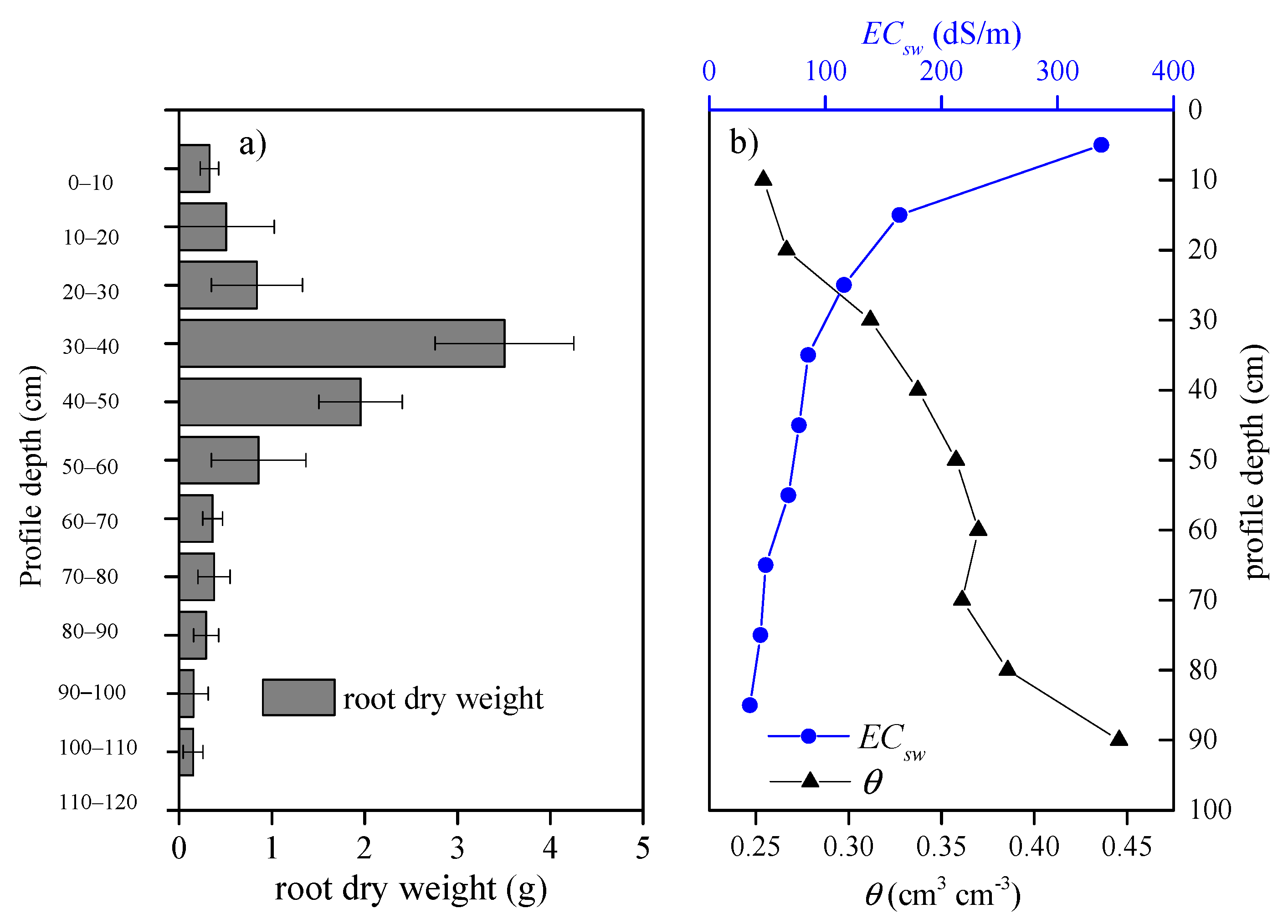
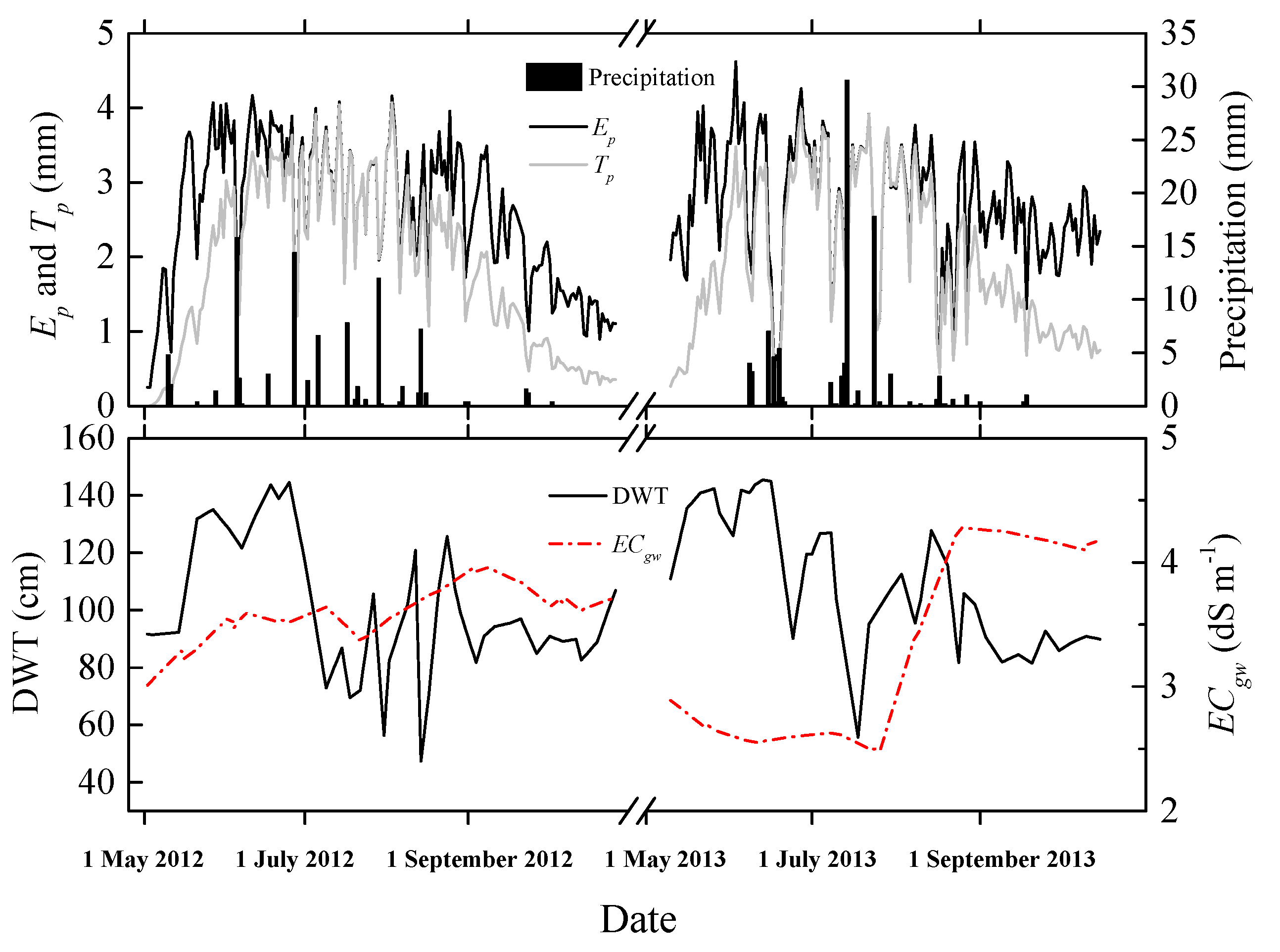
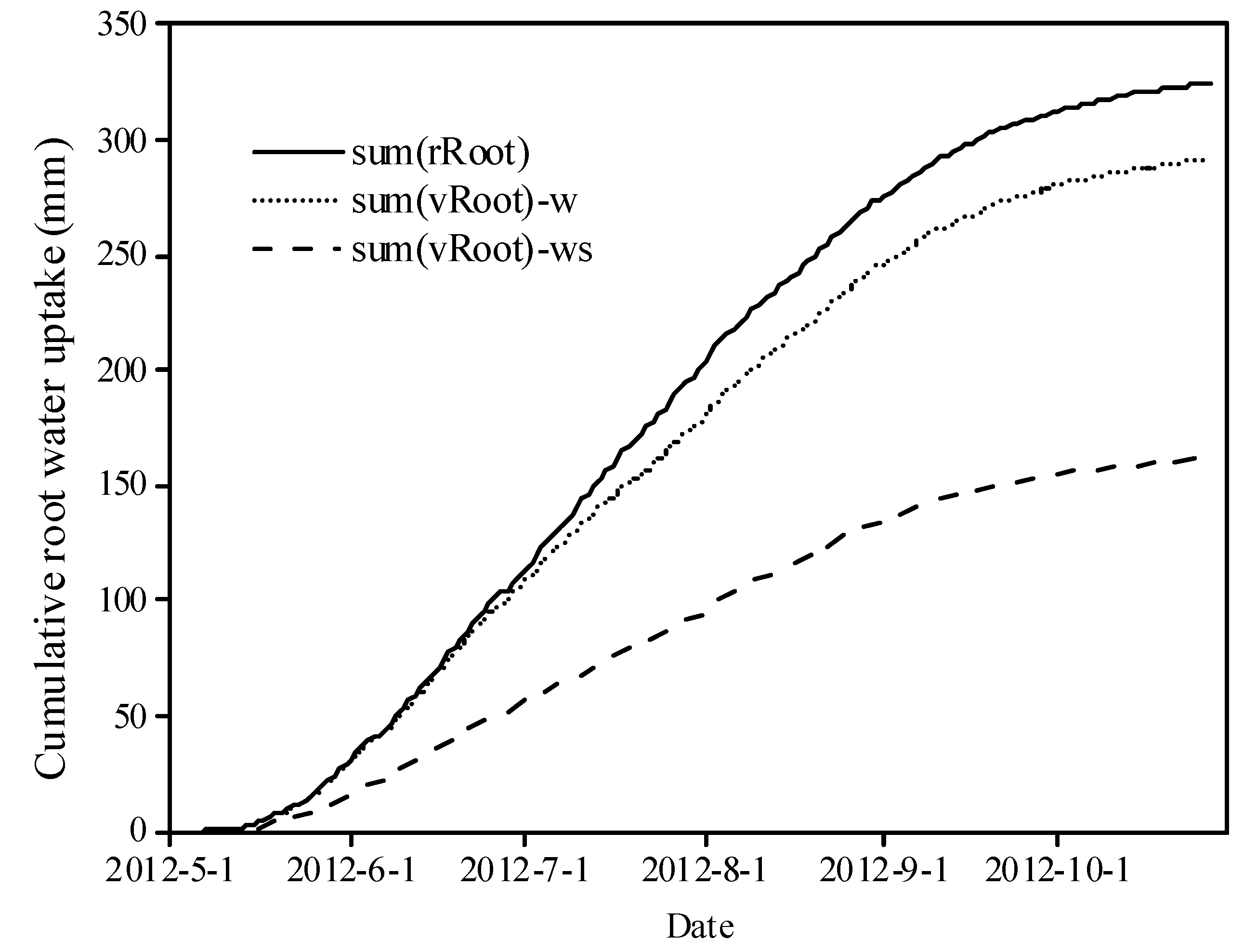
3.2. Soil Water and Salt Dynamics and Their Effects on Root Water Uptake of Tamarisk

The roots of Chinese tamarisk are primarily distributed in the 20–60 cm soil layer, accounting for 73.76% of total dry weight (Figure 1a) with the maximum values (35.55%) at the 30–40 cm soil depth. This distribution may be partially attributed to a large salt accumulation near the soil surface that is unfavorable to root growth (Figure 1b). The accumulation of salts has primarily been caused by high atmospheric demands that caused water movement towards the soil surface from the shallow saline groundwater. Since the groundwater has high salinity levels, salts are also transported with the water and accumulated in the root zone. In addition, scarce rainfall and poor surface drainage have also been shown to contribute to this process in arid regions [48]. Our results are consistent with the reports of Li et al. [49], who found that root growth of tamarisk seemed to be repressed when the salinity (EC_1:5) was greater than 6 dS·m⁻¹. Similarly, although the deeper soil layer contains little salt, shallow water table results in relatively high water contents and small values of aeration porosity. These conditions may limit root growth, respiration, and water uptake. Therefore, the optimum depth observed for plant growth was between 20 to 60 cm, because of the salt stress near the soil surface, and the saturation and anaerobic conditions below the 60 cm soil depth (Figure 3). Therefore, the long-term effects of water and salt stress caused Chinese tamarisk to develop its root system in the most suitable strata.

Figure 3. Measured and simulated soil water and EC_sw in both calibration and validation period during the growing season of Chinese tamarisk.

Figure 3. Measured and simulated soil water and EC_sw in both calibration and validation period during the growing season of Chinese tamarisk.

Dynamics of the profiled water contents were primarily attributable to the natural precipitation, evapotranspiration, and location of the water table. In general, soil water contents increased from the surface layer to the bottom layer because of a shallow water table. The soil moisture at the 20–60 cm strata remained relatively constant during the growing season and served as a soil moisture buffer layer (Figure 1 and Figure 3). Because of the shallow groundwater tables, the soil moisture fluctuated dramatically for the 80–100 cm layer and ranged from 0.33 to 0.53 cm³·cm⁻³ (Figure 3). Similarly, due to the relatively limited precipitation and large quantity of evaporation during 2012, the EC fluctuated intensively with EC_sw values ranging from 207.1 to 448.4 dS·m⁻¹ in the surface layer. Meanwhile, EC decreased from the surface layer to the bottom layer because of the intensive evaporation, poor surface drainage, and negligible precipitation (Figure 1 and Figure 3).

Because of the sparse vegetative cover that was effected by water and salinity stresses, cumulative evaporation reached 149 mm during the growing season. Accordingly, the migration of salt with intensive evapotranspiration was thought to be the main cause for soil salinization in this area. Infiltration was only 91 mm during the 2012 growing season that was less than both evaporation and transpiration (Figure 4). Furthermore, rainfall infiltration could dissolve large quantities of soluble salts from the upper layer. Though precipitation in this region is unable to provide sufficient water for plant growth, cumulative upward soil water flux attributable to groundwater charge reached 216 mm during the growing season of 2012. Further, compared with the infiltration water from the upper boundary, the recharged water from the groundwater has a low salt concentration and can be easily utilized by plant roots. Therefore, the groundwater plays a critical role in the maintenance of Chinese tamarisk growth and water supplements. These observations are in agreement with Morris and Collopy [50], who reported that more than half the tree water uptake (Eucalyptus Camaldulensis and Casuarina cunninghamiana) was drawn from the groundwater. Satchithanantham et al. [51] found that during the dry mid-season, when the ET was at its peak, the groundwater supplied up to 92% of the water for consumptive use by potatoes. Ayars et al. [11] observed that almost 100% of the consumptive use by alfalfa was supplied by contributions from the shallow groundwater.

Figure 4. Cumulative water flux during the growing season of 2012.

Figure 4. Cumulative water flux during the growing season of 2012.

Root water uptake reached 91.0% of its potential maximal value when water stress was considered and only 41.6% of that amount when both water and salt stress conditions were taken into consideration (Figure 5). This phenomenon has been attributed to the vast quantities of soluble salts that results in decreased solute potentials and increased ion toxicity [52]. These types of observations have resulted in assessments of salt stress being the dominating factor affecting root water uptake in arid riparian wetlands [1]. Therefore, there is a pressing need to develop appropriate management measures to reduce the impacts of water and salt stresses on Chinese tamarisk.

Figure 5. Cumulative root water uptake under different stress conditions. Note: sum(rRoot), potential cumulative root water uptake; sum(vRoot)-w, cumulative root water uptake under water stress only; sum(vRoot)-ws, cumulative root water uptake under coupled water and salt stress.

Figure 5. Cumulative root water uptake under different stress conditions. Note: sum(rRoot), potential cumulative root water uptake; sum(vRoot)-w, cumulative root water uptake under water stress only; sum(vRoot)-ws, cumulative root water uptake under coupled water and salt stress.

3.3. Scenario Simulations

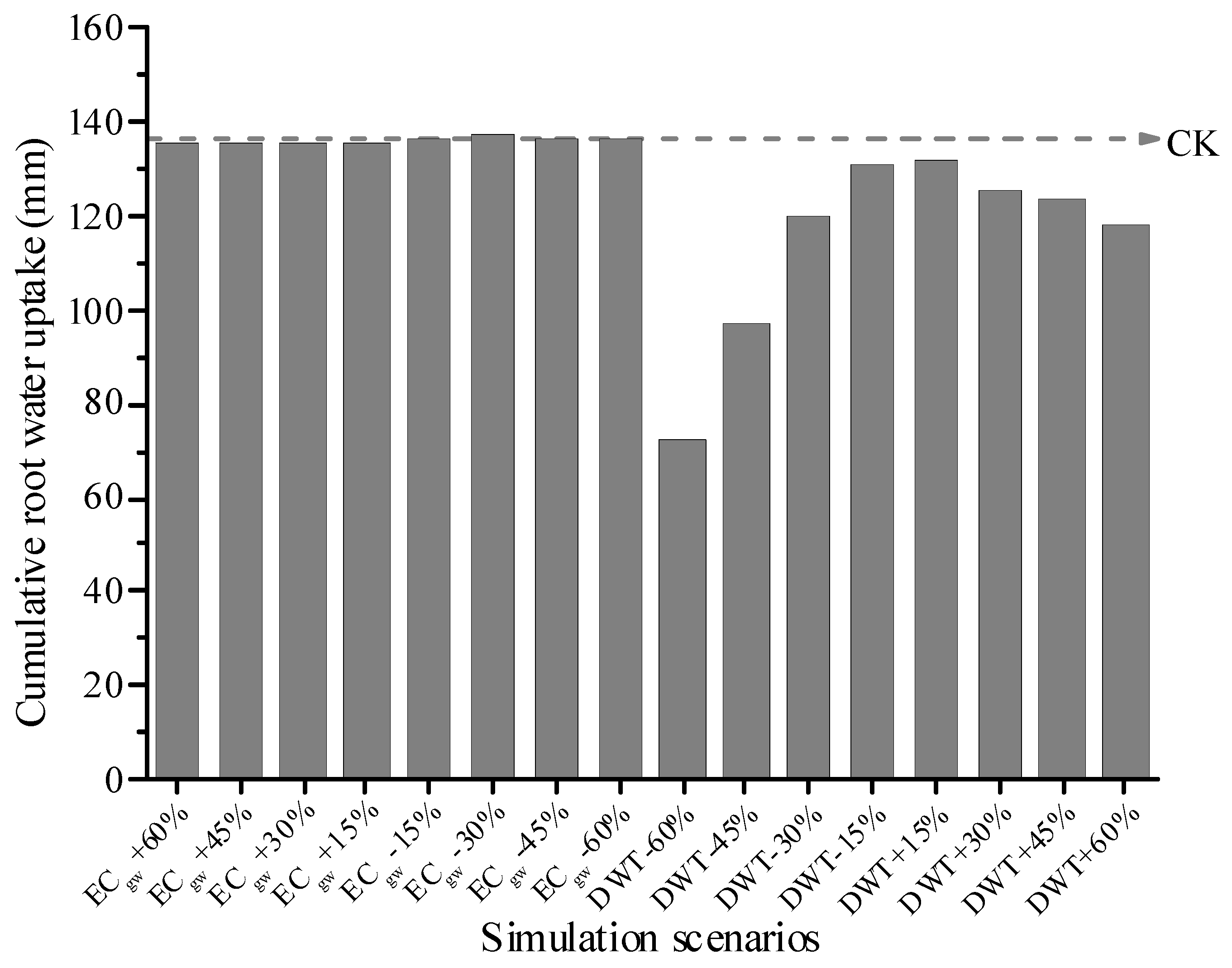
3.3.1. Root Water Uptake Predictions

As indicated by Figure 6, cumulative root water uptake is more sensitive to fluctuations of water table than EC_gw. Root water uptake reached the maximum values of 136.6 mm when DWT was at the 2012 reference depth (CK), then decreased gradually as the water table rose. Cumulative root water uptake only reached 72.5 mm when DWT dropped 60% (DWT − 60%). This reduction in root water uptake was mainly because excessive shallow water table caused water stress in the root zone. Similarly, the cumulative root water uptake declined dramatically when the DWT increased from the 2012 reference depth to DWT + 60%. The cumulative root water uptake only reached 118.6 mm when DWT increased 60%. These simulation results suggest that either too shallow or too deep a water table will have dramatic impacts on the root water uptake. Contrary to the effects of groundwater table, root water uptake exhibited almost no change within the assumed range of EC_gw values. This relative lack of response may be partially attributed to a high degree of salt tolerance for this plant. For example, in many riparian systems of the southwestern United States, increased salinity caused by changes in water flow, have favored salt-tolerant tamarisk and greatly reduced the recruitment and growth of native salt-sensitive riparian species [53,54]. In addition, salt accumulation in the root zone is a slow process and the change of EC_gw may not result in obvious increases of root zone salinity within a single year which will be discussed in the following section (Section 3.3.2).

Figure 6. Cumulative root water uptake of Chinese tamarisk under different simulation conditions. CK is cumulative root water uptake of 2012 growing season.

Figure 6. Cumulative root water uptake of Chinese tamarisk under different simulation conditions. CK is cumulative root water uptake of 2012 growing season.

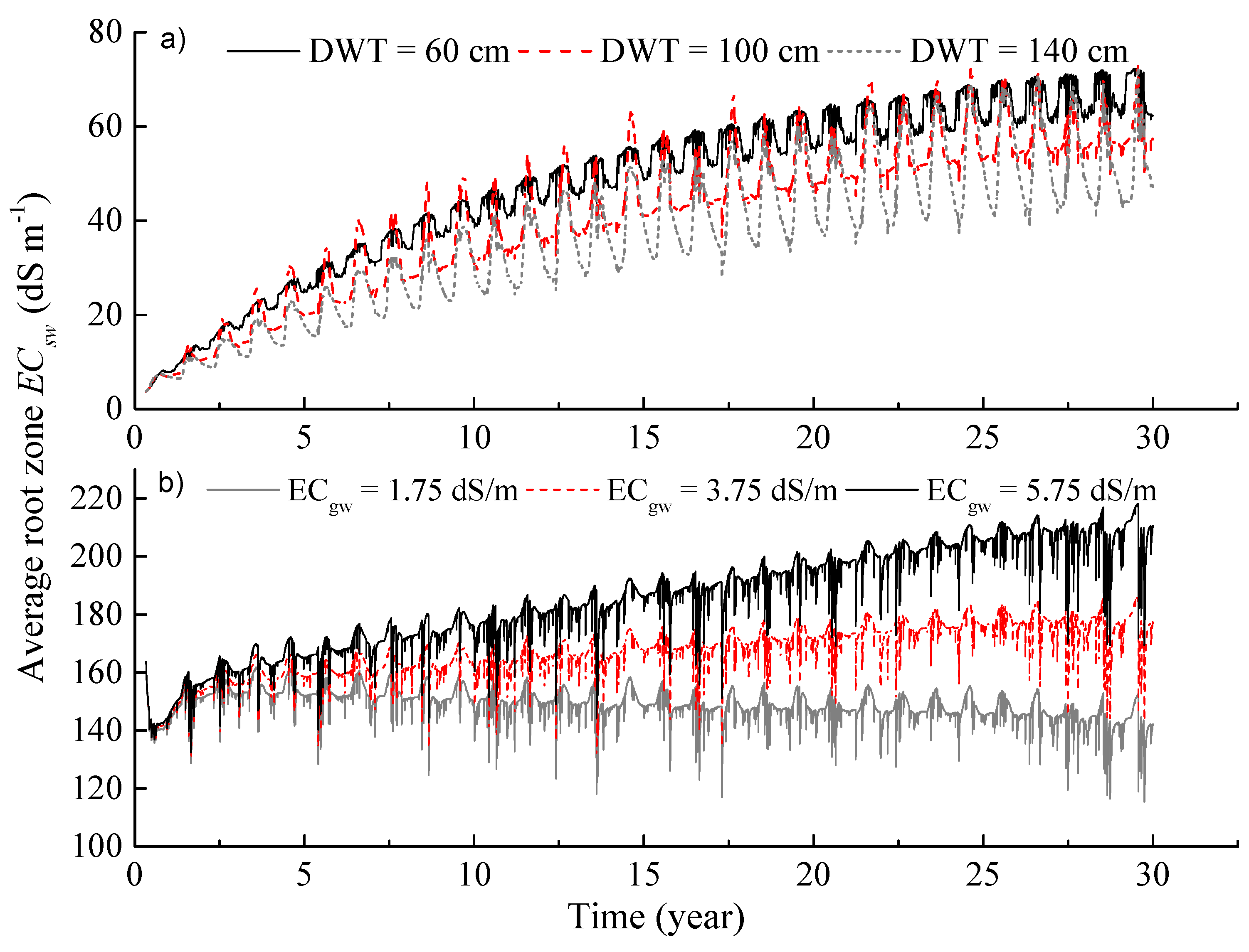
3.3.2. The Long-Term Salinization Trends

To assess long-term salinity trends, Hydrus-1D was combined with a stochastic weather generator LARS-WG to evaluate the long term changes of soil salinity under different water tables and EC_gw. Figure 7a illustrates that soil salinization increased year by year with a saline shallow ground water (EC_gw = 3.75 dS·m⁻¹). In general, root zone EC_sw increased with the upward movement of water table whereas the amplitude of the EC_sw decreased with the elevation of the water table. Average root zone EC_sw after 30 years were 62.30, 57.34 and 47.15 dS·m⁻¹ when DWT was at a depth of 60, 80 and 100 cm, respectively. These results indicated that a shallow water table contributed to increased soil salinization although the same conditions promoted root water uptake. Ibrakhimov et al. [55] found that elevated groundwater levels resulted in increased soil salinization by the annual addition of 3.5–14 t/haof salts depending on groundwater salinity. Xie et al. [4] reported that there is a contradiction between available water, salt stress, and reed water uptake with variations in DWT. Similarly, root zone EC_sw increased with the increased EC_gw, values of 142.08, 177.53, and 210.55 dS·m⁻¹ when accompanying EC_gw values were 1.75, 3.75, and 5.75 ds·m⁻¹ after 30 years, respectively (Figure 7b). The results indicated that soil salinization conditions will deteriorate continuously without human intervention and highlighted the importance of preventing human induced EC_gw increases that would occur from subsurface irrigation drainage from farmland.

Figure 7. Temporal changes in soil salinity in averaged root zone as affected by (a) water table and (b) groundwater electrical conductivity.

Figure 7. Temporal changes in soil salinity in averaged root zone as affected by (a) water table and (b) groundwater electrical conductivity.

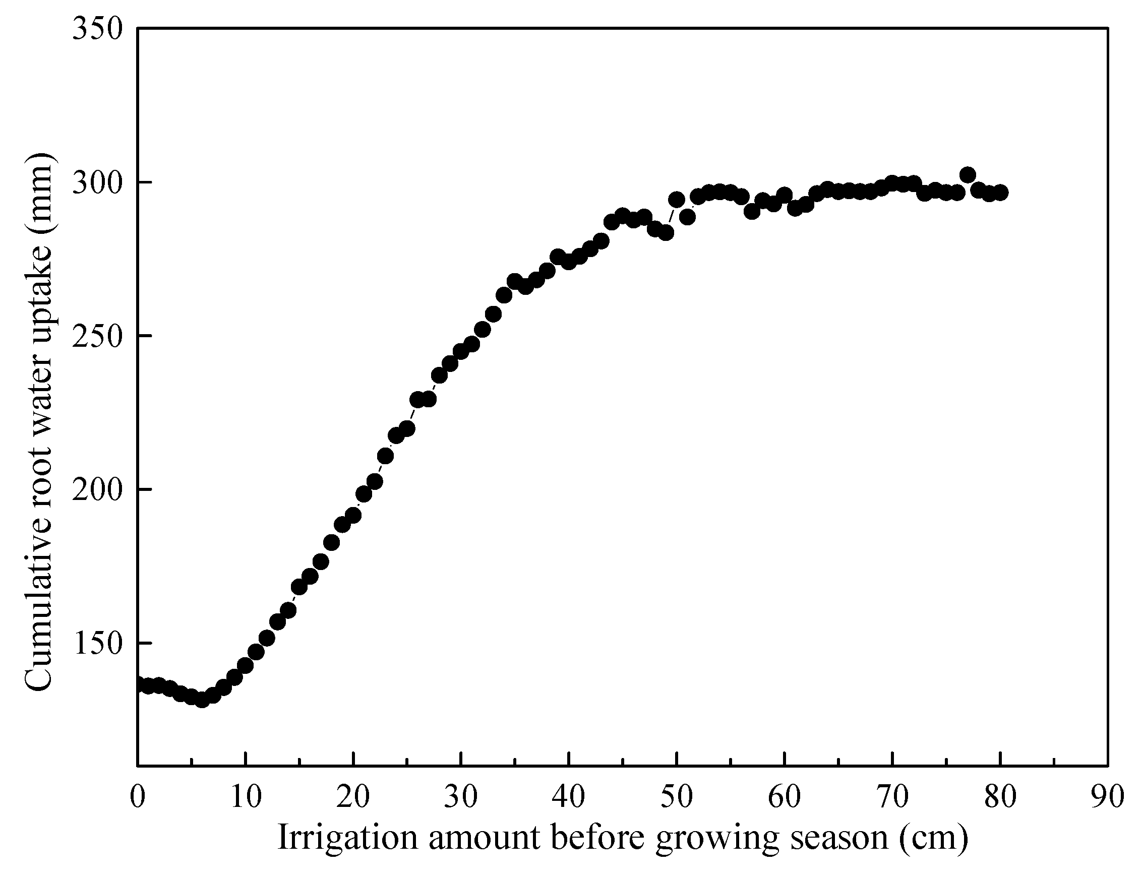
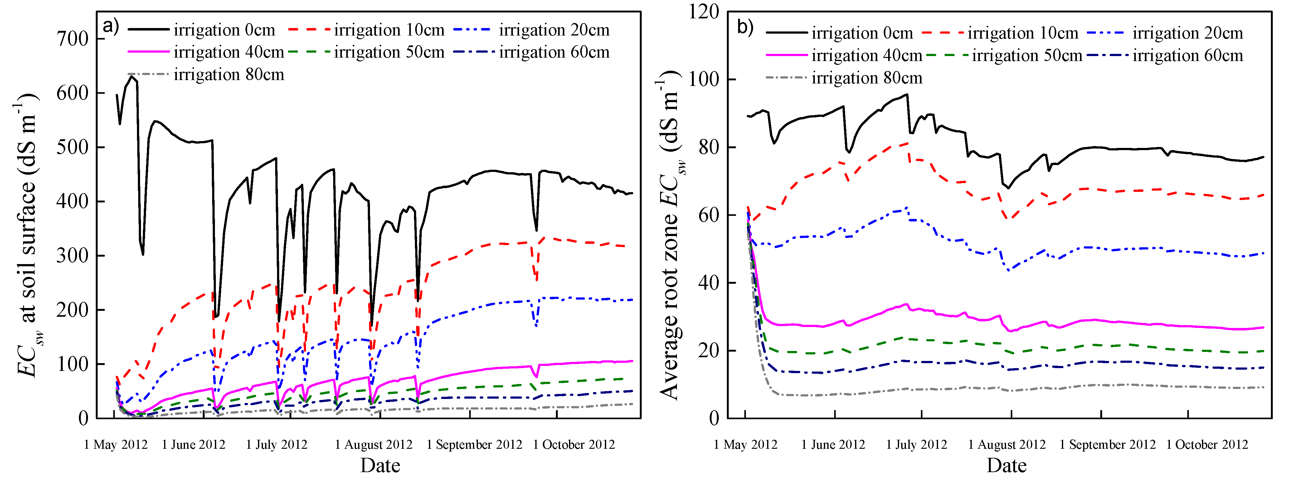
3.3.3. Preseason Irrigation Strategy

Preseason irrigation increased root water uptake significantly. Compared with no irrigation, root water uptake increased 4.5%, 40.2%, 79.3%, 100.6% and 115.4% when the irrigation amounts were 10, 20, 30, 40 and 50 cm, respectively (Figure 8). These results indicated that root water uptake generally increased with increased irrigation quantities when irrigation amounts ranged from 10 to 50 cm. However, root water uptake increased only 2 mm (from 294 to 296 mm) when the irrigation quantities increased from 50 to 80 cm, and demonstrated that irrigation quantities less than 50 cm were sufficient to promote tamarisk root water uptake (Figure 9b). Note that cumulative root water uptake displayed a decreased trend when the irrigation quantities were less than 6 cm and indicated that although a small quantity of irrigation increased the root zone water content to some extent, it was not sufficient for the salt to be effectively leached out of the root zone. Furthermore, the irrigated water cannot be easily used by the plant roots because of the water contained a large amount of soluble salts that were dissolved from the upper soil layer. This observation implied that the precipitation in the region is not beneficial for plants and even threatens plant growth, since single precipitation events are normally less than 6 cm. The increased root water uptake resulting from fresh water irrigation was mainly because sufficient quantities of water from the upper boundary layers can leach salts below the root zone and effectively alleviate salt stress (Figure 9b). Because these salts can re-accumulate as a result of evaporation (Figure 9a), repeated irrigation is needed. The average root zone EC_sw dropped rapidly below 52.5, 27.7, and 13.7 dS·m⁻¹ in 15 days when the irrigation quantities were 20, 40, and 60 cm, respectively. Therefore, irrigation before the growing season is essential, but too small or too large a quantity of irrigation is not advisable. In our case, 30–40 cm of preseason irrigation was reasonable.

Figure 8. Cumulative root water uptake of Chinese tamarisk with different irrigation amounts.

Figure 8. Cumulative root water uptake of Chinese tamarisk with different irrigation amounts.

Figure 9. Temporal changes of soil salinity at the soil surface (a) and the averaged root zone electrical conductivity as affected by irrigation amount (b).

Figure 9. Temporal changes of soil salinity at the soil surface (a) and the averaged root zone electrical conductivity as affected by irrigation amount (b).

The advantages of artificial irrigation to maintain plant growth has also been addressed by other researchers. Holland et al. [56] observed that a two-fold to five-fold increase in plant water potential and a three-fold to six-fold increase in Eucalyptus camaldulensis water consumption in three to four months after watering in the riparian region. Xie et al. [4] reported that irrigation clearly increased reed water use, especially when irrigation quantities were higher than 3 cm·d⁻¹. Askri et al. [57] demonstrated that in order to increase date palm water use, high irrigation frequencies and shallow groundwater are needed to maintain high water content and low salinity in the root zone. Therefore, we would suggest it would be beneficial to have artificial irrigation to maintain the sustainable development of the arid riparian wetlands.

4. Conclusions

In this study, soil water and salt dynamics and their effects on Tamarisk root water uptake were characterized by coupling measured data with simulation scenarios in the Heihe riparian wetland, China. The Hydrus-1D model simulations of soil water and salt dynamics matched the observed data fairly well during both the calibration and validation periods as indicated by smaller RMSE and higher R² values, which demonstrated the feasibility of using the model under different simulation scenarios.

Chinese tamarisk extends its root system into the most suitable strata with 73.6% of the total root system distributed in the 20–60 cm soil layer because of the long-term effects of water and salt stress. Groundwater is the main water source for Chinese tamarisk in the study area. Cumulative root water uptake only accounted for 41.6% of the potential value under the joint influences of water and salt stress. This result indicated the necessity of human interventions to alleviate water and salt stress. Furthermore, root water uptake was most sensitive to the fluctuations of water table levels. Too deep or too shallow a groundwater table was found to severely repress root water uptake. Shallow groundwater was found to result in increased soil salinization, especially when the groundwater contains a large amount of salts (high EC_sw). Preseason irrigation has the potential to leach salt out of the root zone and maintain the EC_sw at a reduced level during the growing season which would result in increased water uptake. Cumulative root water uptake increased when irrigation quantities were initially increased. Further increases in irrigation quantities diminished the increased rate of root water uptake.

Irrigation before the growing season is necessary, but the irrigation quantities should be taken into consideration. This study provided insights into soil water and salt redistribution and their effects on plant water use, and should help in the establishment of improved management practices for arid riparian wetlands.

References

1. Jolly, I.D.; McEwan, K.L.; Holland, K.L. A review of groundwater-surface water interactions in arid/semi-arid wetlands and the consequences of salinity for wetland ecology. Ecohydrology 2008, 1, 43–58. [Google Scholar] [CrossRef]
2. Niu, Y.; Liu, X.D.; Zhang, H.B.; Meng, H.J. The ecological function evaluation of wetland in upper and middle reaches of heihe basin. Wetl. Sci. 2007, 3, 215–220. (In Chinese) [Google Scholar]
3. Lei, K.; Zhang, M.X. The wetland resources in china and the conservation advices. Wetl. Sci. 2005, 3, 81–86. (In Chinese) [Google Scholar]
4. Xie, T.; Liu, X.; Sun, T. The effects of groundwater table and flood irrigation strategies on soil water and salt dynamics and reed water use in the yellow river delta, china. Ecol. Model. 2011, 222, 241–252. [Google Scholar] [CrossRef]
5. Ahmad, M.U.D.; Bastiaanssen, W.G.M.; Feddes, R.A. Sustainable use of groundwater for irrigation: A numerical analysis of the subsoil water fluxes. Irrig. Drain. 2002, 51, 227–241. [Google Scholar] [CrossRef]
6. Gowing, J.W.; Rose, D.A.; Ghamarnia, H. The effect of salinity on water productivity of wheat under deficit irrigation above shallow groundwater. Agric. Water Manag. 2009, 96, 517–524. [Google Scholar] [CrossRef]
7. Jiang, P.H.; Zhao, R.F.; Zhao, H.L.; Lu, L.P.; Xie, Z.L. Relationships of wetland landscape fragmentation with climate change in middle reaches of heihe river, China. J. Appl. Ecol. 2013, 24, 1661–1668. (In Chinese) [Google Scholar]
8. Zhang, H.B.; Meng, H.J.; Liu, X.D.; Zhao, W.J.; Wang, X.P. Vegetation characteristics and ecological restoration technology of typical degradation wetlands in the middle of heihe river basin, zhangye city of gansu province. Wetl. Sci. 2012, 10, 194–199. (In Chinese) [Google Scholar]
9. Feng, Q.; Liu, W.; Su, Y.H.; Zhang, Y.W.; Si, J.H. Distribution and evolution of water chemistry in heihe river basin. Environ. Geol. 2004, 45, 947–956. [Google Scholar] [CrossRef]
10. Tedeschi, A.; Dell’Aquila, R. Effects of irrigation with saline waters, at different concentrations, on soil physical and chemical characteristics. Agric. Water Manag. 2005, 77, 308–322. [Google Scholar] [CrossRef]
11. Ayars, J.E.; Shouse, P.; Lesch, S.M. In situ use of groundwater by alfalfa. Agric. Water Manag. 2009, 96, 1579–1586. [Google Scholar] [CrossRef]
12. Ayars, J.E.; Christen, E.W.; Soppe, R.W.; Meyer, W.S. The resource potential of in-situ shallow ground water use in irrigated agriculture: A review. Irrig. Sci. 2005, 24, 147–160. [Google Scholar] [CrossRef]
13. Singh, R.; Singh, J. Irrigation planning in cotton through simulation modeling. Irrig. Sci. 1996, 17, 31–36. [Google Scholar] [CrossRef]
14. Feddes, R.A.; Kabat, P.; van Bakel, P.; Bronswijk, J.J.B.; Halbertsma, J. Modelling soil water dynamics in the unsaturated zone—State of the art. J. Hydrol. 1988, 100, 69–111. [Google Scholar] [CrossRef]
15. de Jong, R.; Bootsma, A. Review of recent developments in soil water simulation models. Can. J. Soil Sci. 1996, 76, 263–273. [Google Scholar] [CrossRef]
16. Saito, H.; Šimůnek, J.; Mohanty, B.P. Numerical analysis of coupled water, vapor, and heat transport in the vadose zone. Vadose Zone J. 2006, 5, 784–800. [Google Scholar] [CrossRef]
17. Jacques, D.; Šimůnek, J.; Timmerman, A.; Feyen, J. Calibration of richards’ and convection-dispersion equations to field-scale water flow and solute transport under rainfall conditions. J. Hydrol. 2002, 259, 15–31. [Google Scholar] [CrossRef]
18. Wang, T.; Franz, T.E.; Zlotnik, V.A. Controls of soil hydraulic characteristics on modeling groundwater recharge under different climatic conditions. J. Hydrol. 2015, 521, 470–481. [Google Scholar] [CrossRef]
19. Van Genuchten, M.T. A closed-form equation for predicting the hydraulic conductivity of unsaturated soils. Soil Sci. Soc. Am. J. 1980, 44, 892–898. [Google Scholar] [CrossRef]
20. Mualem, Y. A new model for predicting the hydraulic conductivity of unsaturated porous media. Water Resour. Res. 1976, 12, 513–522. [Google Scholar] [CrossRef]
21. Šimůnek, J.; van Genuchten, M.T.; Šejna, M. Hydrus: Model use, calibration, and validation. Tansac Asabe 2012, 55, 1261–1274. [Google Scholar]
22. Šimůnek, J.; van Genuchten, M.T.; Sejna, M. The hydrus-1d software package for simulating the one-dimensional movement of water, heat, and multiple solutes in variably-saturated media. Univ. Calif. -Riverside Res. Rep. 2005, 3, 1–240. [Google Scholar]
23. Zhao, W.; Liu, B.; Zhang, Z. Water requirements of maize in the middle heihe river basin, china. Agric. Water Manag. 2010, 97, 215–223. [Google Scholar] [CrossRef]
24. Gee, G.W.; Or, D. 2.4 particle-size analysis. Methods Soil Anal. Part 2002, 4, 255–293. [Google Scholar]
25. Klute, A.; Dirksen, C. Hydraulic conductivity and diffusivity: Laboratory methods. In Methods of Soil Analysis: Part 1—Physical and Mineralogical Methods; American Society of Agronomy: Madison, WI, USA, 1986; pp. 687–734. [Google Scholar]
26. Feddes, R.A.; Kowalik, P.J.; Zaradny, H.X. Simulation of Field Water Use and Crop Yield; Centre for Agricultural Publishing and Documentation: Wageningen, The Netherlands, 1978. [Google Scholar]
27. Šimůnek, J.; Hopmans, J.W. Modeling compensated root water and nutrient uptake. Ecol. Model. 2009, 220, 505–521. [Google Scholar] [CrossRef]
28. Van Genuchten, M.T. A Numerical Model for Water and Solute Movement in and below the Root Zone; United States Department of Agriculture Agricultural Research Service U.S. Salinity Laboratory: Riverside, CA, USA, 1987.
29. Slavich, P.G.; Petterson, G.H. Estimating the electrical conductivity of saturated paste extracts from 1: 5 soil, water suspensions and texture. Soil Res. 1993, 31, 73–81. [Google Scholar] [CrossRef]
30. Corwin, D.L.; Lesch, S.M. Application of soil electrical conductivity to precision agriculture. Agron. J. 2003, 95, 455–471. [Google Scholar] [CrossRef]
31. Richards, L.A. U.S. salinity laboratory staff. In USDA Handbook No. 60. Diagnosis and Improvement of Saline and Alkali Soils; USDA: Washington, DC, USA, 1954; p. 13. [Google Scholar]
32. Allen, R.G.; Pereira, L.S.; Raes, D.; Smith, M. Crop Evapotranspiration-Guidelines for Computing Crop Water Requirements-FAO Irrigation and Drainage Paper 56; FAO: Rome, Italy, 1998; Volume 300, p. 6541. [Google Scholar]
33. Allen, R.G.; Pereira, L.S. Estimating crop coefficients from fraction of ground cover and height. Irrig. Sci. 2009, 28, 17–34. [Google Scholar] [CrossRef]
34. Schaap, M.G.; Leij, F.J.; van Genuchten, M.T. Rosetta: A computer program for estimating soil hydraulic parameters with hierarchical pedotransfer functions. J. Hydrol. 2001, 251, 163–176. [Google Scholar] [CrossRef]
35. Vanderborght, J.; Vereecken, H. Review of dispersivities for transport modeling in soils. Vadose Zone J. 2007, 6, 29–52. [Google Scholar] [CrossRef]
36. Gelhar, L.W.; Welty, C.; Rehfeldt, R.K. A critical review of data on field-scale dispersion in aquifers. Water Resour. Res. 1992, 28, 1955–1974. [Google Scholar] [CrossRef]
37. Moayyad, B. Importance of Groundwater Depth, Soil Texture and Rooting Depth on Arid Riparian Evapotranspiration; New Mexico Institute of Mining and Technology: Socorro, NM, USA, 2001. [Google Scholar]
38. Grinevskii, S.O. Modeling root water uptake when calculating unsaturated flow in the vadose zone and groundwater recharge. Mosc. Univ. Geol. Bull. 2011, 66, 189–201. [Google Scholar] [CrossRef]
39. Marquardt, D.W. An algorithm for least-squares estimation of nonlinear parameters. J. Soc. Ind. Appl. Math. 1963, 11, 431–441. [Google Scholar] [CrossRef]
40. Semenov, M.A.; Barrow, E.M.; Lars-Wg, A. A Stochastic Weather Generator for Use in Climate Impact Studies; User Manual: Hertfordshire, UK, 2002. [Google Scholar]
41. Kandelous, M.M.; Kamai, T.; Vrugt, J.A.; Šimůnek, J.; Hanson, B.; Hopmans, J.W. Evaluation of subsurface drip irrigation design and management parameters for alfalfa. Agric. Water Manag. 2012, 109, 81–93. [Google Scholar] [CrossRef]
42. Ramos, T.B.; Šimůnek, J.; Gonçalves, M.C.; Martins, J.C.; Prazeres, A.; Pereira, L.S. Two-dimensional modeling of water and nitrogen fate from sweet sorghum irrigated with fresh and blended saline waters. Agric. Water Manag. 2012, 111, 87–104. [Google Scholar] [CrossRef]
43. Siyal, A.A.; Bristow, K.L.; Šimůnek, J. Minimizing nitrogen leaching from furrow irrigation through novel fertilizer placement and soil surface management strategies. Agric. Water Manag. 2012, 115, 242–251. [Google Scholar] [CrossRef]
44. Garg, K.K.; Das, B.S.; Safeeq, M.; Bhadoria, P.B.S. Measurement and modeling of soil water regime in a lowland paddy field showing preferential transport. Agric. Water Manag. 2009, 96, 1705–1714. [Google Scholar] [CrossRef]
45. Patil, M.D.; Das, B.S.; Bhadoria, P.B.S. A simple bund plugging technique for improving water productivity in wetland rice. Soil Tillage Res. 2011, 112, 66–75. [Google Scholar] [CrossRef]
46. Vazifedoust, M.; van Dam, J.C.; Feddes, R.A.; Feizi, M. Increasing water productivity of irrigated crops under limited water supply at field scale. Agric. Water Manag. 2008, 95, 89–102. [Google Scholar] [CrossRef]
47. Robarge, W.P. Precipitation/Dissolution Reactions in Soils; CRC Press: Boca Raton, FL, USA, 1999; p. 2. [Google Scholar]
48. Herczeg, A.L.; Dogramaci, S.S.; Leaney, F.W.J. Origin of dissolved salts in a large, semi-arid groundwater system: Murray basin, australia. Mar. Freshw. Res. 2001, 52, 41–52. [Google Scholar] [CrossRef]
49. Li, C.; Lei, J.; Zhao, Y.; Xu, X.; Li, S. Effect of saline water irrigation on soil development and plant growth in the taklimakan desert highway shelterbelt. Soil Tillage Res. 2015, 146, 99–107. [Google Scholar] [CrossRef]
50. Morris, J.D.; Collopy, J.J. Water use and salt accumulation by Eucalyptus camaldulensis and Casuarina cunninghamiana on a site with shallow saline groundwater. Agric. Water Manag. 1999, 39, 205–227. [Google Scholar] [CrossRef]
51. Satchithanantham, S.; Krahn, V.; Sri Ranjan, R.; Sager, S. Shallow groundwater uptake and irrigation water redistribution within the potato root zone. Agric. Water Manag. 2014, 132, 101–110. [Google Scholar] [CrossRef]
52. Bastias, E.; Alcaraz-Lopez, C.; Bonilla, I.; Martinez-Ballesta, M.C.; Bolanos, L.; Carvajal, M. Interactions between salinity and boron toxicity in tomato plants involve apoplastic calcium. J. Plant Physiol. 2010, 167, 54–60. [Google Scholar] [CrossRef] [PubMed]
53. Brotherson, J.D.; Field, D. Tamarix: Impacts of a successful weed. Ra ngelands 1987, 9, 110–112. [Google Scholar]
54. Sala, A.; Smith, S.D.; Devitt, D.A. Water use by tamarix ramosissima and associated phreatophytes in a mojave desert floodplain. Ecol. Appl. 1996, 888–898. [Google Scholar] [CrossRef]
55. Ibrakhimov, M.; Khamzina, A.; Forkutsa, I.; Paluasheva, G.; Lamers, J.P.A.; Tischbein, B.; Vlek, P.L.G.; Martius, C. Groundwater table and salinity: Spatial and temporal distribution and influence on soil salinization in khorezm region (uzbekistan, aral sea basin). Irrig. Drain. Syst. 2007, 21, 219–236. [Google Scholar] [CrossRef]
56. Holland, K.L.; Charles, A.H.; Jolly, I.D.; Overton, I.C.; Gehrig, S.; Simmons, C.T. Effectiveness of artificial watering of a semi-arid saline wetland for managing riparian vegetation health. Hydrol. Process. 2009, 23, 3474–3484. [Google Scholar] [CrossRef]
57. Askri, B.; Ahmed, A.T.; Abichou, T.; Bouhlila, R. Effects of shallow water table, salinity and frequency of irrigation water on the date palm water use. J. Hydrol. 2014, 513, 81–90. [Google Scholar] [CrossRef]