Article

The Use of an Orographic Precipitation Model to Assess the Precipitation Spatial Distribution in Lake Kinneret Watershed

by
Eylon Shamir
1,*,
Alon Rimmer
2 and
Konstantine P. Georgakakos
1,3
1
Hydrologic Research Center, San Diego, CA 92127, USA
2
Israel Oceanographic & Limnological Research, the Kinneret Limnological Laboratory, Migdal 14950, Israel
3
Scripps Institution of Oceanography, University of California, San Diego, La Jolla, CA 92093, USA
*
Author to whom correspondence should be addressed.
Water 2016, 8(12), 591; https://doi.org/10.3390/w8120591
Submission received: 4 October 2016 / Revised: 6 December 2016 / Accepted: 6 December 2016 / Published: 13 December 2016

Abstract

:
A high-resolution 3-D orographic precipitation model (OPM) forced by Climate Forecast System (CFS) reanalysis fields was developed for the Lake Kinneret watershed (Israel-Syria-Lebanon territories). The OPM was tuned to represent the interaction between the advected and stratiform rainfall, and the local orographic enhancement. The OPM evaluation was focused on the densely instrumented lower part of the watershed. To evaluate the ungauged upper-elevation, bias-adjusted precipitation estimates from the Global-Hydro-Estimator were used. The OPM simulates higher rainfall amounts in the upper-elevation watershed compared to currently used rainfall estimates from an elevation dependent regression. The larger differences are during rain events with southwesterly wind flow and high moisture flux. These conditions, according to the OPM, are conducive to enhanced orographic lifting in the Hermon Mountain. A sensitivity analysis indicated that the higher wind speeds for southwesterly–northwesterly trajectories generate significant orographic lifting and increase the precipitation differences between the lower and upper elevations.

1. Introduction

Quantitative precipitation estimation in mountainous terrain is key for understanding the hydrologic regime in many watersheds worldwide. Precipitation estimates in these regions often rely on statistical and empirical extrapolation that associates the neighboring stations with terrain-derived characteristics, most commonly elevation, as well as other variables such as slope, aspect, and distance from the coast [1]. In mountainous terrain, however, these estimates are commonly based on in-situ observation networks with a relatively low spatial density. In addition, precipitation observations in mountainous terrain, if available, frequently carry significant uncertainty because of gauge under-catch due to strong winds, frequent snowfall events [2], and accessibility difficulties that can obstruct routine maintenance [3]. In the European Alps, for instance, a region with a relatively dense in-situ gauge network, the precipitation isohyets derived from gauge interpolation/extrapolation methods did not well reproduce the spatial variability seen in the radar images [4] and simulated by numerical models [5].
The complex topography in mountainous regions causes the perturbation and deformation of atmospheric fluxes that influence precipitation patterns by mechanically altering the wind patterns and microphysical processes, which impact condensation of the precipitable water [6]. These orographic alteration processes yield large spatial variations with, in general, enhanced precipitation in the windward side of the mountain barriers and reduced precipitation in the lee side [7].
The objective of this study is to examine the spatial variability of precipitation in mountainous terrain with scarce in-situ data. For that purpose, we used, as a diagnostic tool, a carefully constructed high-resolution Orographic Precipitation Model (hereinafter OPM). The OPM, which decouples the momentum from the energy fluxes, aims to describe the 3-D interaction of the moist wind field with the terrain in a computationally efficient manner. The OPM simulates the wind and the updraft/downdraft impact on cloud microphysical processes and the production of precipitation.
Although full physics numerical weather prediction models (such as the Weather Research and Forecasting (WRF)) are considered the state-of-the-art, there is a significant number of recent references in the scientific atmospheric sciences literature that essentially advocate the use of simplified models for diagnostic studies [8,9,10,11,12].
The OPM or other simplified models provide an attractive alternative because of the following reasons (see also [8]): (1) When applied in high resolution to a small area, the full-physics numerical models require calibration and support from observations for simulations that well represent the precipitation spatial variability [10,13,14,15,16,17]. The computational efficiency of the OPM (Section 4) allows for sensitivity analysis, generation of long time series, and ensemble simulations that preserve the deterministic signal in orographic rainfall. (2) The potential bias of the uncalibrated full-physics model in orographic applications is very significant (twice the observations mean in several cases even in the absence of strong convection), being greater than the bias of a locally calibrated OPM model [18]. (3) The development of a full-physics model with 1-km resolution over a large area and the necessary sensitivity analyses are (unfortunately) very significant computational tasks that require, in many cases, specialized computer hardware and software. These requirements may not be easily met by hydrologic groups performing local surface precipitation analysis. In such cases, the OPM approach (or other similar approaches) provides a practical alternative that relies on a leaner computational infrastructure.
The study was conducted in the Lake Kinneret watershed (Figure 1), which is comprised of a dense gauge network in its lower elevations and a sparse gauge network in the upper elevations. In this study region, the sparsely gauged upper elevation region, which constitutes about 25% of the watershed drainage area, contributes about 70% of the inflow into Lake Kinneret [19]. Clearly, a better understanding of the precipitation distribution in the watershed’s upper elevations has essential implications for water resources management and planning.
Following the literature review section of the synoptic conditions and precipitation characteristics in the Lake Kinneret watershed and the Eastern Mediterranean we describe the study area and the datasets that were used. We then describe the OPM and its implementation and configuration for the study region. The OPM simulations, which are forced by the Climate Forecast System (CFSv2) reanalysis dataset, available from the National Centers of Environmental Prediction (NCEP), were compared with observed precipitation from 90 in-situ gauges and rainfall estimates from geo-stationary satellites. Analysis of the simulated spatial precipitation distribution and the sensitivity of the precipitation distribution to various meteorological conditions is discussed and explored, preceding a section of conclusions and prospect.

2. Literature Review

2.1. Rainfall over North Israel

The predominant (~90%) large-scale (November–March) synoptic system that triggers rainfall in the eastern Mediterranean and Lake Kinneret watershed is the so-called Cyprus Low (CL) system. The CL is a mid-latitude disturbance that develops when upper trough or cut-off lows penetrate the Eastern Mediterranean [20]. These low-pressure systems are formed near Cyprus to move eastward towards the Eastern Mediterranean shore [21,22,23,24]. The passage of a CL is accompanied by westerly winds that transport moist air from Eastern Europe over the warm Mediterranean Sea where it becomes increasingly moist and conditionally unstable before it is transported over Northern Israel [25].
The rain bearing winter synoptic systems were classified by Alpert et al. (2004) [26] into seven classes based on the location of the centers along their path as related to the Island of Cyprus and the depth and pressure gradient of the cyclonic system. During the winter (January–March) CL systems commonly, have a deep upper level trough and intense vortices [27,28]. During the autumn to winter transition season (November–December) most of the events have shallow upper level trough and weak shallow vortices. The deeper systems are commonly more effective in their orographic enhancement of precipitation, and the deep cyclonic systems cause a southwesterly wind trajectory that brings significant volumes of rain into the Kinneret watershed [22].
A simpler classification of the Mediterranean rain-bearing cyclonic events is offered by [29]. Using a cluster analysis of NCEP reanalysis variables, they distinguished two type of systems, namely the shallow lows and Cyprus lows. The center of shallow low is located to the north of Israel, bringing moderate westerly winds to the Mediterranean coast. The center of the Cyprus low is above Cyprus and accompanied with a deep upper level trough to generate strong westerly winds. Most of the rain in the region is attributed to frontal and post frontal clouds that reach a minimum height of 3 km (~−5 °C), with rain clouds that often developed to be higher than 5 km (−25 °C), generating relatively cold rain [30].
Another rain-bearing synoptic system that occurs mainly during the transition seasons is the Red Sea Trough (RST), which is a low-pressure system that extends from eastern Africa through the red Sea to the Eastern Mediterranean. The RST clouds are generated over the Red Sea and carried inland by Southerly wind. Although RST storms are the leading cause of flash floods in the arid southern Israel [31], their moisture source is commonly depleted as they travel north to produce relatively weak precipitation events over Northern Israel.
The rainfall spatial distribution over the land in the eastern Mediterranean coast, in general, can be characterized as follows: (1) north–south decreasing gradient attributed to increasing distance from the main Mediterranean cyclone track; (2) west–east decreasing gradient attributed to depleted moisture further away from the Mediterranean Sea, the source of the air moisture; and (3) increase rainfall with elevation attributed to orographic enhancement [21,32,33].
Rainfall distribution over the Lake Kinneret watershed is highly variable and ranges 400–1200 mm·year−1 at the coast of the lake and the Hermon Mountain, respectively [34]. Relying on measurements from lower elevation stations, several studies found that the average monthly rainfall can be adequately described as a linear function of elevation [33,35,36,37] that is seasonally dependent [38]. In northern Israel a regression as a function of elevation tends to overestimate and underestimate observed precipitation on the windward and leeward slopes, respectively [39]. These biases are attributed to strong winds in high elevations during rainy days that cause under-catch and underestimation of rain in the gauges; wind interaction with the complex terrain that yields alternative wind pathways instead of updrafts; and impact of the enhanced rainfall that is often carried into the leeward side [39].

2.2. Atmospheric Model Studies in the Region

Several studies to simulate rainfall over the Eastern Mediterranean used atmospheric regional models that range from a simple 2-D orographic model to a fully coupled energy and momentum dynamic nested atmospheric model. A simplified 2-D orographic model was tested for the Judea Mountain Range (elevation of 400–800 m), about 100–200 km south of the study area discussed herein and oriented parallel to the coastline [40]. The Judea Mountain Range, which is affected by the same synoptic systems as the Kinneret watershed, has a strong orographic enhancement of precipitation due to horizontal wind encountering mountain slopes. Isakson (1996) [41] enhanced the model to trace the vertical displacement of the elementary volume as a function of initial position and the diabatic ascent within the lower atmospheric layer as a function of the relief.
Givati et al. (2012) [42] used a nested Weather Research and Forecast (WRF) model, forced by NCEP Global Forecast System (GFS), to simulate rainfall input for a hydrologic model that simulates streamflow in the Upper Jordan River. They reported the microphysics parameterization scheme that identifies six classes of hydrometeors and prognosis of ice, snow, and graupel as the favorable scheme during cold-cloud microphysical processes. Rostkier-Edelstein et al. (2013) [43], developed a 5-km and 2-km WRF model forced by CFS NCEP (version 1) with four-dimensional data-assimilation (FDDA) scheme, respectively. They reported that the CFS reanalysis (CFSRv1) [44] reproduced six out of the seven synoptic classes of the CL systems during the seven years that were studied [26]. Their model captured the expected impact of the synoptic condition on the rainfall intensity, generating the highest rainfall amount during deep low systems that were positioned north of Israel [22]. Both Givati et al. [42] and Rostkier-Edelstein et al. [43] experimented with the impact spatial resolution of the nested WRF model on the simulation of rainfall to conclude that high-resolution grid-spacing (1–2 km2) contributes to the understanding of the rainfall spatial distribution intricacies.
Atmospheric models were also used in several studies to dynamically downscale simulations of global climate models in order to assess the projected hydrological impact of climate change on Lake Kinneret and its watershed [45,46,47].

2.3. Orographic Precipitation Model (OPM)

The OPM used in this study was designed to simulate gridded precipitation over complex terrain in regions where orographic lifting is the key precipitation generation process. It is a simplified orographic precipitation model that decouples the momentum equation from the atmospheric moisture conservation equations, and uses a potential theory flow solution for the three-dimensional wind field over undulating terrain. This model was successfully implemented in the Sierra Nevada, Northern California [48,49,50,51,52], Southern California [53], and the Panama Canal watershed [54,55]. It was shown to perform comparably to the full-physics numerical weather prediction mesoscale models (e.g., WRF) in regions with pronounced terrain features [18,48,49,50,51,52] at a very significant computational savings.
As described above, the prevalent rainfall bearing synoptic systems in Lake Kinneret watershed are the frontal extra-tropical Mediterranean systems with strong westerly moist wind trajectories that interact with the terrain. The orographic effect in the region is not primarily driven by convective activity but rather from continuous advection of moist air through a zone of gradual topographically forced uplifting leading to prolonged duration of relatively low intensity rainfall [56]. Because of those prevalent synoptic conditions, we anticipate for a well-constructed OPM to perform well in representing the region’s precipitation spatial and temporal variability.

3. Study Area, Data and Initial Analysis

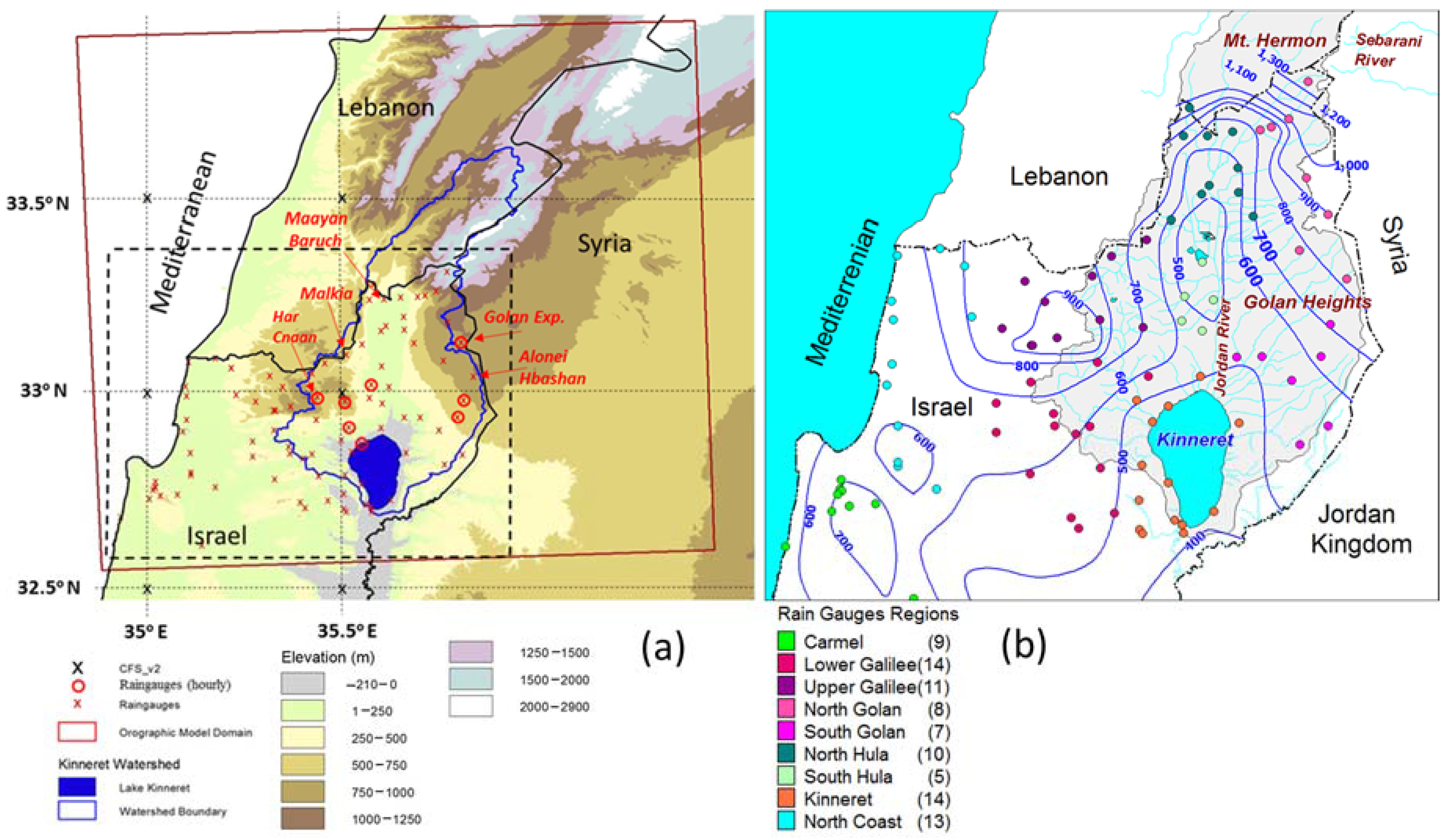
3.1. Lake Kinneret Watershed

The Lake Kinneret watershed (Figure 1) (~2570 km2, not including the area of the lake) can be broadly classified into two regions. The first region is the lower-elevation part of the watershed, which comprises the topographic drainage area of the upper Jordan River (~920 km2), and the tributaries that drain directly to lake Kinneret (965 km2). This region is predominantly within the territory of Israel, and precipitation data are routinely being collected from a dense observation network maintained by the Israeli Meteorological Service (IMS) and the Israeli Hydrological Service (IHS).
The second region consists of the higher elevation part of the watershed, which is mainly within the territory of Syria and Lebanon (~685 km2). This upper watershed contains an elongated mountain ridge (Mt. Hermon) 55-km long and 25-km wide anticline of mostly karstic limestone formation. The Hermon high elevation region receives the highest amount of precipitation in Israel (>1300 mm·year−1). Its snowpack dynamics and associated energy and mass fluxes were studied by [3], and estimates of snow cover extent and snow-water equivalent are in [57].
An average of 472 million m3 of water is contributed annually (1985–2010) to the Upper Jordan River from the karstic springs and surface flow of the Mt. Hermon region. Although Mt Hermon region makes up only 25% of the entire Kinneret watershed, its tributaries and springs contributed ~70% of the total inflow into Lake Kinneret [19]. The mismatch between the relatively small area of Mount Hermon and its large contribution of inflow to Lake Kinneret will be further examined in this study.
The aquifer underneath the Hermon is also the main source of the Awaj River in southern Syria, formed by the Sebarani and Jenani tributaries, which are fed by several karst springs along the eastern slopes of the Hermon mountain range [58], (Figure 1). The median annual discharge of the Awaj River in Syria declined to ~70 million m3 in 2004–2014 from 150 million m3 during 1982–2004 [58].

3.2. In-Situ Data

Historic quality-controlled daily rainfall data from 90 gauges over the watershed and the windward Mediterranean coastal region were retrieved from the on-line database of the Israeli Meteorological Service (IMS). This relatively dense network of observed rainfall is available for the Israeli territory of the OPM domain and covers the relatively low elevation southern portion of the Lake Kinneret watershed (the highest available station is at 960 m; Figure 1). Rainfall data for the study area from Lebanon and Syria were unavailable. The daily data from the 90 gauges were interpolated into the 1-km OPM domain using a mean inverse distance square weighted (IDW) interpolation procedure. This procedure is based on the assumption that the interpolated surface is influenced mostly by the adjacent observations and their influences diminish with distance from the interpolation target. Although various geostatistical precipitation interpolation procedures were examined for this region (e.g., [33,39,56]), this interpolation procedure was selected to serve as a baseline comparison to the OPM results because it relies solely on observations and does not pose presumptions regarding the mesoscale processes and terrain influence. Providing the highly dense network of the in situ gauges (average shortest distance between two adjacent gauges is 4 km), it is assumed that the IDW procedure will perform sufficiently well. For the interpolation of each grid cell, we used a minimum of 2 and a maximum 3 closest gauges that reported rain within a radius of 20 km. Thus, the interpolation was performed only for the grid cells that are within the rain gauges range of influence (interpolated area of 8409 km2). The average shortest and longest distances of the selected gauges from the interpolated grid-cells are 7 and 10 km, respectively. Precipitation data in high elevation at the southern part of Mt. Hermon have been routinely collected since 2005 however, data collection endures challenges because of extreme windy conditions, irregular cycle of snow accumulation and melt, and limited accessibility for routine maintenance of the stations [3]. Precipitation observations for Mt. Hermon are available from two meteorological stations: The upper meteorological station (35.78° E and 33.30° N; 2040 m) operated by the Israeli Hydrological Service (IHS) since March 2005; and the lower station (35.76° E and 33.31° N, 1640 m) operated by the Kinneret Limnological Laboratory (KLL) since January 2009.
Daily precipitation from the Hermon stations was compared with two IMS stations from the Northern Golan Height: Golan Experimental Station (35.80° E and 33.13° N; 940 m) and Alonei Habashan (35.83° E and 33.04° N, 960 m). A daily precipitation scatter plot of rainfall events from January 2012 to March 2014 in the Golan Experimental and Alonei Habashan shows a tight linear correspondence between these two stations (r2 = 0.88, Figure 2). However, the daily precipitation from the two stations of Mt. Hermon (also shown in Figure 2) poorly corresponds with the rainfall from Golan Experimental (r2 < 0.4).
The Hermon stations, which are expected to receive more precipitation because of their higher elevation, have shown no apparent signal to corroborate this positive proportionality between rain and elevation. In addition, it is evident from Figure 2 that during many days with reported precipitation in the Golan, no precipitation events were recorded at the two Hermon stations. This lack of correspondence between the Southern Hermon and the Northern Golan stations contradicts the tight correspondence that is known to be the case in the lower part of the Kinneret watershed [37,38]. Based on this analysis, we decided to exclude the Hermon stations from the spatial interpolation of the observed in-situ precipitation.

3.3. Global Hydro Estimator (GHE)

Hourly 4 × 4 km rainfall from geostationary weather satellites is available globally (60° S to 60° N) from NOAA National Environmental Satellite, Data and Information Service (NESDIS). The rainfall estimate is based on the Hydro Estimator algorithm that uses IR 10.7 μm measurements of brightness temperature at the cloud tops and associates them with rainfall rate. An attractive feature of the GHE precipitation product is its availability with short delay (less than 20 min), which makes it valuable for real time operational applications, such as flood warnings [59,60]. Hourly GHE precipitation data for this study are available since April 2012 (only for the last four selected events; see Table 1).
The GHE algorithm [61,62] identifies the cloud convective core from the surrounding clouds through a spatial analysis of the brightness temperature. The algorithm incorporates atmospheric variables from the operational NCEP Global Forecast System (GFS) model. The variables include indicators of atmospheric moisture, such as precipitable water (PW) and relative humidity. In addition, the GFS 850 hPa wind interaction with the topography at 10-km resolution is used to estimate the vertical components of the wind and to enhance [reduce] rainfall rates in the windward (leeward) slopes [63]. This GHE orographic correction component compromises its independency for verification of the OPM simulations. However, since the orographic correction is an ad-hoc procedure that is carried in a much coarser resolution than of the OPM and, as explained below, there are no alternative adequate satellite products for the region, we decided to use the GHE for a qualitative comparison with the OPM simulations.
Alternative satellite rainfall estimates may be the microwave-based products, which are available in coarser spatial and temporal resolution than the GHE (e.g., TRMM 3 h~27 km2, CMORPH 3 h~8 km2). These products, which are direct measurement of raindrops in the clouds, in general, are considered to be more accurate. However, in snow-covered areas they have difficulties separating the scattering and emission signature of the snow in the air from the signature of snow on the ground. In addition, for space-borne radar, the snowfall is often below the minimum detectible signal. Some of the microwave-based rainfall estimate algorithms mask the snow cover areas (e.g., CMORPH), while other reported high uncertainty in their precipitation estimates in snow covered areas and during snowfall events (e.g., TRMM). Both the TRMM and CMORPH products were assessed for this study and were found to poorly represent the spatial variability over the Kinneret Watershed.
The GHE precipitation product was further corrected for regional bias using a probability-distribution matching procedure [64]. Eight gauges with hourly rainfall measurements (Figure 1a) were identified with records that match the duration of the available GHE precipitation estimate. Cumulative distributions of the spatially averaged gauge rainfall and of the spatially averaged satellite rainfall for the matching grid cells of the GHE were calculated (Figure 3). The cumulative distributions were calculated for rainfall events that are larger than a trace and were reported simultaneously in both the gauges and their matching grid cells (~220 h events). It is evident that the original (uncorrected) satellite rainfall (GHE) consistently under estimate the regional average of gauge rainfall. For each decile, a multiplier was derived from the ratio of the decile-mean GHE and gauge values. The decile multipliers range from 1.3 to 1.9 (1.6 average). The hourly rainfall from the GHE was adjusted by multiplying each grid cell with its appropriate decile multiplier. This probability matching procedure is less prone to anomalies due to the relatively small sample of matching satellite-gauge precipitation events [64].

3.4. Climate Forecast System Version 2 (CFSv2) and Reanalysis (CFSR)

The NCEP Climate Forecast System version 2 (CFSv2; [65]) is operationally produced in real time since March 2011, and archived since January 2012. It provides four realizations four times a day of seasonal forecasts that extend up to nine months. The CFSv2 routinely simulates a global analysis fields at approximately 0.5 × 0.5 degrees and assimilates meteorological observations as they become available to produce spatially congruent initial model states for the atmosphere, ocean, land, and sea ice. Although the CFSv2 provides synoptic information, it is often too coarse to resolve the complex precipitation structure caused by orography, land surface heterogeneities, and land-water contrast of the study region (Figure 1a). The CFSv2 has higher resolution and considerably improved simulations compared to its previous version (CFSv1). These improvements include new physical, dynamical, and data assimilation procedures of the atmospheric, land surface and ocean models.
Boundary conditions for the OPM were determined from the 6-h 0.5° grid spacing CFS reanalysis data (CFSR; [44]). The CFSR is a retrospectively generated product that is as consistent as possible with the operational CFSv2. The CFSR variables that were used are temperature, specific humidity, and the U and V wind components all at 12 pressure levels (i.e., 1000, 925, 900, 850, 800, 750, 700, 600 500, 300, 200, and 50 mbar).

3.5. The Selected Rainfall Events

For the preceding analysis and the configuration of the OPM, seven large rainfall storms with average daily precipitation greater than 20 mm·day−1 were identified from January 2012 to March 2014 according to the measured precipitation in Mt. Cna’an rain gauge at the upper Galilee (Elevation 937 m a.s.l., Figure 1). The duration of each storm, the average daily rainfall at the gauge, and the maximum daily rainfall during each event and the availability of GHE data are shown in Table 1.

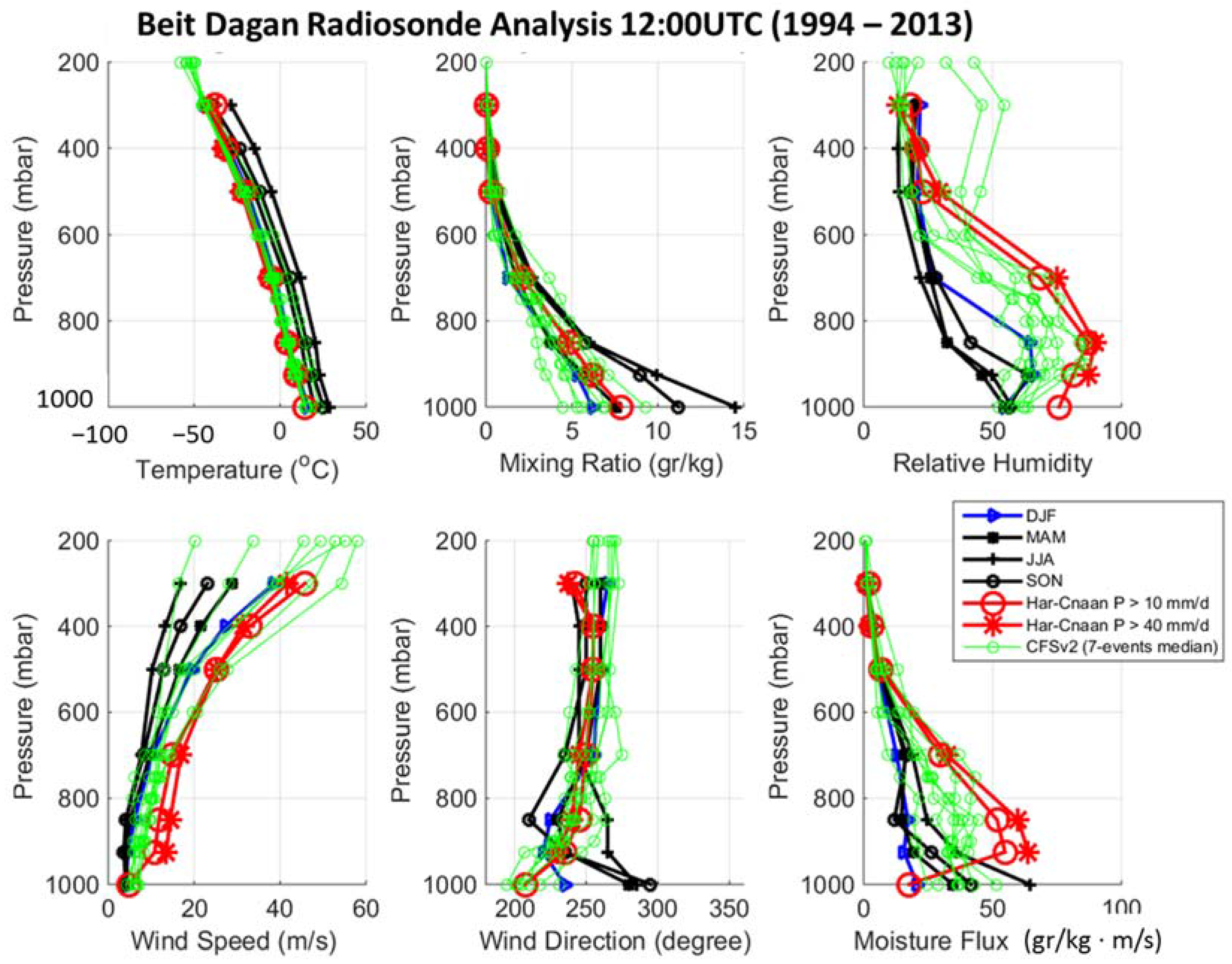
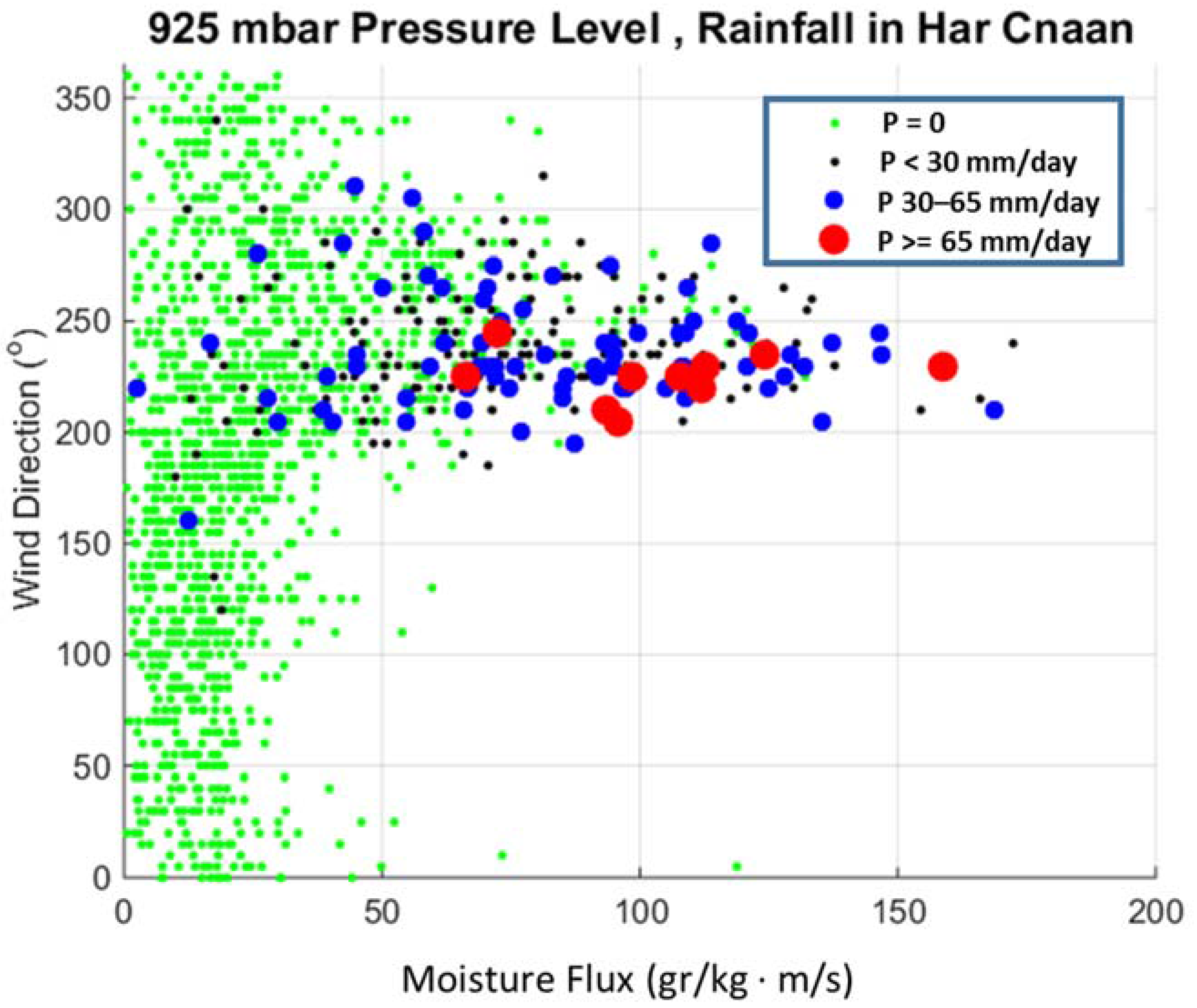
3.6. Radiosonde Analysis

Upper air sounding data from the Israeli Meteorological Service (IMS) at Beit Dagan, (about 120 km southwest of Lake Kinneret) is examined to identify sounding characteristics that are associated with rainfall over the Lake Kinneret watershed. The vertical profiles of the seasonal median of temperature (°C), mixing ratio (gr·kg−1), relative humidity (%), wind speed (m·s−1) and direction (°), and moisture flux (gr/kg·m/s); the product of the mixing ratio and the wind speed) are shown in the panels of Figure 4. The seasonal medians were calculated at 12:00 UTC for the World Meteorological Organization (WMO) mandatory reporting of pressure levels. The climatological vertical profiles for days with rainfall that exceeded 10 and 40 mm in Mt. Cna’an are indicated in red and the climatological median of the wet season (DJF) profiles are in blue. The selection of other rain gauge stations as an index yielded similar results. This is in agreement with Gur et al. (2003) [37] and Rimmer and Salingar (2006) [38] who reported that variation among rain gauges and the timing of reported maximum and minimum precipitation are similar for most stations in the Kinneret (lower) watershed.
The vertical sounding profiles of the rainy days are distinctively different than the DJF climatological values. During rainy days the temperature is consistently colder up to ~300 mbar, the mixing ratio is higher up to ~ 600 mbar, the relative humidity is much higher (up to ~500 mbar), the wind speed is faster, and the moisture flux is greater (up to 500 mbar). The prevailing wind direction during rain events is ~230 degrees in the lower atmosphere, ~250 degrees up to 400 mbar, and it shifts to 230 degrees at 300 mbar. The above-described differences from DJF climatology were larger during rain events that exceeded 40 mm·day−1. The key distinctive index during rainy days appears to be the lower level moisture flux.
The vertical sounding profiles at the 32.5N 35E grid-cell of the CFSR for the medians of the seven events are also shown in Figure 4 (green). Overall, the CFSR vertical profiles represent well the climatological sounding signal of the radiosonde during rainy days. Although a bit dryer and weaker winds than the radiosonde sounding during rain events, five of the CFSR soundings were showing the pronounced moisture flux in their lower troposphere. We note that these biases are partly because the median CFSR profiles include durations of dry spells within the events.
The skill of the CFS in predicting precipitation in the Eastern Mediterranean was assessed by [66,67] for the development of statistical downscaling procedure. Both studies however, relied on the coarse 2.5° NCEP/NOAA reanalysis for identifying the rainfall predictors and carried those relationships in order to statistically downscale the CFS (version 1). These developments although did not include a direct assessment of the CFS capacity to reproduce the rain bearing synoptic conditions over the Mediterranean, yielded reasonable reproduction of the rain characteristics over Israel. They found that the preferred predictors (30°–35° N; 30°–35° E) of rain in Northern Israel are the sea level pressure, geopotential height at 700 mbar, wind direction and velocity at 850 hPa, and the atmospheric thickness between 500 and 800 mbar. As mentioned above, the CFS adequately identified the seven CL classes [26] and was able to provide boundary conditions for mesoscale atmospheric models to yield the rainfall characteristics expected from these different CL classes [43].
The impact of the wind direction is further examined in Figure 5. The DJF 1994–2013 12:00 UTC sounding measurements at 925 hPa pressure level of moisture flux are plotted as a function of the wind direction. Days with no rain are indicated in green and three daily categories of rain are indicated with different colors and dot sizes. It is shown that rain events occurred within a narrow wind-direction band, with the largest events occurring for south–southwest wind and, during most of the large rainfall events (>65 mm·day−1), with the observed moisture flux being greater than 55 (gr/kg·m/s).

4. The Orographic Precipitation Model (OPM)

4.1. Model Structure and the Key Assumptions

The OPM formulation is available in Georgakakos (2002) [68] and Carpenter (2011) [53]. The formulation describes a set of descending and ascending air parcels that conserve vertical momentum, mass, and liquid water content. This formulation differs from earlier simplified approaches (e.g., [41,69,70]) in that it produces consistent three-dimensional velocity fields over complex terrain, and it has explicit microphysical parameterizations for the generation of cloud and precipitation. An analytical potential theory flow solution [54] provides estimates of three dimensional air velocities to produce precipitation rates over complex terrain for conditions that are non-conducive to mountain blocking [71].
The solution uses 850 hPa wind velocities from the CFSv2 reanalysis fields, and provides the boundary conditions for a three-dimensional moisture conservation model [72]. Mesoscale updrafts are generated in conditionally unstable atmospheres and the resultant precipitation is advected into the model domain. The precipitation generation component has 14 vertical levels and uses an explicit microphysical parameterization scheme for the generation of clouds and precipitation [73,74,75].
The solutions for each of 16 directions spanning 360 degrees (22.5-degree intervals) and for unit upstream wind (1 m·s−1) at 850 mbar were produced a priori in rotated coordinates. These solutions were used to provide the three dimensional wind vectors to the atmospheric moisture conservation component. For the model simulation application, the potential orographic updraft enhancement for each grid cell and for a given direction of the free wind was pre-computed for a unit magnitude of the forcing free-stream velocity and for a number of directions that cover the significant climatological wind directions. Since the potential theory flow solution is linear to the forcing wind speed magnitude, the flow velocity solutions are linearly related to the 850-mbar magnitude of the wind speed and therefore can be proportionally scaled.
The simplified solutions are valid if the following conditions are met: (1) during rain events the atmosphere is near saturation; (2) the free atmosphere has a steady uniform flow for the time interval of interest; (3) the spatial scale of the atmospheric flow fluctuations is longer than the topographic fluctuations considered; and (4) the Coriolis effect is assumed negligible for the spatial scale of interest.
Other key assumptions of the OPM are: (1) the clouds consist of condensed water that fully shares the air motion; (2) the clouds form by saturated rising air and evaporate in descending air through unsaturated environments; (3) the clouds always consist of saturated air and unsaturated air never contains clouds; (4) the clouds contain a predefined distribution of rain drop size; (5) the precipitation particles once formed are assumed to be distributed in size; (6) the precipitation drops share the horizontal motion of the air; and (7) the vertical mass transport of precipitation is based on the fall speed of the median-diameter of the precipitation particle by type (snow crystals versus raindrops).

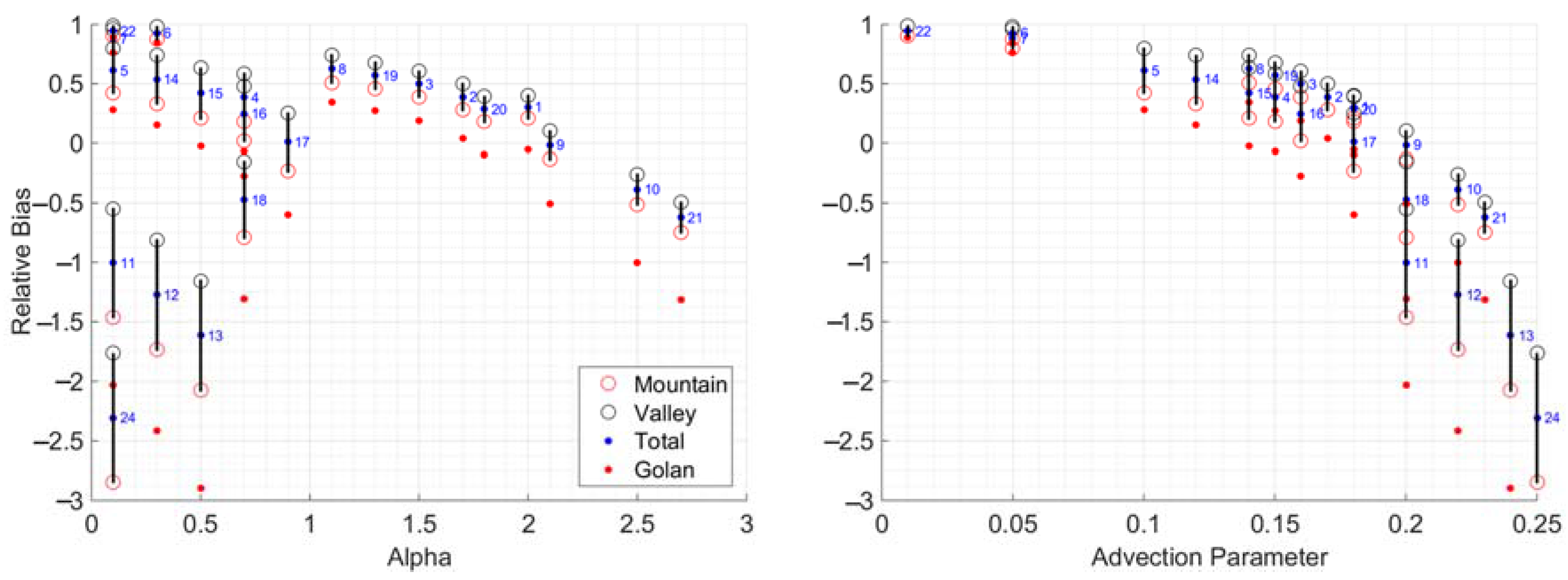
4.2. Orographic Model Set Up and Parameters Estimation

The orographic model nested domain is shown in Figure 1a (latitude 33.95°–35.56° North and Longitude 34.83°–36.44° East). The nested domain consists of 148 rows and 152 columns with 1 km grid spacing. Terrain information is based on the 90-meter digital elevation (DEM) model available from the Shuttle Radar Topography Mission, NASA, corrected with 25 m DEM from the Israeli Geological Survey mainly for the areas below sea level (0 to −210 in Figure 1a). The OPM used 6-h forcing from the upstream CFSR grid cells at 33.5N 35E and 32.5N 35E (centroids are indicated in Figure 1a).
The OPM parameters and their assigned values were tuned as described below and are shown in Table 2. The control of precipitation generation due to advection is done by tuning the RHmin925 and β parameters. The former controls the relative humidity at 925 mbar pressure level that is required to initiate updraft, and the latter is an updraft threshold value to initiate updraft in model grid cells with updraft that is lower than this threshold. Therefore, while β = 0 indicates that no rainfall will be simulated, β > 0 allows for updraft in pixels with no, or little orographic enhancement. The generation of updraft for model grid cells with no orographic lifting, enables the simulation of frontal storms as clouds are being formed at the model boundary over the Mediterranean and carried inland with onshore wind.
A manual tuning experiment was conducted to construct a model that appropriately represents the rainfall spatial distribution in the watershed (the selected parameters are listed in Table 2). Following a sensitivity analysis, we identified the two parameters α and β (Table 2) as the most sensitive parameters to control the precipitation spatial distribution. Their values balance the effect of the orographic lifting with the frontal moisture flux advection. The α has an inverse association with rainfall, which implies that smaller values of α produce more occasions of orographic lifting that result in more rain in the higher elevations. The β on the other hand, mainly controls the precipitation distribution in the lower elevations.
The densely in-situ gauged lower part of the Kinneret watershed was divided into nine distinct geo-climate regions that represent the rainfall spatial distribution: (1) Carmel Mountain; (2) Mediterranean coast; (3) Hula Valley North; (4) Hula Valley South; (5) Kinneret Coast; (6) Upper Galilee; (7) Lower Galilee; (8) Golan Height South; and (9) Golan Height North (Figure 1b). Scatter plots of the observed gauge data versus their matching OPM grid cells simulations for the seven events are shown for the different regions (Figure 6). The open circles represent the gauges while the red asterisks are for the average of the gauges over the region. The mean areal relative bias estimate of the seven storms and the correlation coefficients between the OPM and the gauges are indicated in the subplots’ upper left corner. In the current model configuration, the relatively good fit at the Golan Heights coefficients (north and south) as seen in the correlation produced an underestimation of the simulations in the lower and upper Galilee.
The relative bias B r = ( O S ) / O as a function of varying α and β is shown in Figure 7, respectively. It was calculated for each of the nine regions as the ratio between the difference of the observed rainfall (O) and the corresponding simulated rainfall (S) at the matching grid, divided by the observed rainfall at the gauges. This measure was computed using all the data for the seven events, therefore providing an aggregated spatial value for the region. Thus, negative (positive) relative bias (Br) values represent simulation over (under) estimation of the observation (notice that simulation underestimation produces measures that are bound by 1, being equal to 1 in case of 0 rain simulation).
Of particular interest is the model simulation of the Golan Heights. Since the simulations in the upper watershed could not be compared to observations from rain gauges, it is thought that in order to simulate reasonable values for the upper ungauged watershed, the processes of the Golan Heights should be well simulated. A good representation of the rainfall in the Golan indicates that the model carries the moisture flux through the Galilee Mountains barrier and produces the appropriate orographic lifting on the eastern slopes of the Hula valley reasonably well.
The blue dots in Figure 7 indicate the average relative bias within the entire model domain. The numbers in these figures are listed to indicate a specific simulation. The relative biases for the mountain regions are indicated as red open circles (i.e., Upper Galilee, Lower Galilee, Golan Height South, and Golan Height North), and for the valley regions as black open circles (i.e., Mediterranean coast, Hula Valley North, Hula Valley South and Kinneret Coast). The results for the Golan Height (i.e., Golan Height South and Golan Height North) are indicated as red dots. The black vertical lines indicate the difference between the relative bias of the mountain and valley regions.
We perceive a good simulation as one that resulted with small difference in the relative bias between the mountains and valleys.
In general, increasing α produces less rainfall and for α larger than 1 the differences in the bias between the mountain and valleys become smaller (Figure 7a). An increase in β monotonically reduces the relative bias both in mountains and valleys (Figure 7). The best results are seen for simulation #9, which has the total rainfall relative bias closer to 0 and small differences in the bias between the mountains and valleys. However, we selected simulation #2 as our preferred parametric combination (Table 2). Although it simulates a dry bias in the mountains and valleys it maintains small difference between them and it well represents the rainfall over the Golan Heights.

5. Results and Discussion

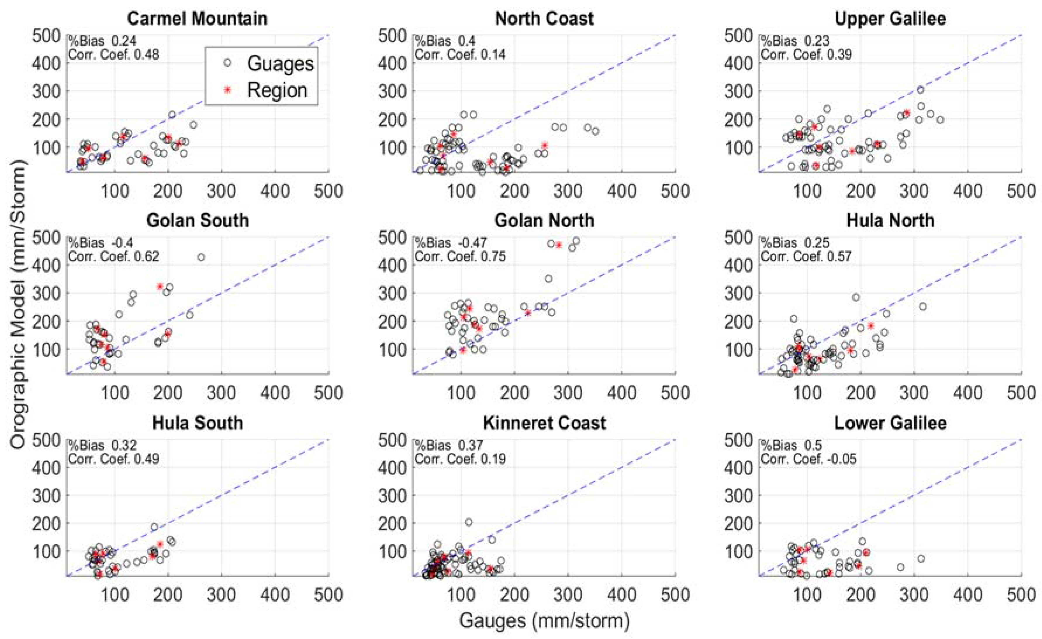
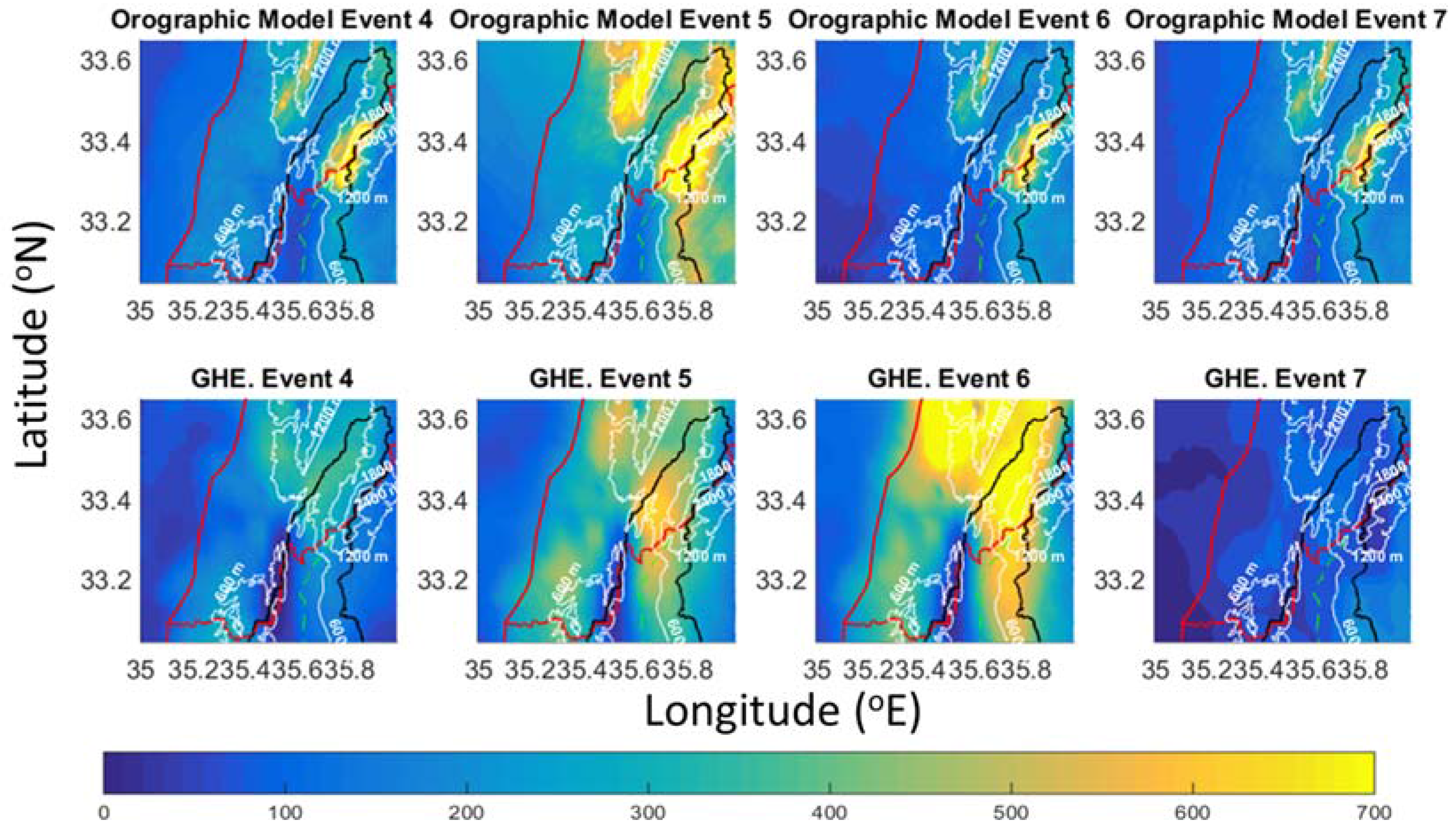
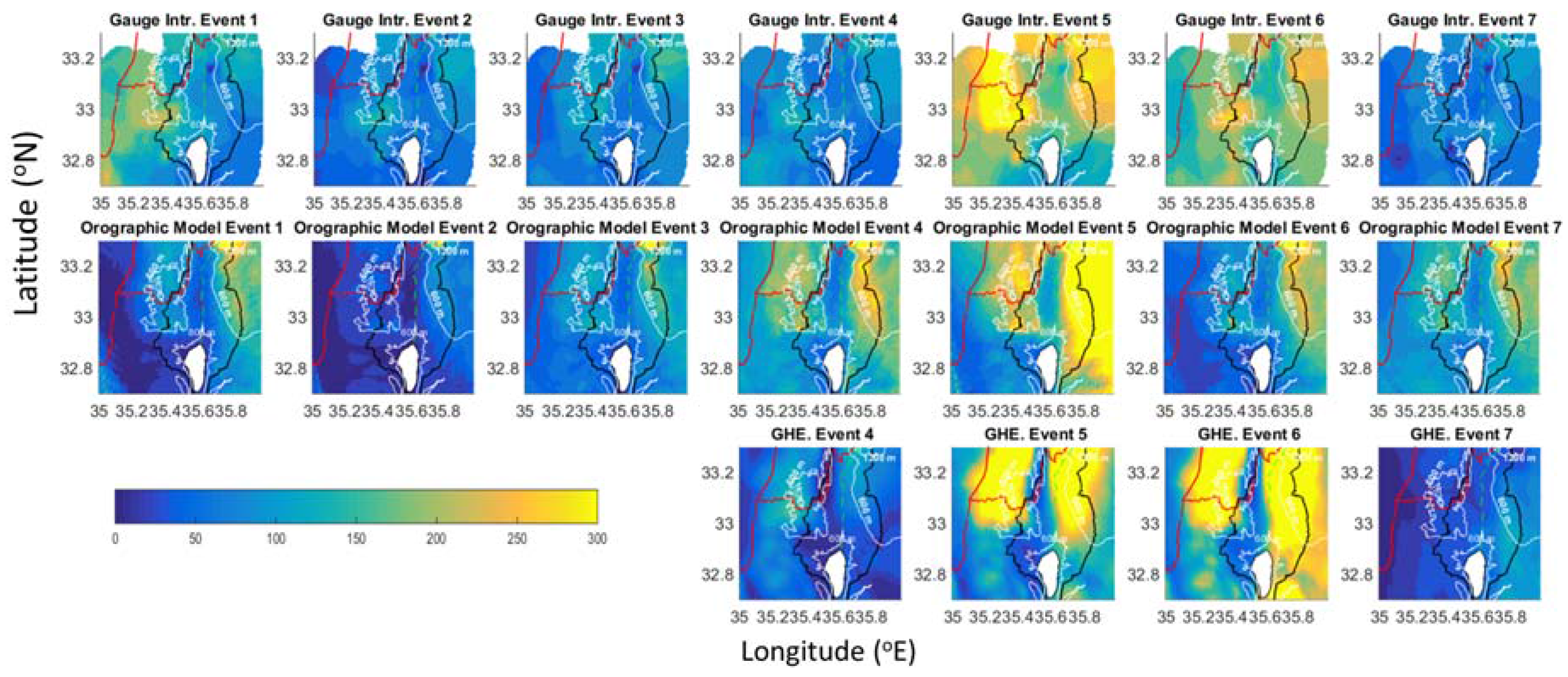
5.1. OPM Simulations Comparison with Gauge and GHE

Results of the orographic model simulation of events 1–7 (mm/event) in the lower watershed are shown in Figure 8, while the results for events 4–7 in the upper portion of the watershed are shown in Figure 9. In Figure 8, the seven panels of the upper row are the observed gauge interpolation to the models grid cells. The model simulations of the same events (middle row) are also compared with the bias corrected global hydro estimator (GHE) for events 4–7 (lower row), as mentioned above the GHE dataset in its current algorithm is only available from April 2012. Since observed gauge interpolated precipitation are absent for the upper portion of the watershed, in Figure 9 we compare the model simulations (upper row) of events 4–7 to the bias adjusted GHE (lower row). For easy interpretation, all panels have the same scale with maximum precipitation of 300 and 700 mm/event for the lower and upper watershed, respectively.
The event simulations at the lower watershed (second row in Figure 8) clearly capture the rainfall spatial distribution over the various terrain features. They show enhanced rainfall features in the western facing slopes of the upper Galilee Mountains and rainfall reduction in the eastern slopes. They also represent the lower enhancement in the Lower Galilee Mountains. The enhanced precipitation in the Golan Heights and the northern gradient is also captured fairly well by the simulations.
An interesting feature of the simulation is the dramatic increase in precipitation in the Northern upper part of the watershed at the ungagged higher elevations (Figure 9). This indicates that during CL events the slopes of the Hermon Mountains experience considerable updrafts that are likely to produce large amounts of rainfall. The GHE precipitation estimates point to a similar trend of dramatic rainfall increase during event 5 and 6. Event number 7, however, shows minimal rainfall in the high elevation but a similar enhancement pattern on the Golan Heights.
The OPM simulations of the total precipitation during the seven storm events were 2150 mm for the upper watershed and 820 mm for the lower watershed. The areal average rainfall in the upper watershed is, on average, 2.75 times (2.3–3.5 range) larger than in the lower watershed. These large ratios explain the much larger contribution of spring and streamflow from Mount Hermon to Lake Kinneret, compared to its relative surface catchment.

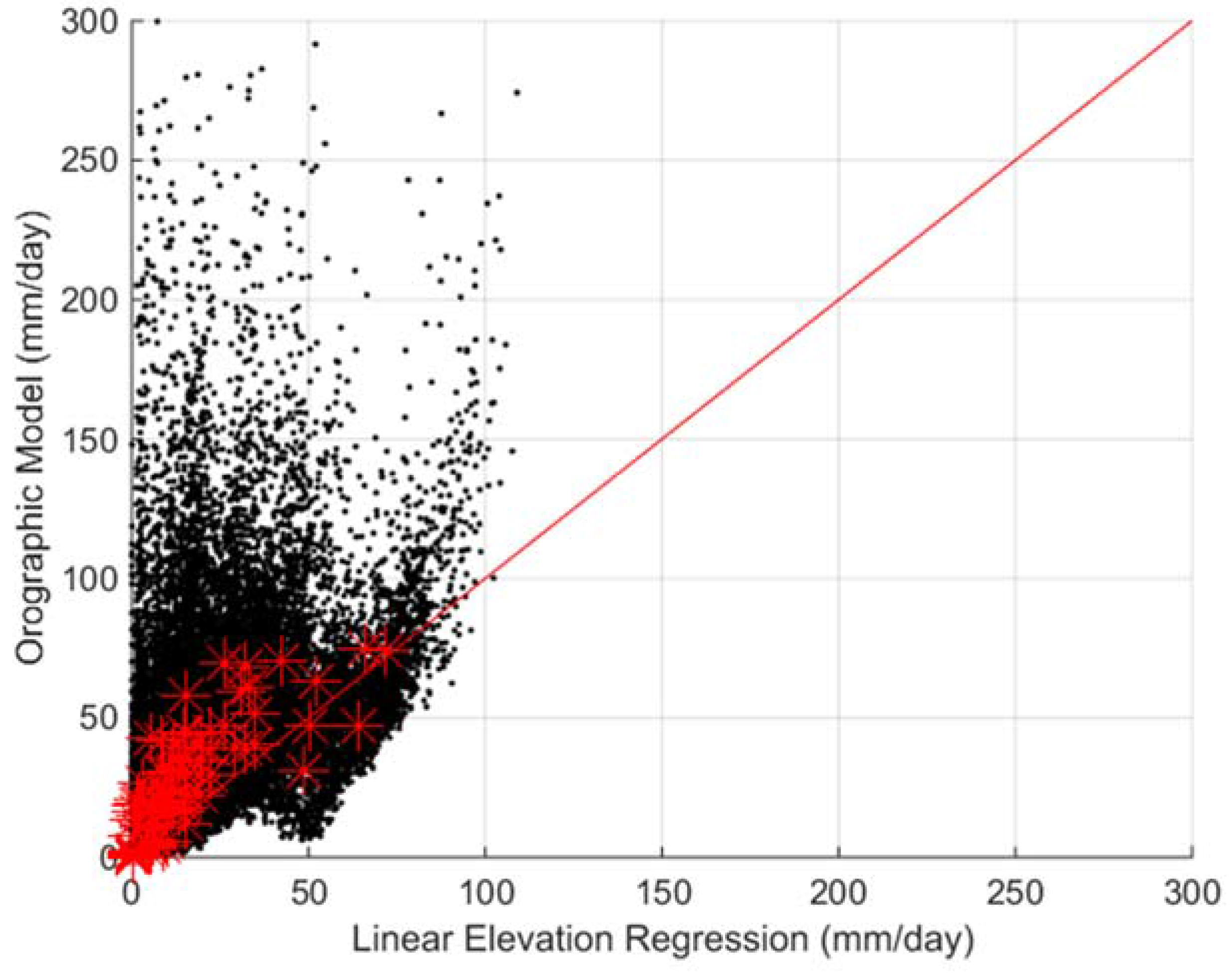
5.2. Rainfall Estimates for the Upper Watershed (Mt. Hermon)

In previous studies, the precipitation in the upper elevation watershed was extrapolated by using a linear regression with elevation. It was based on daily measured rainfall in gauges at the lower part of the watershed. In Figure 10, the daily rainfall estimates from the orographic model are compared with daily rainfall estimates from the seasonally varying linear regression developed by Rimmer and Salinger, (2006), Equations (18) and (19) [38]. The comparison in this Figure is for the fraction of the watershed that is north of 33.25° N Latitude, and includes the highest parts of Mt. Hermon (>960 m). The estimated rainfall by the regression is based on the simulated daily rainfall at the grid cells of the OPM that match with three index stations (i.e., Golan Experimental, Malkia, and Maayan Baruch, Figure 1).
The scattered black dots in Figure 10 represent daily precipitation of the 705 grid cells of the upper elevation watershed, while the red asterisks represent the mean areal daily averages during the 7 events (~50 days). The orographic model results in a wide range of simulated rainfall, attributed to the complex dynamics and geographical terrain that are accounted for in the model. On average, the orographic model simulations overestimate the regression estimates by 53% with the overestimation amount dropping for higher rainfall amounts. The differences between the mean and the standard deviation of the daily rainfall of the orographic model and the regression model are plotted as a function of the moisture flux and the wind direction in the 12:00 UTC 900 mbar from the CFSR at 32.5° N, 35.0° E (Figure 11). The larger deviation of the mean and the standard deviation (upper tercile) indicate conditions in which these two models deviate the most. The larger standard deviations and average differences occur only when the moisture flux is greater than 100 gr/kg·m/s and for southwest wind direction. These results emphasize the importance of the interaction of the mesoscale condition with the complex terrain of the Hermon Mountains. We do note that the rainfall in the model is also dependent on the evolution of the storm and the state of the atmospheric moisture (antecedent moisture conditions).
Assessing the last four events (events 4–7) that have GHE precipitation data, the ratio between the total mean areal precipitation of the upper and lower watershed for the OPM simulations, the regression estimate using the OPM simulation for the key three stations, and the GHE rainfall estimates were 2.45, 1.45 and 2.23, respectively. Note that the bias adjusted GHE ratio is very close to the OPM simulations. This provides additional support to the argument that the elevation based regression may underestimate the precipitation in the upper watershed.
The wind vertical drafts (up and down), an indicator for the orographic influence on the precipitation, are tightly dependent on the wind upstream direction. The average wind vertical drafts in the upper lake Kinneret watershed, as calculated for the 16 upstream directions (22.5 degrees intervals) using unit upstream wind (1 m·s−1) at 850 mbar, are shown in Figure 12. It is seen that upstream wind directions that experience precipitation events (180–300 degrees, see Figure 11) have a wide range of average vertical wind draft that ranges from the largest downdraft at 180 degrees to the largest updraft at 270 degrees and declining updraft as the upstream wind shifts to the north. This suggests that a slight change in upstream wind direction may substantially influence the orographic processes in the upper watershed.
Examples of the spatial distribution in the upper watershed of the wind vertical draft with four possible wind directions during CL (i.e., 180°, 225°, 270°, and 315°) are presented in Figure 13. A plot of the terrain is also added to this figure for easy reference. The patterns of the wind vertical draft are clearly very different for the different directions. Most notably are the changes in the Hermon Mountain range in the eastern portion of the watershed. In this area, the vertical wind is changing from a strong downdraft to updraft as the upstream wind direction shifts from south to north with a peak updraft for the west direction.

6. Conclusions and Prospect

An orographic precipitation model was set up at a 1-km spacing resolution for a domain that covers the watershed of Lake Kinneret in order to study the precipitation spatial distribution. The OPM is forced by the CFSR (~0.5°) and configured for seven major rainfall events (2012–2014). The model results were compared to observed gauge rainfall and the bias adjusted geo-stationary rainfall estimate from the Global Hydro Estimator available for four of the events (NESDIS/NOAA). A model was tuned to assign a combination of model parameters that favorably represent the spatial distribution in the lower (gauged) part of the watershed. The selected parameters balance the rainfall generation from orographic lifting with the advected stratiform rainfall. We note, however, that the model evaluation was carried for the lower portion of the watershed where dense rainfall observation network is available within the territory of Israel. For the upper portion of the watershed, measured in-situ precipitation data were highly uncertain, and the available precipitation data is from satellites.
Lake Kinneret receives most of its inflow from discharge of the three largest springs in the Jordan River headwater. The drainage area of these springs comprised of the basin’s higher elevation which lacks accurate in-situ precipitation observations. Precipitation for the upper watershed has been traditionally estimated using data analysis from the dense instrumental network of the lower basin. Using the OPM as a diagnostic tool, we examined the relationships between the lower and the upper watershed. It was found that the regression extrapolation underestimates the OPM simulations by more than 50%. This result suggests that representing the rainfall in the upper watershed as an aggregate that can be estimated with a simple regression might be an oversimplification.
The regression yields results that cannot represent the complexity of the rainfall distribution and the dependency on the variability of the synoptic conditions. The simulations also indicate that a major factor that determines the rainfall distribution is the wind speed and direction. An analysis of the wind vertical draft in the upper watershed indicates large differences that are dependent on the upstream wind direction. Further research should be performed on the rainfall distribution in the upper ungauged Kinneret watershed. In addition, operational quantitative precipitation estimates for the upper Lake Kinneret watershed should be extrapolated using an empirical procedure that incorporates the available in-situ precipitation observations in the lower portion of the watershed and the synoptic meteorological variables.
Additionally fruitful work would also be the use of locally calibrated full-physics models with comparable resolution for (necessarily) few selected events for the region of interest. This would help understand the impact to the surface precipitation of the simplifications made using the approach of this work, and would lead to understanding any additional factors that may control the surface precipitation distribution in the region.
Finally, the demonstrated good match of the computationally efficient OPM to the observed gauge data, in conjunction with the synoptic predictive skill of the CFSv2 [43,66], point to the potential for this modeling configuration of the OPM to serve as an efficient diagnostic and possibly predictive precipitation model for the Eastern Mediterranean in general with high resolution over large domains.

Acknowledgments

Support for this study was provided by the Technology Transfer Program of the Hydrologic Research Center, San Diego, California.

Author Contributions

All authors designed and conceived the study. Eylon Shamir performed the experiments and was the lead writer of the manuscript. Alon Rimmer assisted with data assembly and analysis in addition to interpretation of the model simulations. Konstantine P. Georgakakos developed and enhanced the Orographic Precipitation Model for the study region.

Conflicts of Interest

The authors declare no conflict of interest.

References

  1. Daly, C.; Neilson, R.P.; Phillips, D.L. A statistical-topographic model for mapping climatological precipitation over mountainous terrain. J. Appl. Meteorol. 1994, 33, 140–158. [Google Scholar] [CrossRef]
  2. Groisman, P.Y.; Legates, D.R. The accuracy of United States precipitation data. Bull. Am. Meteorol. Soc. 1994, 75, 215–227. [Google Scholar] [CrossRef]
  3. Sade, R.; Rimmer, A.; Litaor, I.M.; Shamir, E.; Furman, A. Snow surface energy and mass balance in a warm temperate climate mountain. J. Hydrol. 2014, 519, 848–862. [Google Scholar] [CrossRef]
  4. Germann, U.; Joss, J. Variograms of radar reflectivity to describe the spatial continuity of Alpine precipitation. J. Appl. Meteorol. 2001, 40, 1042–1059. [Google Scholar] [CrossRef]
  5. Zangl, G.; Aulehner, D.; Wastl, C.; Pfeiffer, A. Small-scale precipitation variability in the Alps: Climatology in comparison with semi-idealized numerical simulations. Q. J. R. Meteorol. Soc. 2008, 134, 1865–1880. [Google Scholar] [CrossRef]
  6. Wang, J.; Georgakakos, K.P. Validation and sensitivities of dynamic precipitation simulation for winter events over the Folsom Lake watershed: 1964–1999. Mon. Weather Rev. 2005, 133, 3–19. [Google Scholar] [CrossRef]
  7. Smith, R.B. The influence of mountains on the atmosphere. Adv. Geophys. 1979, 21, 87–230. [Google Scholar]
  8. Gutmann, E.; Barstad, I.; Clark, M.; Arnold, J.; Rasmussen, R. The intermediate complexity atmospheric research model (ICAR). J. Hydrometeorol. 2016, 17, 957–973. [Google Scholar] [CrossRef]
  9. Wayand, N.E.; Hamlet, A.F.; Hughes, M.; Feld, S.I.; Lundquist, J.D. Intercomparison of meteorological forcing data from empirical ad mesoscale model sources in the North Fork American River Basin in Northern Sierra Nevada, California. J. Hydrometeorol. 2013, 14, 677–699. [Google Scholar] [CrossRef]
  10. Watson, C.D.; Lane, T.P. Sensitivities of orographic precipitation to terrain geometry and upstream conditions in idealized simulations. J. Atmos. Sci. 2012, 69, 1208–1231. [Google Scholar] [CrossRef]
  11. Kunz, M. Characteristics of large-scale orographic precipitation in a linear perspective. J. Hydrometeorol. 2011, 12, 27–43. [Google Scholar] [CrossRef]
  12. Barstad, I.; Shuller, F. An extension of Smith’s linear theory of orographic precipitation; Introduction of vertical layers. J. Atmos. Sci. 2011, 68, 2695–2709. [Google Scholar] [CrossRef]
  13. Wetzel, M.; Meyers, M.; Borys, R.; McAnelly, R.; Cotton, W.; Rossi, A.; Frisbie, P.; Nadler, D.; Lowenthal, D.; Cohn, S.; et al. Mesoscale Snowfall Prediction and Verification in Mountainous Terrain. Weather Forecast. 2003, 19, 806–828. [Google Scholar] [CrossRef]
  14. Jimenez, P.A.; Dudhia, J. Improving the representation of resolved and unresolved topographic effects on surface wind in the WRF model. J. Appl. Meteorol. Clim. 2012, 51, 300–316. [Google Scholar] [CrossRef]
  15. Sindosi, O.A.; Bartzokas, A.; Kotroni, V.; Lagouvardos, K. Influence of orography on precipitation amount and distribution in NW Greece: A case study. Atmos. Res. 2015, 152, 105–122. [Google Scholar] [CrossRef]
  16. Wilson, A.M.; Barros, A.P. Landform controls on low-level moisture convergence and the diurnal cycle of warm season orographic rainfall in the Southern Appalachians. J. Hydrol. 2015, 531, 475–493. [Google Scholar] [CrossRef]
  17. Scheffknecht, P.; Richard, E.; Lambert, D. A highly localized high precipitation event over Corsica. Q. J. R. Meteorol. Soc. 2016, 142, 206–221. [Google Scholar] [CrossRef]
  18. Georgakakos, K.P.; Graham, N.E.; Modrick, T.M.; Murphy, M., Jr.; Shamir, E.; Spencer, C.; Sperfslage, J.A. Evaluation of real-time hydrometeorological ensemble prediction on hydrologic scales in Northern California. J. Hydrol. 2014, 519, 2978–3000. [Google Scholar] [CrossRef]
  19. Rimmer, A.; Givati, A. Hydrology. Chapter 7. In Lake Kinneret: Ecology and Management; Zohary, T., Sukenik, A., Berman, T., Nishri, A., Eds.; Springer: Heidelberg, Germany, 2014. [Google Scholar]
  20. Zangvil, A.; Druian, P. Upper Air Trough Axis Orientation and the Spatial-Distribution of Rainfall over Israel. Int. J. Climatol. 1990, 10, 57–62. [Google Scholar] [CrossRef]
  21. Goldreich, Y. The Climate of Israel: Observation, Research and Application; Kluwer Academic/Plenum Publishers: New York, NY, USA, 2003; p. 270. [Google Scholar]
  22. Saaroni, H.; Halfon, N.; Ziv, B.; Alpert, P.; Kutiel, H. Links between the rainfall regime in Israel and location and intensity of Cyprus lows. Int. J. Climatol. 2010, 30, 1014–1025. [Google Scholar] [CrossRef]
  23. Ziv, B.; Saaroni, H.; Romem, M.; Heifetz, E.; Harnik, N.; Baharad, A. Analysis of Conveyor Belts in Winter Mediterranean Cyclones. Theor. Appl. Climatol. 2010, 99, 441–455. [Google Scholar] [CrossRef]
  24. Lionello, P. The Climate of the Mediterranean Region, from the Past to the Future, 1st ed.; Elsevier: Amsterdam, The Netherlands, 2012. [Google Scholar]
  25. Shay-El, Y.; Alpert, P. A diagnostic study of winter diabatic heating in the Mediterranean in relation with cyclones. Q. J. R. Meteorol. Soc. 1991, 117, 715–747. [Google Scholar] [CrossRef]
  26. Alpert, P.; Osetinsky, I.; Ziv, B.; Shafir, H. Semi-objective classification for daily synoptic systems: Application to the Eastern Mediterranean climate change. Int. J. Climatol. 2014, 24, 1001–1011. [Google Scholar] [CrossRef]
  27. Goldreich, Y.; Mozes, H.; Rosenfeld, D. Radar analysis of cloud systems and their rainfall yield, in Israel. Isr. J. Earth Sci. 2004, 53, 63–76. [Google Scholar] [CrossRef]
  28. Alpert, P.; Neeman, B.U.; Shay-El, Y. Climatological analysis of Mediterranean cyclones using ECMWF data. Tellus 1990, 42, 65–77. [Google Scholar] [CrossRef]
  29. Peleg, N.; Morin, E. Convective rain cells: Radar derived spatiotemporal characteristics and synoptic patters over eastern Mediterranean. J. Geophys. Res. 2012, 117, 1–17. [Google Scholar] [CrossRef]
  30. Rosenfeld, D. Dynamic Characteristics of Cumuliform Clouds and Cloud Systems and their Influence on Rainfall. Ph.D. Thesis, Hebrew University of Jerusalem, Jerusalem, Israel, 1986. [Google Scholar]
  31. Kahana, R.; Ziv, B.; Enzel, Y.; Dayan, U. Synoptic climatology of major floods in the Negev Desert, Israel. Int. J. Climatol. 2002, 22, 867–882. [Google Scholar] [CrossRef]
  32. Katsnelson, J. The variability of annual precipitation in Palestine. Arch. Meteorol. Geophys. Bioklimatol. 1964, 13, 163–172. [Google Scholar] [CrossRef]
  33. Kutiel, H. Rainfall variations in the Galilee (Israel). I. Variations in the spatial distribution in the periods 1931–1960 and 1951–1980. J. Hydrol. 1987, 94, 331–344. [Google Scholar] [CrossRef]
  34. Ziv, B.; Shilo, E.; Rimmer, A. Meteorology. Chapter 6. In Lake Kinneret—Ecology and Management; Zohary, T., Sukenik, A., Berman, T., Nishri, A., Eds.; Springer: The Netherlands, 2014; pp. 81–97. [Google Scholar]
  35. Gilad, D.; Schwartz, S. Hydrogeology of the Jordan sources aquifers. Isr. Hydrol. Ser. Rep. Hydrol. 1978, 58, 5–78. (In Hebrew) [Google Scholar]
  36. Simpson, B.; Carmi, I. The hydrology of the Jordan tributaries (Israel) hydrographic and isotopic investigation. J. Hydrol. 1983, 62, 225–242. [Google Scholar] [CrossRef]
  37. Gur, D.; Bar-Matthews, M.; Sass, E. Hydrochemisty of the main Jordan River sources: Dan, Banias, and Kezinim springs, north Hula Valley, Israel. Isr. J. Earth Sci. 2003, 52, 155–178. [Google Scholar] [CrossRef]
  38. Rimmer, A.; Salingar, Y. Modelling precipitation-streamflow processes in Karst basin: The case of the Jordan River sources, Israel. J. Hydrol. 2006, 331, 524–542. [Google Scholar] [CrossRef]
  39. Halfon, N.; Kutiel, H. Changes in the spatial and temporal characteristics of rainfall in Northern Israel and their meaning. Horiz. Geogr. 2004, 62, 33–42. (In Hebrew) [Google Scholar]
  40. Alpert, P.; Shafir, H. A physical model to complement rainfall normal over complex terrain. J. Hydrol. 1989, 110, 51–62. [Google Scholar] [CrossRef]
  41. Isakson, A. Rainfall distribution over central and southern Israel induced by large-scale moisture flux. J. Appl. Meteorol. 1996, 35, 1063–1075. [Google Scholar] [CrossRef]
  42. Givati, A.; Lynn, B.; Liu, Y.; Rimmer, A. Coupling high-resolution WRF with a hydrological model for operational prediction of Jordan River stream flow. J Appl. Meteorol. Climatol. 2012, 51, 285–299. [Google Scholar] [CrossRef]
  43. Rostkier-Edelstein, D.; Liu, Y.; Wu, W.; Kunin, P.; Givati, A.; Ge, M. Towards a high-resolution climatography of seasonal precipitation over Israel. Int. J. Climatol. 2014, 34, 1964–1979. [Google Scholar] [CrossRef]
  44. Saha, S.; Moorthi, S.; Pan, H.L.; Wu, X.; Wang, J.; Nadiga, S.; Tripp, P.; Kistler, R.; Woollen, J.; Behringer, D.; et al. The NCEP Climate Forecast System Reanalysis. Bull. Am. Meteorol. Soc. 2010, 90, 1015–1057. [Google Scholar] [CrossRef]
  45. Rimmer, A.; Givati, A.; Samuels, R.; Alpert, P. Using ensemble of climate models to evaluate future water and solutes budgets in Lake Kinneret, Israel. J. Hydrol. 2011, 410, 248–259. [Google Scholar] [CrossRef]
  46. Smiatek, G.; Kunstmann, H.; Heckl, A. High-resolution climate change simulations for the Jordan River area. J. Geophys. Res. 2011, 116. [Google Scholar] [CrossRef]
  47. Smiatek, G.; Kunstmann, H.; Heckl, A. High-Resolution Climate Change Impact Analysis on Expected Future Water Availability in the Upper Jordan Catchment and the Middle East. J. Hydrometeorol. 2014, 15, 1517–1531. [Google Scholar] [CrossRef]
  48. Hydrologic Research Center-Georgia Water Resources Institute (HRC-GWRI). Integrated Forecast and Reservoir Management (INFORM) for Northern California: System Development and Initial Demonstration; PIER Energy-Related Environmental Research, CEC-500-2006-109, 244pp + 9 Appendices; California Energy Commission: Sacramento, CA, USA, 2007.
  49. Hydrologic Research Center-Georgia Water Resources Institute (HRC-GWRI). Implications of Climatic Changes for Northern California Water Resources Management for the Later Part of the 21st Century; PIER Energy-Related Environmental Research, Final Report, Award No. 500-07-013; California Energy Commission: Sacramento, CA, USA, 2010; p. 114.
  50. Hydrologic Research Center-Georgia Water Resources Institute (HRC-GWRI). INFORM Enhancement and Demonstration Results for Northern California (2008–2012); PIER Energy-Related Environmental Research, Publication # CEC-500-2014-019, 224pp. + 6 Appendices; California Energy Commission: Sacramento, CA, USA, 2014.
  51. Georgakakos, K.P.; Graham, N.E.; Cheng, F.Y.; Spencer, C.; Shamir, E.; Georgakakos, A.P.; Yao, H.; Kistenmacher, M. Value of adaptive water resources management in northern California under climatic variability and change: Dynamic hydroclimatology. J. Hydrol. 2012, 412, 47–65. [Google Scholar] [CrossRef]
  52. Georgakakos, A.P.; Yao, H.; Kistenmacher, M.; Georgakakos, K.P.; Graham, N.E.; Cheng, F.Y.; Spencer, C.; Shamir, E. Value of adaptive water resources management in northern California under climatic variability and change: Reservoir Management. J. Hydrol. 2012, 412, 34–46. [Google Scholar] [CrossRef]
  53. Carpenter, T. An Interdisciplinary Approach to Characterize Flash Flood Occurrence Frequency for Mountainous Southern California. Ph.D. Thesis, Scripps Institution of Oceanography, University of California, San Diego, CA, USA, 2011. [Google Scholar]
  54. Georgakakos, K.P.; Sperfslage, J.A.; Tsintikidis, D.; Carpenter, T.M.; Krajewski, W.F.; Kruger, A. Design and Tests of an Intergrated Hydrometeorological Forecast System for the Operational Estimation and Forecasting of Rainfall and Streamflow in the Mountainous Panama Canal watershed; HRC Technical Report No. 2; Hydrologic Research Center: San Diego, CA, USA, 1999. [Google Scholar]
  55. Georgakakos, K.P.; Sperfslage, J.A. Operational Rainfall and Flow Forecasting for the Panama Canal Watershed. In The Río Chagres, Panama; Harmon, R.S., Ed.; Water Science and Technology Library; Springer: Dordrecht, The Netherlands, 2005; pp. 325–335. [Google Scholar]
  56. Sharon, D.; Kutiel, H. The distribution of rainfall intensity in Israel, its regional and seasonal variation and its climatological evaluation. J. Climatol. 1986, 6, 277–291. [Google Scholar] [CrossRef]
  57. Mhawej, M.; Faour, G.; Fayad, A.; Shaban, A. Towards an enhanced method to map snow cover areas and derive snow-water equivalent in Lebanon. J. Hydrol. 2014, 513, 274–282. [Google Scholar] [CrossRef]
  58. Asmael, N.M.; Dupuy, A.; Huneau, F.; Hamid, S.; Coustumer, P.L. Groundwater Modeling as an Alternative Approach to Limited Data in the Northeastern Part of Mt. Hermon (Syria), to Develop a Preliminary Water Budget. Water 2015, 7, 3978–3996. [Google Scholar] [CrossRef]
  59. Shamir, E.; Georgakakos, K.P.; Spencer, C.; Modrick, T.M.; Murphy, M.J., Jr.; Jubach, R. Evaluation of real-time flash flood forecasts for Haiti during the passage of Hurricane Tomas, 4–6 November, 2010. Nat. Hazards 2013, 67, 459–482. [Google Scholar] [CrossRef]
  60. Modrick, M.T.; Graham, R.; Shamir, E.; Jubach, R.; Spencer, C.; Sperfslage, J.A.; Georgakakos, K.P. Operational Flash Flood Warning Systems with Global Applicability. In Proceedings of the 7th International Congress on International Environmental Modelling and Software Society, San Diego, CA, USA, 15–19 June 2014.
  61. Scofield, R.A.; Kuligowski, R.J. Status and outlook of operational satellite precipitation algorithms for extreme-precipitation events. Mon. Weather Rev. 2003, 18, 1037–1051. [Google Scholar] [CrossRef]
  62. Vicente, G.A.; Scofield, R.A.; Menzel, W.P. The operational GOES infrared rainfall estimation technique. Bull. Am. Meteorol. Soc. 1998, 79, 1883–1898. [Google Scholar] [CrossRef]
  63. Vicente, G.A.; Davenport, J.C.; Scofield, R.A. The role of orographic and parallax corrections on real time high-resolution satellite rainfall estimation. Int. J. Remote Sens. 2002, 23, 221–230. [Google Scholar] [CrossRef]
  64. Modrick, M.T.; Georgakakos, K.P.; Shamir, E.; Spencer, C. Operational quality control of radar data to support regional flash flood warning systems. J. Hydrol. Eng. 2016. [Google Scholar] [CrossRef]
  65. Saha, S.; Moorthi, S.; Wu, X.; Wang, J.; Nadiga, S.; Tripp, P.; Behringer, D.; Hou, Y.T.; Chuang, H.Y.; Iredell, M.; et al. The NCEP climate forecast system version 2. J. Clim. 2014, 27, 2185–2208. [Google Scholar] [CrossRef]
  66. Wu, W.; Liu, Y.; Ge, M.; Rostkier-Edelstein, D.; Descombes, G.; Kunin, P.; Warner, T.; Swerdlin, S.; Givati, A.; Hopson, T.; et al. Statistical downscaling of climate forecast system seasonal predictions for the Southeastern Mediterranean. Atmos. Res. 2012, 118, 346–356. [Google Scholar] [CrossRef]
  67. Rostkier-Edelstein, D.; Kunin, P.; Hopson, T.M.; Liu, Y.; Givati, A. Statistical downscaling of seasonal precipitation in Israel. Int. J. Climatol. 2016, 36, 590–606. [Google Scholar] [CrossRef]
  68. Georgakakos, K.P. Hydrometeorological models for real time rainfall and flow forecasting. In Mathematical Models of Small Watershed Hydrology and Applications; Singh, V.P., Frevert, D.K., Eds.; Water Resources Publication: Highlands Ranch, CO, USA, 2002; Volume 2. [Google Scholar]
  69. Pandey, G.R.; Cayan, D.R.; Dettinger, M.D.; Georgakakos, K.P. A hybrid orographic plus statistical model for downscaling daily precipitation in Northern California. J. Hydroclimatol. 2000, 1, 491–506. [Google Scholar] [CrossRef]
  70. Rhea, J.O. Orographic Precipitation Model for Hydrometeorological Use. Ph.D. Thesis, Colorado State University, Fort Collins, CO, USA, 1978. [Google Scholar]
  71. Peterson, T.C.; Grant, L.O.; Cotton, W.R.; Rogers, D.C. The effect of decoupled low-level flow on winter orographic clouds and precipitation in Yampa River Valley. J. Appl. Meteorol. 1991, 30, 368–386. [Google Scholar] [CrossRef]
  72. Kessler, E. On the Distribution and Continuity of Water Substance in Atmospheric Circulation; American Meteorological Society: Boston, MA, USA, 1969; p. 84. [Google Scholar]
  73. Kessler, E. Model of precipitation and vertical air currents. Tellus 1974, 26, 519–542. [Google Scholar] [CrossRef]
  74. Tsikinidis, D.; Georgakakos, K.P. Microphysical and large-scale dependencies of temporal rainfall variability over a tropical ocean. J. Atmos. Sci. 1999, 56, 724–748. [Google Scholar] [CrossRef]
  75. Georgakakos, K.P.; Krajewski, W.F. Statistical-microphysical causes of rainfall variability in the tropics. J. Geophys. Res. 1996, 101, 26165–26180. [Google Scholar] [CrossRef]
Figure 1. Maps of the study area: (a) the orographic model domain on the regional topographic map; and (b) distribution of rain gauges according to the nine geo-climate regions, plotted over a climatological mean annual rainfall (1980–2010) from the climatological atlas by the Israeli Meteorological Service.
Water 08 00591 g001
Figure 2. A scatter plot of daily precipitation (January 2012–March 2014) from the Golan Experimental station against the Hermon (HIS), Hermon (KLL) and Alonei Habashan stations. The linear regression between the Golan Exp. and Alonei Habashan is indicated as a dashed blue line.
Water 08 00591 g002
Figure 3. Cumulative distribution of hourly precipitation from eight rain gauges and their matching GHE grid cells (dashed lines) for hourly rainfall that is larger than a trace in both the gauges and GHE. The average of the eight gauges and the corresponding average of the GHE pixels are indicated as solid lines.
Water 08 00591 g003
Figure 4. Beit Dagan radiosonde climatological analysis (12:00 UTC 1994–2013) of temperature, mixing ratio, relative humidity, wind speed and direction, and moisture flux. The black lines represent the median during the dry seasons (MAM, JJA, SON), the blue lines represent the median of the wet season (DJF), the red lines are the median during days with rainfall greater than 10 and 40 mm in the Har Cnaan rain gauge, and the green lines are the median conditions of the CFSv2 reanalysis grid cell (32.5° N, 35° E) during the seven rainfall events studied herein.
Water 08 00591 g004
Figure 5. December–February 1994–2013 12:00 UTC sounding measurements at 925 hPa pressure level of wind direction as a function of moisture flux. The dots indicate days with no rain (green), less than 30 mm/day (black), 30–65 mm/day (blue) and greater than 65 mm/day (red) at the Har Cnaan raingauge.
Water 08 00591 g005
Figure 6. Scatter plots of the model simulations for a given geo-climate region as a function of the observed gauge records. The open black circles represent the gauges while the red asterisks are the averages over the regions. The mean areal relative bias and the correlation coefficients are indicated in the upper left corners.
Water 08 00591 g006
Figure 7. The sensitivity of the relative bias to the (a) orographic model alpha and (b) the advection parameters. The bias was computed per rainfall event for the matching gauge and pixels as a function of the observed rainfall. For a given set of parameters the relative bias (Br) is shown for the mountain regions (red circles) valley regions (black open circles) the entire orographic model domain (blue dots) and the Golan Heights (combined south and north) (red dots). The ranges between the mountain and valley regions are shown as black dots.
Water 08 00591 g007
Figure 8. Rainfall estimate (mm/events) in the lower part of the Kinneret watershed from: gauge interpolations (upper); orographic model simulations (middle); and bias adjusted global hydro estimator estimates for events 4–7 (lower). Black and red solid lines are for the Kinneret watershed boundary and international borders, respectively.
Water 08 00591 g008
Figure 9. Rainfall estimate for events 4–7 (mm/events) in the upper part of the Kinneret watershed from: the orographic model simulations (upper); and the bias adjusted global hydro estimator estimates (lower). Black and red solid lines are for the Kinneret watershed boundary and the international borders, respectively.
Water 08 00591 g009
Figure 10. A scatter plot of the upper watershed daily rainfall for the seven precipitation events from the orographic model and an estimate using the regression from Rimmer and Salinger (2006) [38] with simulated values of the three index stations. The black dots are for the 705 grid cells of the upper watershed and the red asterisks are the daily areal averages.
Water 08 00591 g010
Figure 11. The difference between the average (left) and standard deviation (right) of the simulation and regression of the average areal daily rainfall at the upper watershed during the seven events. The average and standard deviation terciles are plotted as a function of moisture flux and wind direction at the 900 hPa pressure level during 12:00 UTC in the CFSv2 reanalysis grid cell that is southwest of the study area (32.5° N–35.0° E).
Water 08 00591 g011
Figure 12. The average vertical wind draft (m·s−1) for the upper Lake Kinneret watershed calculated for 16 incoming wind directions (spanning 360 degrees with 22.5 degrees interval) using 1 m·s−1 wind speed at 850 mbar.
Water 08 00591 g012
Figure 13. The spatial variability of vertical draft (m·s−1) in the upper Lake Kinneret watershed shown for wind direction coming from 180, 225, 270, and 315 degrees. The black and red outlines are for the watershed boundary and international borders, respectively. The terrain of the upper watershed is shown in the lower left panel.
Water 08 00591 g013
Table 1. Selected rainfall events.
Storm IDDurationAvailability of GHEAverage Rainfall (mm·day−1)Maximum Rainfall (mm·day−1)
14–18 January 2012NO54138
212–20 February 2012NO2573
324 February–5 March 2012NO4388
45–12 November 2012YES4091
53–22 December 2012YES71210
61–15 January 2013YES64234
76–15 March 2014YES2376
Table 2. The parameters of the Orographic model and there tuned values.
ParametersValues
Smoothing interpolation (km)25
Wind level to compute free stream direction and velocity (mbars)850
Number of atmospheric layers in the model (500 m intervals)14
Wind speed threshold to allow orographic uplift (m/s) (α)2.5
Weight for contribution of precipitation from mesoscale updraft to total precip0
Weight for contribution of precipitation from orographic updrafts to total precip1
Collection and coalescence efficiency (dimensionless)0.5
Parameter in microphysical distribution1 × 107
Auto conversion threshold (gr/m3)1.7
Autoconversion parameter1 × 10−3
Velocity scale height parameter0
Minimum relative humidity at 925 hPa to engage mesoscale updraft (RHmin925)0.9
Max orographic updraft threshold for mesoscale contribution to updraft (m/s) (β)0.17

