Assessing the Impact of Climate Change and Extreme Value Uncertainty to Extreme Flows across Great Britain

Abstract

Floods are the most common and widely distributed natural risk, causing over £1 billion of damage per year in the UK as a result of recent events. Climatic projections predict an increase in flood risk; it becomes urgent to assess climate change impact on extreme flows, and evaluate uncertainties related to these projections. This paper aims to assess the changes in extreme runoff for the 1:100 year return period across Great Britain as a result of climate change using the Future Flows Hydrology database. The Generalised Extreme Value (GEV) and Generalised Pareto (GP) models are automatically fitted for 11-member ensemble flow series available for the baseline and the 2080s. The analysis evaluates the uncertainty related to the Extreme Value (EV) and climate model parameters. Results suggest that GP and GEV give similar runoff estimates and uncertainties. From the baseline to the 2080s, increasing estimate and uncertainties is evident in east England. With the GEV the uncertainty attributed to the climate model parameters is greater than for the GP (around 60% and 40% of the total uncertainty, respectively). This shows that when fitting both EV models, the uncertainty related to their parameters has to be accounted for to assess extreme runoffs.

1. Introduction

1.1. Flood Risk in the UK and Climate Change

Floods are the most common and widely distributed natural risk to life and property worldwide, and the UN estimates that one Billion people live in areas of potential flood risk [1]. Worldwide, floods resulted in over $16 billion in damages and 1500 fatalities in 2014 alone [2]. In the UK, it is estimated that recent flood events have caused over £1.3 billion of damage per year with more than six million properties at risk [3]. Projections of climate change imply a change to future temperature and precipitation trends, which may exacerbate the frequency and severity of flood events [4], which are likely to result in an increase in the number of properties at risk from flooding in the future. However, these predictions come with significant uncertainty which is inherent to the modelling processes. This uncertainty then cascades through to future projections of the change to exposure, hazard and subsequent risk associated with extreme events [5]. The UK government has estimated that each year damages of £1.1 billion will arise from flooding, and that maintaining the current levels of flood defence will require up to £1 billion per year by 2035 [6]. Understanding the uncertainty associated with climate change to future extreme events is therefore of vital economic significance to the UK government, and to governments globally.

Floods tend to be controlled by climatic, landscape and geological conditions. Across Great Britain there is a strong northwest–southeast rainfall gradient (Figure 1a), with the highest 1:100 year return levels in northwest Scotland, England and Wales, and the lowest in south/southeast England [7]. The main aquifers are located in southeast England (Figure 1b), where important chalk and Jurassic limestone reservoirs exist. These climatic and landscape controls exert variability in catchment conditions and hydrology across Great Britain [8], which thus influence flood exposure across the UK.

1.2. Uncertainties Related to Climate Change

One of the biggest challenges to successful flood risk management is understanding the extent to which climate change will influence exposure to flood events [5,10]. Flood risk management has historically approached flood hazard prediction in a deterministic manner [11,12,13]. However, this approach omits the uncertainty due to the dynamic, stochastic and uncertain nature of the climate, hydrological and river processes, the limitations in quantifying model performance and the assumptions embedded within the analysis. Recent research [14] accounts for uncertainty in modelling approaches; however it has not explicitly included climate change projections as a source of uncertainty. Accounting for the uncertainties in climate model prediction necessitates a probabilistic approach incorporating ensemble model inputs which recognise the uncertainties in the prediction process [15]. It is essential that flood risk projections adopt such an approach to deal with the propagation of these uncertainties through the modelling process. Climate model outputs present uncertainties related to the climate model structure, its parameters, the chosen emission scenario, and, for regional and local impact studies, the downscaling method used [16,17]. Probabilistic approaches allow a range of climate change projections and their different associated uncertainties to be assessed.

There is a need to understand climate model projection uncertainty and quantify the impact this may have on flood risk [8,18]. The UKCP09 projections provide perturbed physics ensemble model outputs for various emission scenarios, and are used to predict potential changes to temperature and precipitation across the UK [19]. Additionally, it provides various spatially coherent downscaled scenarios across the UK, and based on these data the Centre for Ecology and Hydrology (CEH) led a nation-wide study to assess future river flow and groundwater levels for 11 ensemble members [20]. The available climate-adjusted river flow ensemble reflects the uncertainties related to the HadRM3-PPE-UK model parameters [19] for the SRES A1B emissions scenario, and presents a unique opportunity to investigate the uncertainty associated with climate model parameters on extreme flows across Great Britain.

1.3. Extreme Values Assessment and Automating Approaches

Extreme Value (EV) theory uses probabilistic distribution functions to evaluate events for large return periods [21]. In the UK, the industry standard for flood event return period analysis follows the Flood Estimation Handbook (FEH) flood frequency curve approach which is based on fitting a Generalised Extreme Value (GEV) or Generalised Logistic (GL) function [22] to annual maximum (AM) flow series. However, other popular methods include the Generalised Pareto (GP) distribution function which is fitted on peak-over-threshold (POT) series [23,24,25]. Methods based on AM or POT series have well-known advantages and disadvantages. For example, the GEV/GL methods generally use a smaller sample size than GP which can affect the uncertainty associated with the estimate and the efficiency of the method [26,27,28], whereas methods that use POT data have a greater sample on which to fit the model. As with the climate models, with any method of extreme value estimation comes a degree of uncertainty, which is associated with both the EV model parameter (i.e., the fitting or sampling error) and the model structure (i.e., the differences between AM approach with the GEV model and POT approach with the GP model). This provides further uncertainty in extreme event estimation to that provided by climate model parameters.

In the context of a probabilistic approach, one important difficulty in using these EV models lies in the numerous data series to be analysed, and thus in automation. While setting up an automatic GEV method is quite straightforward, the GP model requires more attention to define the threshold above which the data will be used to fit the distribution function. Historically, these series are determined using expert judgment and are manually extracted from river flow series if they satisfy two independency conditions: separated by at least three times the average time to rise and, the minimum discharge between two peaks being less than two thirds of the discharge of the first peak [29]. Alternatively the Mean Residual Life Plot (MRL plot), or the “mean excess plot”, has been used [21] to test numerous threshold values. The obtained POT series are then fitted to a GP distribution. The conditional expectation of each fitted distribution can be plotted as a function of the tested thresholds. The optimum threshold is the one from which the MRL plot is linear [21]. However these manual methods remain subjective and are challenging in a probabilistic context, where an automatic method is required to ensure consistency across a large database.

Several automating methods have been proposed in the literature, including [30] who developed the Automated Threshold Selection Method (ATSM). This method has the advantages of being simple, pragmatic and computationally inexpensive. It tests a range of threshold values for which POT series are fitted to GP distributions, and selects an optimum threshold. A new method [31] introduces the Information Matrix Test [32] which ensures the independence of the POT series by declustering. This introduces a run parameter, which inserts a minimum separation interval between exceedances: all data separated by less than this parameter value are considered a cluster and only the maximum value is extracted. Although this method is pragmatic, it requires more computation time than the ATSM.

1.4. Aims

The overall aim of this paper is to examine the change to extreme return level runoff (1:100 year return period) in the future, across the UK, in order to understand regional differences and influences on the signal. Non-stationarity induced by climate change can be investigated by comparing results on past and future 30-year time periods, each considered as stationary. This is the approach taken here. In addition, this paper aims to capture and quantify the uncertainties associated with these return level estimates. There are many sources of uncertainty; however this paper focuses on those arising from the climate model parameters. Further to this it assesses how much extra uncertainty can be attributed to extreme value model parameters and model structure; and thus understand how much may be overlooked if only climate model uncertainty is considered. These uncertainties are not additive; thus, each source of uncertainty is examined separately, and combined to understand the role each has in the total uncertainty for the return level estimates.

Two time periods were chosen using the definitions of the UK Climate Projections, (see http://ukclimateprojections.metoffice.gov.uk/23207): the baseline (1961–1990) and the 2080s (2069–2098). The paper assesses the change to extreme events between the time periods, and investigates the uncertainty associated with both the Climate Model parameters and Extreme Value Model parameters and structure. To quantify the changes in peak flow and uncertainty due to climate change and ensure a consistent comparison between the two time periods, simulated data were used on both the baseline and the 2080s. The return period of 1:100 years was analysed and two different extreme value models (GEV and GP) were chosen. In order to compare the results across Great Britain the analysis is completed for runoff (mm) rather than river flow (m³/s) as this removes the issue of catchment area. The 1:100 year return period runoff is referred to as the “1:100 yrF” in this paper.

2. Materials and Methods

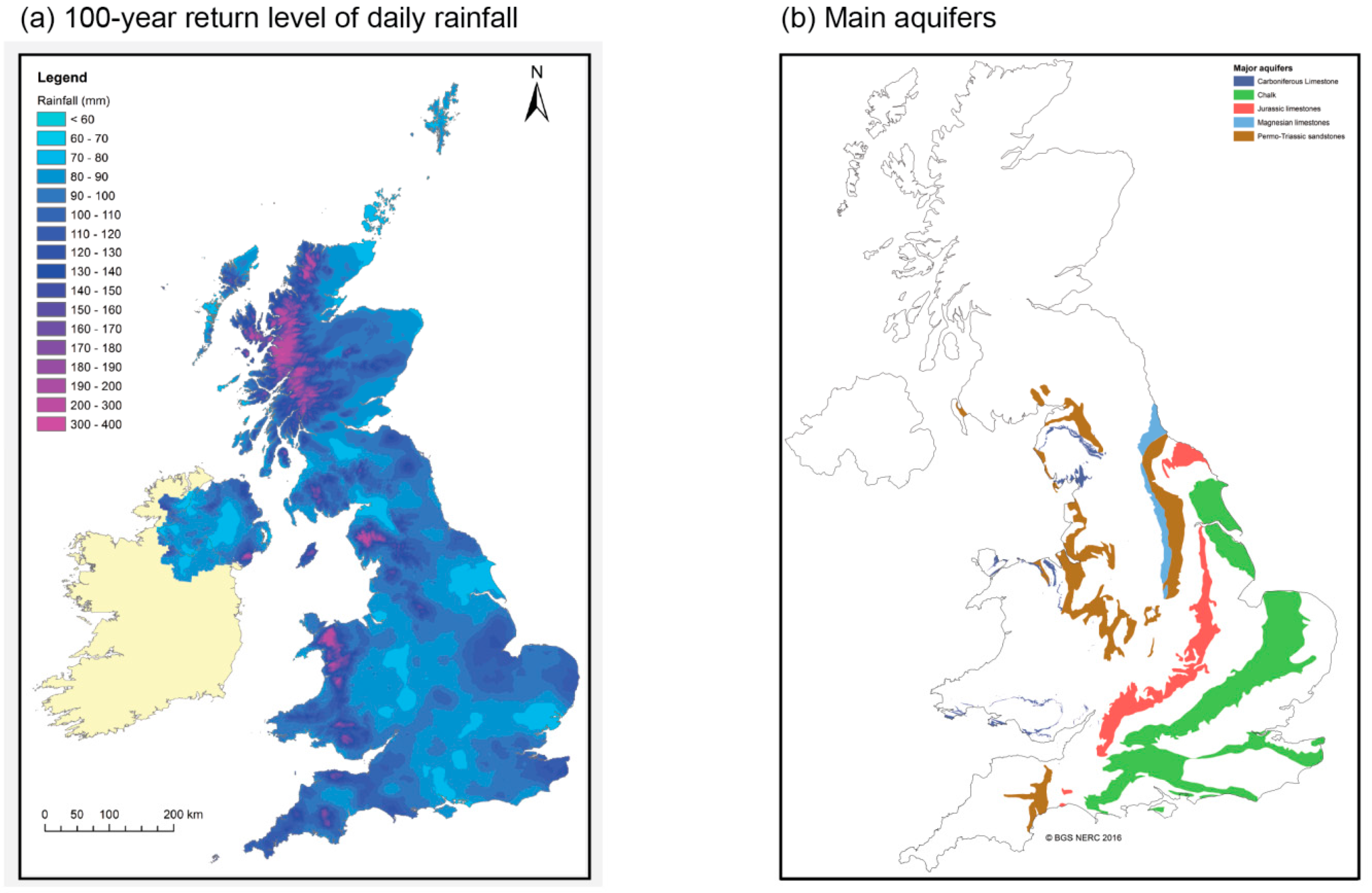
2.1. The Future Flow Database

The analysis is based on the Future Flows database which was developed to provide a consistent set of transient daily river flow and monthly groundwater level projections across England, Wales and Scotland (281 stations). Future Flows Hydrology is derived from Future Flows Climate [33], an 11-member ensemble of transient climate projections for Great Britain (bias-corrected and downscaled on a 1-km grid) based on HadRM3-PPE-UK, developed as part of the derivation of the UKCP09 scenarios [34]. HadRM3-PPE-UK was designed to represent parameter uncertainty in climate change projections through a parameter variant experiment and was run under the SRES A1B emissions scenario (see [19] for details of the climate model perturbations). Future Flows Hydrology contains an 11-member ensemble of transient projections from January 1951 to December 2098, each associated with a single realisation from a different variant of HadRM3. Note that [19] stipulates that daily time series from particular HadRM3-PPE member should be interpreted as plausible realisations, but cannot be associated with level of probabilities. As the 11-member HadRM3-PPE-UK was finalised after elimination of unrealistic simulations by the original 17-member ensemble [19,35], each ensemble member was considered in this study as plausible and all equally probable.

2.2. Block Maxima and Peak over Threshold Methods

The hydrological dataset is analysed using EV theory [21], specifically two different EV models were used in order to investigate the uncertainty associated with model structure (i.e., model choice) and model parameters (i.e., fitting/sampling error): (i) the GEV for block maxima (Equation (1), here a block was considered as a year, i.e., annual maxima values were used); and (ii) the GP for threshold exceedances (Equation (2)).

The EV theory considers (X₁, X₂, …, X_n) a sequence of independent random variables and M_n = max{X₁, X₂, …, X_n} a sequence of block maxima [21]. If there are a_n > 0 and b_n, such that the probability $\mathrm{Pr}\left\{\frac{M_n-b_n}{a_n}\le z\right\}\to G(z)$, then:

(i)

G(z) belongs to the GEV family distribution:

$$G(z)=\exp \left\{-{\left[1+\xi \left(\frac{z-\mu }{\sigma }\right)\right]}_{+}^{-1/\xi }\right\}$$

(1)

with μ the location parameter, σ > 0 the scale parameter, and ξ (≠0) the shape parameter.

(ii)

For large enough u, the distribution function of y = X − u conditional on X > u, is approximately the GP distribution:

$$H(y)=1-{\left(1+\xi \frac{y}{\sigma }\right)}_{+}^{-1/\xi }$$

(2)

Both models were fit with the R package “extRemes” [36] using the Maximum Likelihood Estimation (MLE) method and profile likelihood was used to obtain the 95% confidence intervals (CI) to capture the uncertainty associated with the EV model parameters. MLE is one of the most commonly used for parameter estimation for EV models [37] and is valid for samples of size n > 25 [38]. The profile likelihood intervals were calculated with the R function ci.fevd (package extRemes). This function was implemented with a range of [0.5 × estimate, 1.5 × estimate], which was defined using a trial-and-error approach to be large enough to cover the 95% CI.

2.3. Automated Computing

To automatically select the best threshold for the POT of each series, the ATSM approach [30] was applied on the declustered runoff series to ensure data independence. Declustering runoff series consists in selecting “clusters”, or groups of dependent runoff values, and extracting the maximum value of each cluster. That step was performed based on the “Runs declustering” method [21]: the extreme runoff separated by fewer than r non-extremes (r = 7 in this study) were considered the same cluster. Note that the r value was chosen after a sensitivity analysis on the Extremal Index to ensure all the POT series were independent. This resulted in an Extremal Index of above 0.997 for all stations, for all ensemble members over both time periods.

The ATSM runs as follow:

• Identify a series of n suitable thresholds, u₁ < u₂ < … < u_n, equally spaced, between the median and the 98% quantile of the data series. For j = 1, …, n, fit a GP model and estimate the likelihood estimator of the scale (σ_uj) and shape (ξ_uj) parameters for the declustered data above the threshold u_j.
• Test the sequence (τ(u_j) − τ(u_j−1))_{j=2, …, n} for j = 1 against the Pearson’s Chi-square Test, with the test variable τ(u_j) = σ_uj − ξ_uj × u_j. For any u < u_j−1 < u_j, the difference τ(u_j) − τ(u_{j − 1}) is approximately normally distributed with mean 0. If the null hypothesis of normality is rejected then u₁ is not a suitable threshold.
• Repeat Step 2 for j = 2, …, n if u₁ is not suitable, until finding and extracting the first threshold u_j for which the difference sequence fulfils the normality condition.

Then, using the defined series (AM or POT), the GEV and GP models are fitted to the daily flow database across Great Britain for the 11-member ensemble on the baseline (1961–1990) and for the 2080s (2069–2098). Once fitted, they are used to assess the 1:100 yrF.

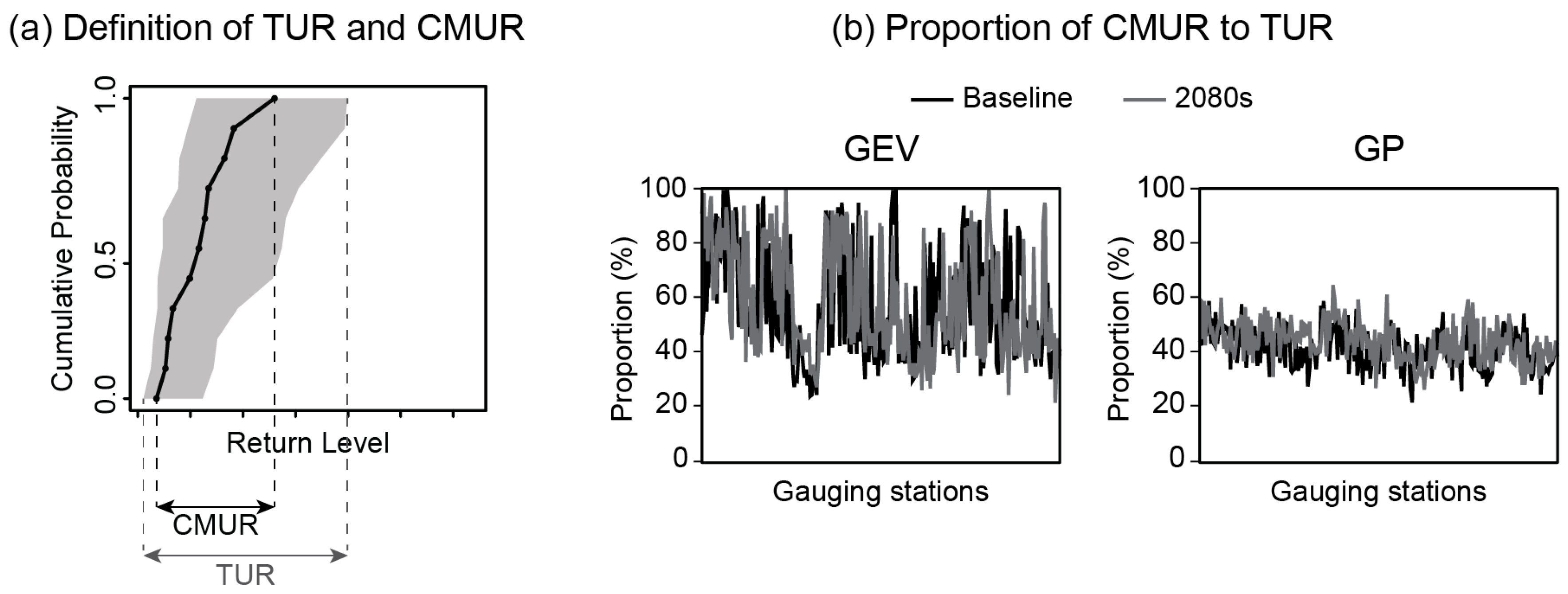
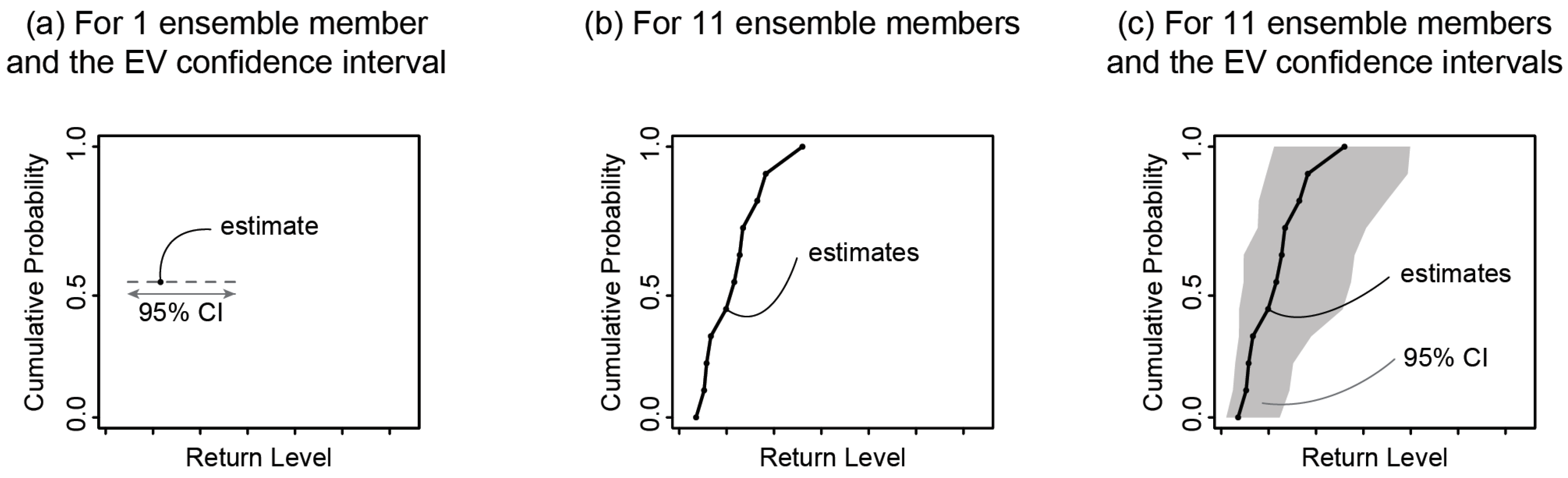
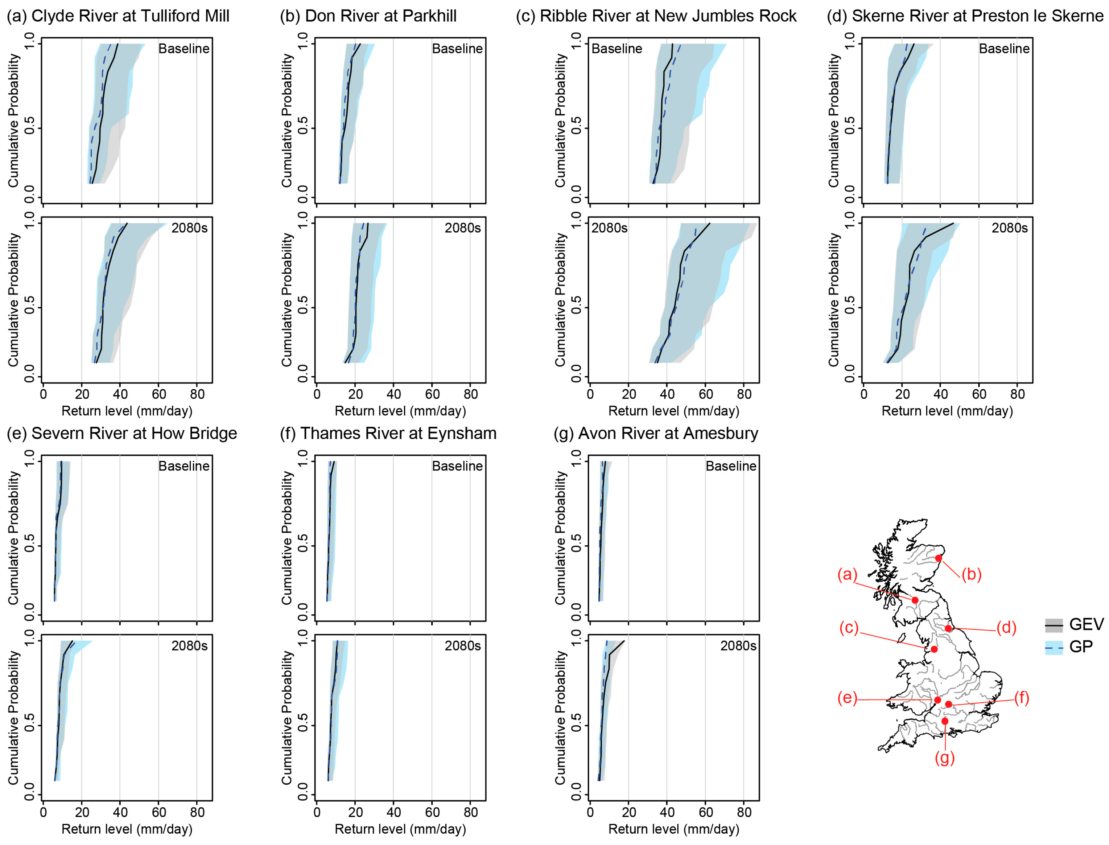
2.4. Assessment of Uncertainties Associated with the Return Level Estimate

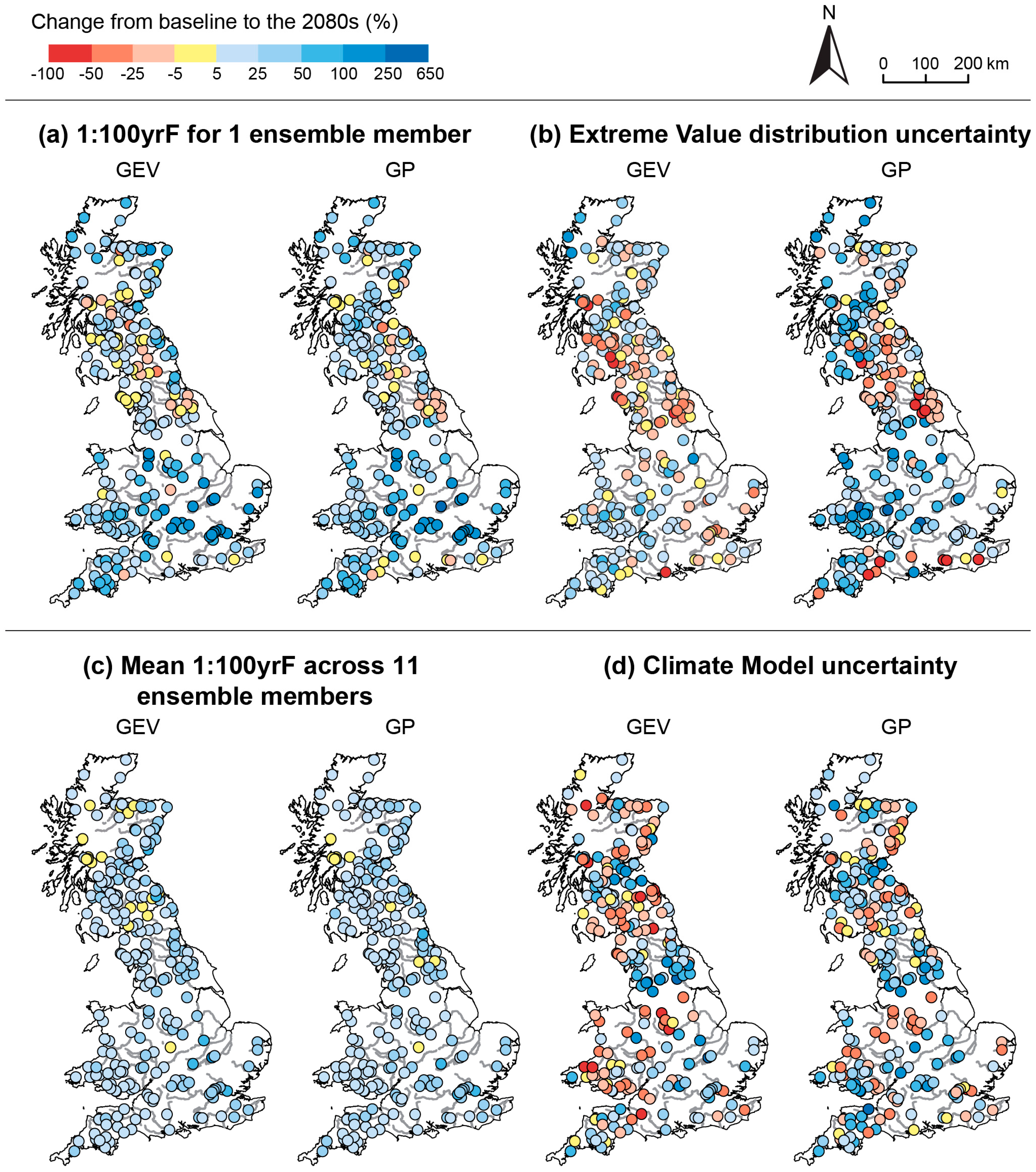
The analysis is carried out in three main steps:

The first step investigates the uncertainty related to the EV models (GEV and GP) parameters, and by comparison the model structure. This is undertaken for each station (281), for both time periods. For each station, and for only one ensemble member, the 1:100 yrF and its 95% confidence interval are assessed using the profile likelihood method (see Figure 2a). Ensemble member afgcx was chosen for this, as this is the original RCM HadRM3-PPE member. The 10 other ensemble members represent slightly different model physics. To ensure a normative comparison across Great Britain, and thus to remove the bias related to the underlying climate, a relative coefficient of uncertainty is computed (Equation (3)):

$$R{C}_U=\frac{C{I}_{up}-C{I}_{low}}{E}$$

(3)

with E the runoff estimate, CI_up the upper 95% confidence limit, and CI_low the lower 95% confidence limit. This coefficient is dimensionless and allows the comparison of CI ranges for locations with different 1:100 yrF estimates for both the GEV and GP models. Note that this is a relative measure of uncertainty since larger peak flows tend to have larger the confidence intervals associated which leads to higher absolute uncertainty. Thus the CI captures the uncertainty in model fitting, whilst combining the uncertainty from both methods allows the uncertainty in model structure to be captured.

The second step investigates the uncertainty related to the climate model (CM) parameters. Return levels are computed for the 11 ensemble members, resulting in an empirical Cumulative Distribution Function (CDF, see Figure 2b) for the baseline and the 2080s assuming an equal probability of each of the 11 ensemble members. The relative standard deviation across the 11 ensemble members is calculated for each station (Equation (4)).

$$RSD=\frac{s}{m}$$

(4)

with s the sample standard deviation and m the sample mean of the distribution. The relative standard deviation is a standardized measure of dispersion of a probability distribution. It is a dimensionless number, expressed in percentage, which allows the comparison between data with different means and dispersions.

The third step graphically represents the combined uncertainties associated with assessing return level estimates with each EV model for the 11 ensemble members. This is presented through a smoothed empirical CDF of the estimates and their associated 95% confidence intervals (see Figure 2c).

Using the ATSM approach, some stations (less than 10%) had less than one POT per year on average for an independent series, thus these stations were removed from the analysis.

3. Results

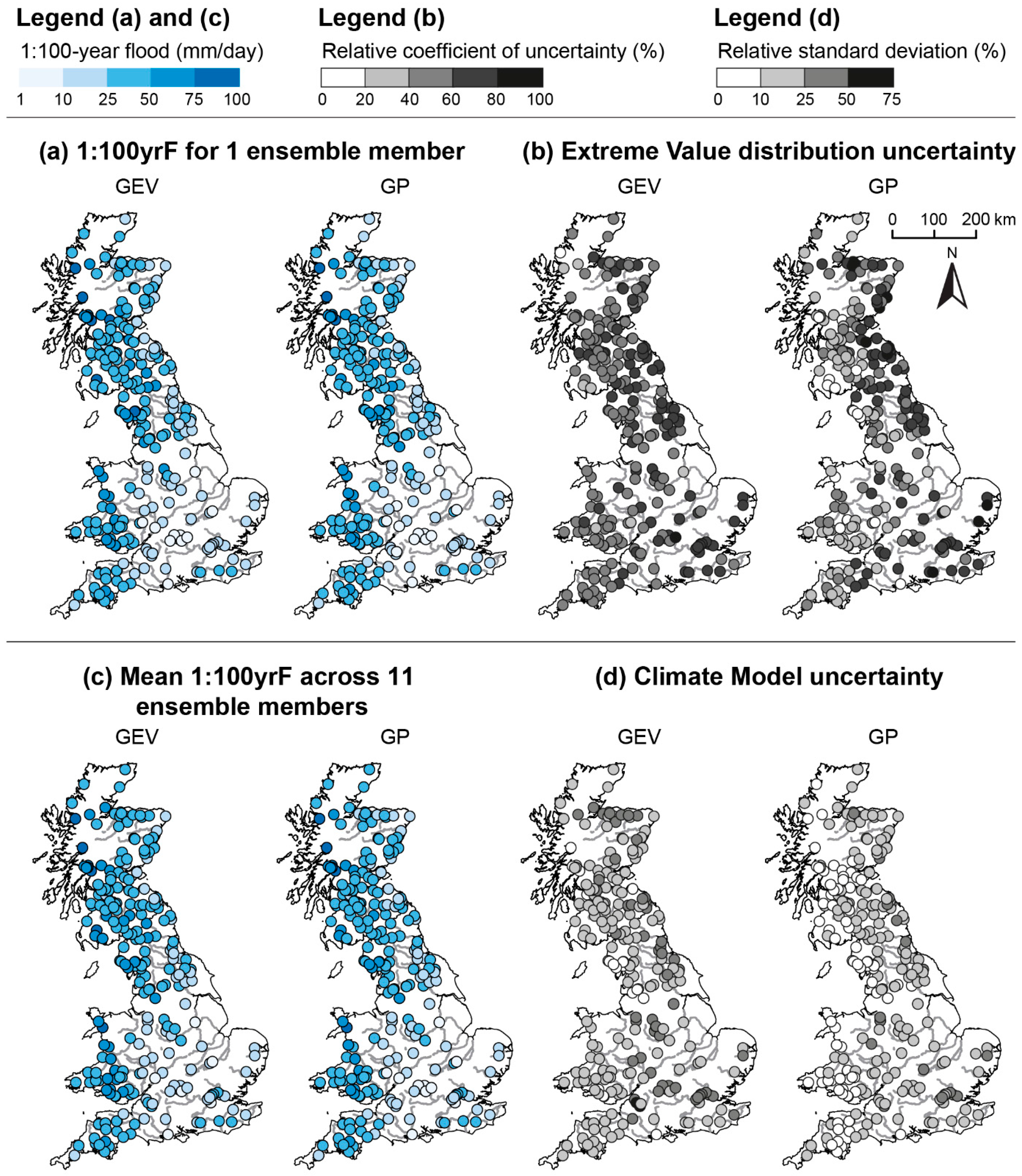
3.1. Uncertainties on the Baseline

Figure 3 shows the 1:100 yrF calculated for the baseline across Great Britain with the GEV and the GP models for one ensemble member (Step 1, Figure 2a) and the associated uncertainty (Step 1, RC_U: Equation (3), the relative 95% CI range for 1 ensemble member); and the mean value across the 11 ensemble members (Step 2, Figure 2b) and the associated uncertainty (Step 2, RSD: Equation (4), the relative standard deviation across 11 ensemble members).

Figure 3a shows that the GEV model suggests slightly higher 1:100 yrF estimates than the GP model for 73% of stations (e.g., river Clyde at Sills of Clyde: 33 mm with GEV and 32 mm with GP). Figure 3b shows that the EV uncertainty is lower with GP (60% of stations), especially on the west coast (e.g., river Teifi at Llanfair: RC_U of 73% with GEV and 55% with GP), but for some sites can be higher, particularly on the east coast (e.g., river Waveney at Needham Mill: RC_U of 79% with GEV and 86% with GP). Figure 3c shows that the mean 1:100 yrF tends to be slightly higher with the GEV (89% of stations, e.g., river Alness at Alness: 51 mm with GEV and 43 mm with GP) and Figure 3d shows that the CM uncertainty is lower with the GP (82% of stations), especially along the west coast (e.g., river Girvan at Robstone: 15% with GEV and 8% with GP).

3.2. Change in Flood Peak by the 2080s

Figure 4 shows the percentage change in 1:100 yrF and the associated uncertainties arising from model parameters (EV and CM) from the baseline to the 2080s across Great Britain for the GEV and the GP models. Change in 1:100 yrF for one ensemble member and change in EV uncertainty are shown in Figure 4a,b respectively. Changes in the mean value across the 11 ensemble members and in CM uncertainty are shown in Figure 4c,d respectively. Increasing trends are shown in blue shades while decreasing trends are shown in red shades and no significant changes are shown in light yellow.

Figure 4a shows that for one ensemble member and both the GEV and GP models, the 1:100 yrF decreases from the baseline to the 2080s in some stations in Scotland and the north of England (e.g., −38% for the South Tyne at Haydon Bridge) and increases for the rest of Great Britain (87% of stations), with the highest increase in southeast of England (e.g., +293% for the Belchamp Brook at Bardfield Bridge). This change is related to the predicted change to climate in this region and how the geographical and landscape controls translate these to changes in runoff. Figure 4b shows that for the GEV model, the EV model uncertainty decreases in west of Scotland (e.g., −58% for Falloch River at Glen Falloch) and north and southeast of England (e.g., −31% for the Belchamp Brook at Bardfield Bridge) and increases in the rest of Great Britain (63% of stations, up to 255% for the Browney River at Burnhall). This trend is more acute for the GP model (73% of stations), with the highest increase in south of England (e.g., +640% for the Kennet river at Newbury).

Figure 4c shows that for the 11 ensemble members and both the GEV and GP models, the mean 1:100 yrF would increase from the baseline to the 2080s across Great Britain (in 97% and 98% of stations for GEV and GP respectively), apart from isolated stations in Scotland and the south of England. The largest 1:100 yrF increases remain in southeast of England (e.g., +101% for the Kym river at Meagre Farm). Figure 4d shows that for the GEV model, the CM uncertainty mainly increases (70% of stations), especially in Scotland (e.g., +169% for the Avon river at Polmonthill) and north of England (e.g., +289% for the Wharfe River at Flint Mill Weir), and decreases in the south of Scotland, Wales, and central England (e.g., −51% for the Dove River at Hollinsclough). For the GP model, the trend follows the same pattern (increase at 66% of stations), with the highest increase in south of England (+487% for the Silk Stream at Colindeep Lane) and highest decrease in central England (−55% for the Manifold River at Ilam).

3.3. Combined Uncertainties

Figure 5 shows the estimated 1:100 yrF for the 11 ensemble members calculated with the GEV and the GP models and the associated 95% CI which captures EV model parameter uncertainty (Step 3, see Figure 2c) for the baseline and the 2080s. This figure shows the total uncertainty in return level estimate for each of these gauging stations, whilst also clearly showing the uncertainty attributable to each source (i.e., CM parameters, EV model parameters and EV model structure). Seven gauging stations representative of their region were chosen across Great Britain (see bottom left of the figure for station location): the Clyde and the Don rivers in west and east of Scotland, respectively (Figure 5a,b); the Ribble and Skerne rivers in west and east of north England, respectively (Figure 5c,d); the Severn and Thames rivers in west of Wales and southeast of England, respectively (Figure 5e,f); and the Avon river in south of England (Figure 5g).

The GEV and the GP models compute similar 1:100 yrF for all stations. For both EV models, the highest 1:100 yrF are found on the western stations (the Clyde and the Ribble), while the southern stations present the lowest 1:100 yrF (the Severn, the Thames and the Avon). For all stations, there is an increase in 1:100 yrF from baseline to the 2080s. The CM uncertainty increases from baseline to the 2080s especially for the Ribble, the Skerne, and the Avon. Similarly, the EVD uncertainty increases notably from baseline to the 2080s for these three stations.

Finally we consider the uncertainty attributable to the EV model structure by combining the GEV and GP uncertainty envelopes on the baseline and the 2080s. From this we can quantify the range of CM parameter uncertainty that contributes to the total uncertainty range.

Table 1. For each selected gauging station, on the baseline and the 2080s: combined GEV and GP model uncertainties related to the climate model (CCMU) and the total combined cascaded uncertainty (TCCU).

River	CCMU (mm) Baseline	CCMU (mm) 2080s	TCCU (mm) Baseline	TCCU (mm) 2080s
Clyde	13.66	16.37	30.16	40.13
Don	10.81	12.08	19.62	23.39
Ribble	14.39	28.19	39.82	56.13
Skerne	14.07	35.41	25.97	42.70
Severn	3.84	10.08	8.63	18.11
Thames	4.11	4.96	5.54	10.22
Avon	3.39	13.64	7.41	14.15

presents, for each station in Figure 5, the combined uncertainties from both models (GEV and GP) related to the climate model (CCMU), i.e., the range in estimate values (see Equation (5)), and the total combined cascaded uncertainty (TCCU) (see Equation (6)).

$$CCMU=\max \left\{\max (E_{GEV}),\max (E_{GP})\right\}-\min \left\{\min (E_{GEV}),\min (E_{GP})\right\}$$

(5)

with max(E_GEV) and max(E_GP) the maximum estimate computed by the GEV and the GP, respectively, and min(E_GEV) and min(E_GP) the minimum estimate computed by the GEV and the GP, respectively.

$$TCCU=\max \left\{\max (C{I}_{up,GEV}),\max (C{I}_{up,GP})\right\}-\min \left\{\min (C{I}_{low,GEV}),\min (C{I}_{low,GP})\right\}$$

(6)

with max(CI_up,GEV) and max(CI_up,GP) the maximum upper 95% confidence limit computed by the GEV and the GP, respectively, and min(CI_low,GEV) and min(CI_low,GP) the minimum lower 95% confidence limit computed by the GEV and the GP, respectively.

The highest uncertainties are found in the northern stations, particularly on the Ribble River, where the 1:100 yrF values are higher. CCMU increases from baseline to the 2080s for all stations, especially on the Ribble, the Severn, and the Avon where it doubles. TCCU increases for all the stations; it doubles for all of them except for the Skerne and the Avon rivers where it stays stable.

4. Discussion

4.1. Main Results

4.1.1. National Picture

Across Great Britain the GEV and the GP models generally suggest similar magnitude and spatially contrasted 1:100 yrF estimates. The highest 1:100 yrF are observed on the west coast, with the lowest climate model and EV model uncertainties. In contrast, the lowest 1:100 yrF are found in south and southeast of England, with the highest uncertainties. By the 2080s, the results show a general increase to 1:100 yrF estimates across Great Britain, with the highest in south England. The CM and EVD uncertainties mainly increase in central Scotland, north England, south England and Wales, and decrease in central England. The increase in uncertainty between the baseline and the future is slightly higher for the GP than the GEV model across the country. The increased trend of EV uncertainty associated with the GP model is correlated to the decreasing number of POT from baseline to the 2080s for 86% of the stations (on average 1 POT per year), resulting in an increase in uncertainty of the GP model fitting. Figure 3 is explained by the hydro-climatic context of Great Britain, whereby the gradient in 1:100 yrF follows the observed gradient of 1:100-year rainfall (see Figure 1a). The hydrological response of west coast catchments follows the rainfall signal. Moreover, the higher uncertainty found in southeast England may be related to the significant groundwater signal of these catchments (see Figure 1b).

Regarding uncertainties on the baseline, Figure 3b shows that the 95% confidence interval can be as large as the 1:100 yrF estimate, resulting in relative coefficient of uncertainty values of up to 100% particularly on the west and the south coast of Great Britain. The estimation of the 1:100 yrF on the baseline can thus be associated to a high uncertainty related to the EV model parameter for these stations. Moreover, the 1:100 yrF estimate in the 2080s stays within the baseline Total Uncertainty Range (TUR, see Figure 6a) for the vast majority of the stations (99% and 100% with the GEV and GP, respectively). This is illustrated in Figure 5. However, it is important to note that the future estimate plus its associated uncertainty bounds exceeds those on the baseline (estimate plus uncertainty): the upper 95% confidence limit is higher in the 2080s than on the baseline for 92% and 88% of the stations with the GEV and the GP, respectively, and the 1:100 yrF estimate consistently increases from the baseline to the 2080s across Great Britain (see Figure 4c). Hence, when the total uncertainty in the future estimate is captured, this exceeds all baseline estimates. Thus, the use of Climate Model simulations in the future allows capturing the change in uncertainty for design flood estimates.

4.1.2. Cascading Uncertainties

Results show that, based on the same hydro-climatic simulations, the GEV and GP models provide different levels of uncertainty when estimating the 1:100 yrF. Figure 6b investigates for all the gauging stations across Great Britain the relative range of uncertainty arising from the CM parameters (CMUR, see Figure 6a), compared to the total range of uncertainty obtained after cascading the uncertainty related to the CM parameters into the EV models (TUR, see Figure 6a). Since the CMU is cascaded into the EV model parameter uncertainty, the CMU and EVDU are not additive. However, by understanding the proportion of TUR which is attributable to CMU, we can understand and quantify the extra uncertainty which is attributable to the EV model parameter for the GEV and GP results separately, and by combination of the EV model structure. Hence, we can highlight the level of uncertainty which may be overlooked if EV uncertainty is not considered within the process.

With the GEV, the proportion of uncertainty arising from the CM is similar on the baseline and the 2080s (58% and 59% for the baseline and the 2080s, respectively), and varies greatly amongst the gauging stations (from 24% to 99%). The GEV model is more sensitive to the input data and therefore if the CMU is taken into account only, around 40% of the total uncertainty in 1:100 yrF estimation is overlooked. In contrast, the proportion of the total uncertainty attributed to the CM for the GP model is lower (42% on the baseline and 44% on the 2080s). Hence a larger amount of information on uncertainty (almost 60%) is missing when capturing CM uncertainty alone. Nationally, the uncertainties are more constrained for GP than for GEV. This analysis suggests that when using Extreme Value models it is critical to capture the parameter uncertainty. Considering CMU alone overlooks the extra uncertainty which arises from the extreme value model.

Thus far, the results have analysed the individual behaviour of both the GEV and GP when cascading the CMU into the EV models for the 1:100 yrF assessment. At the national scale, we saw that the RC_U (that quantifies the EV uncertainty calculated for ensemble member afgcx) increased from baseline to the 2080s for 63% and 73% of stations (GEV and the GP respectively). Similarly, the RSD (that quantifies the CMU across the 11 ensemble-members) increased from the baseline to the 2080s for 56% and 66% of stations (GEV and the GP respectively). When both models are merged, i.e., when the uncertainty related to the extreme value model structure is also taken into account, as illustrated in Figure 5, the total uncertainty range increases for each station, on both the baseline and the 2080s. It is clear from the results that the estimate and the uncertainty associated with it are strongly determined by individual constraints in each catchment. In some catchments CM uncertainties dominate (e.g., the Thames and the Don Rivers), while in others EV model uncertainty is critical (e.g., Skerne and Severn Rivers). Moreover, from the baseline to the 2080s, there is an increase in RC_U for 64% of stations and in RSD for 59% of stations. This suggests that for the majority of catchments the total cascaded uncertainty increases from the baseline to the future, however in a significant number of catchments across the UK it remains stable or decreases.

4.1.3. GEV vs. GP and Automated Procedure

One of the challenges of this large-scale analysis was automatically calculating 1:100 yrF using the GP model. Various automated methods are presented in the literature [39]. Given the large amount of data analysed in this study, we chose a robust and computer-efficient method developed by [30] and applied it on declustered data series to ensure peak data independency.

The main difference of this method from the one generally used by UK Environment Agencies is that they manually update the chosen threshold to result in five peaks per year and ensure independency by detailed inspection [29]. In this study, after declustering each 30-year series ensuring peak runoff independence, the ATSM approach selected one threshold value for each series, resulting in between 1 and 13 POTs per year at each station, which raises the question of validity of the GP model and its relative merits compared to the GEV model. However for the purposes of this study, and by using both the GEV and GP methods we have understood the difference in estimate across the UK, and captured the uncertainty associated with model parameters.

4.2. Limits

Some limits of this study are related to the use of the Future Flow database. As reported by [20], three models are used to simulate river flow (CERF [40], PDM [41], and CLASSIC [42]) with the emphasis of calibration on different parts of the flow regime. For CERF the emphasis is on the representation of the water balance and low flows, while for PDM and CLASSIC the emphasis is on the upper part of the flow regime and peak flows. For the gauging stations calibrated with the CERF model, the estimated 1:100 yrF might thus be under-estimated.

The ATSM failed for less than 10% of the gauging stations for which the automated selected threshold induced on average less than 1 POT per year (not shown in Figure 3 and Figure 4). The affected stations are located in southeast of England and correspond to rivers linked to the chalk aquifers (see Figure 1b). The flow regime at these stations is mainly controlled by the baseflow provided by underground reservoirs. For these catchments, the selection of independent peak flows using the declustering technique resulted in most peaks being removed due to inter-dependency. The resulting GP model which was fitted contained uncertainties due to the lack of data available to estimate its parameters, and thus were removed from this analysis.

Finally, this study investigates the uncertainty related to one climate model only (HadRM3), under one forcing scenario (emission scenario). Using a wide range of General Circulation Models (GCMs) outputs is generally recommended to estimate a set of possible futures in impact studies, as well as the probability of occurrence of these future scenarios [17]. Additional sources of uncertainty such as input data forcing the climate model (i.e., the chosen emission scenario) [43] could also be taken into account, and would probably lead to a larger range of possible peak flows. Probabilistic approaches allow the uncertainty of climate models outputs to be characterized and sensitivity and performance of impact models evaluated based on these uncertainties. However, as reported by [44], these uncertainties can range widely, related to divergent GCMs outputs with large biases in simulation, especially precipitation, resulting in little concluding information for impact studies.

5. Conclusions

The aim of this study was to assess the change to extreme runoff estimates across Great Britain in the future as a result of climate change and quantify the uncertainties related to climate model parameters as well as the extra uncertainty arising from choosing and fitting Extreme Value models.

The main results of the study suggest that the two investigated EVD (GEV and GP) provide similar estimates of future extreme events. The west coast of Great Britain is likely to experience the highest 1:100 yrF but with low associated uncertainty. The south and southeast of England are likely to experience the lowest 1:100 yrF but with the highest uncertainty. From the baseline to the 2080s, there is an increase in 1:100 yrF and an increase in the associated uncertainty in the estimate, particularly in southeast of England. The uncertainty related to the climate model and the EV model parameters can be similar, which shows the importance of accounting for both of them in future studies. However, for some catchments CM uncertainties dominate, while for others EV model uncertainties are at least as significant. This is an important finding as CM uncertainties are often considered, if not quantified, while EV model uncertainty is widely overlooked.

Moreover, the uncertainty induced on the baseline, particularly from the EV model parameters, can be significantly large. Indeed the results show that the 1:100 yrF estimate in the 2080s stays within the baseline uncertainty bounds. However, the uncertainty associated with this future estimate exceeds the uncertainty range on the baseline across the UK. This suggests that current knowledge of uncertainties arising from the standard modelling chain are likely to be significant for future design flood assessment and as a result we suggest that this supports the need to incorporate CM simulations in future design flood estimates. Probabilistic approaches need to be developed [44] to cascade these uncertainties into flood risk mapping in order to assess the influence these uncertainties have on future flood exposure.

This paper has taken a national approach to analyse the impact of climate change to future 1:100 yrF, incorporating the uncertainty in climate model and EV model parameters as well as EV model structure. Such a national approach is critical for understanding potential climate change impacts. Based on the findings this paper suggests that uncertainties attributable to both climate and extreme value models should be explicitly considered in future assessments of extreme events. Ultimately these uncertainties should be cascaded through to the estimate of flood hazard and exposure to understand the potential future change to inundation extent in the future. This raises the issue of research communication to stakeholders and how statistical methods and results can be transferred for use by water managers and decision makers. Nowadays deterministic approaches are used for Flood Risk Assessment [22] and there is an urgent need to move towards probabilistic frameworks to better anticipate Climate Change impact by understanding the associated uncertainties and quantify ranges of possible futures. Probabilistic approaches can be developed [45] to cascade these uncertainties into flood risk mapping and assess the resulting likely design flood in both past and future time periods. This would allow a better understanding of future possible flood risk by constraining the uncertainties with the catchment physical processes and characteristics. Further research should also investigate the regional patterns of extreme peak flow events, and the uncertainties related to climate models and extreme value models, in order to perform a regionalization analysis to apply these trends on ungauged catchments. This would provide a useful tool to stakeholders for application to practical case studies to account for climate change impact.

References

1. Jonkman, S.; Vrijling, J. Loss of life due to floods. J. Flood Risk Manag. 2008, 1, 43–56. [Google Scholar] [CrossRef]
2. Guha-Sapir, D.; Below, R.; Hoyois, P. Natural Disasters Reported. EM-DAT: International Disaster Database; Université Catholique de Louvain: Brussels, Belgium, 2015. [Google Scholar]
3. Kantamaneni, K.; Phillips, M. Transformation of climate: Will floods and coastal erosion crumble the UK economy? Int. J. Clim. Chang. Impacts Responses 2016, 8, 45–59. [Google Scholar]
4. Alfieri, L.; Feyen, L.; di Baldassarre, G. Increasing flood risk under climate change: A pan-European assessment of the benefits of four adaptation strategies. Clim. Chang. 2016, 136, 507–521. [Google Scholar] [CrossRef] [Green Version]
5. Wagenaar, D.J.; de Bruijn, K.M.; Bouwer, L.M.; de Moel, H. Uncertainty in flood damage estimates and its potential effect on investment decisions. Nat. Hazards Earth Syst. Sci. 2016, 16, 1–14. [Google Scholar] [CrossRef]
6. UK Parliament. Current Parliamentary Material Available on Flooding. Available online: http://www.parliament.uk/topics/Flooding.htm (accessed on 16 August 2013).
7. Stewart, L.; Vesuviano, G.; Morris, D.; Prosdocimi, I. The new FEH rainfall depth-duration-frequency model: Results, comparisons and implications. In Proceedings of the 12th British Hydrological Society National Symposium, Birmingham, UK, 2–4 September 2014; Available online: http://nora.nerc.ac.uk/510563/ (accessed on 23 March 2016).
8. Wilby, R.L.; Beven, K.J.; Reynard, N.S. Climate change and fluvial flood risk in the UK: More of the same? Hydrol. Process. 2008, 22, 2511–2523. [Google Scholar] [CrossRef]
9. Faulkner, D. Rainfall Frequency Estimation. In Flood Estimation Handbook; Institute of Hydrology: Wallingford, UK, 1999; Volume 2, 110p. [Google Scholar]
10. Arnell, N.W.; Gosling, S.N. The impacts of climate change on river flood risk at the global scale. Clim. Chang. 2016, 134, 387–401. [Google Scholar] [CrossRef]
11. Di Baldassarre, G.; Schumann, G.; Bates, P.; Freer, J.; Beven, K. Flood-plain mapping: A critical discussion of deterministic and probabilistic approaches. Hydrol. Sci. J. 2010, 55, 364–376. [Google Scholar] [CrossRef]
12. Beevers, L.; Douven, W.; Lazuardi, H.; Verheij, H. Cumulative impacts of road developments in floodplains. Transp. Res. D 2012, 17, 398–404. [Google Scholar] [CrossRef]
13. Balica, S.; Beevers, L.; Popescu, I.; Wright, N. Parametric and physically based modelling techniques for flod risk and vulnerability assessment: A comparison. Environ. Model. Softw. 2013, 41, 81–92. [Google Scholar] [CrossRef]
14. Beven, K.; Hall, J. (Eds.) Applied Uncertainty Analysis for Flood Risk Management; Imperial College Press: London, UK, 2014.
15. Von Christierson, B.; Wade, S.; Counsell, C.; Arnell, N.; Charlton, M.; Prudhomme, C.; Hannaford, J.; Lawson, R.; Tattersall, C.; Fenn, C.; et al. Climate Change Approaches in Water Resources Planning—Overview of New Methods; Report SC090017/R3; Environment Agency: London, UK, 2013.
16. Prudhomme, C.; Jakoba, D.; Svensson, C. Uncertainty and climate change impact on the flood regime of small UK catchments. J. Hydrol. 2003, 277, 1–23. [Google Scholar] [CrossRef]
17. Wilby, R.L. Evaluating climate model outputs for hydrological applications. Hydrol. Sci. J. 2010, 55, 1090–1093. [Google Scholar] [CrossRef]
18. Augustin, N.; Beevers, L.; Sloan, W. Predicting river flows for future climates using an autoregressive multinomial logit model. Water Resour. Res. 2008, 44. [Google Scholar] [CrossRef]
19. Murphy, J.M.; Sexton, D.M.H.; Jenkins, G.J.; Boorman, P.M.; Booth, B.B.B.; Brown, C.C.; Clark, R.T.; Collins, M.; Harris, G.R.; Kendon, E.J.; et al. UK Climate Projections Science Report: Climate Change Projections; Met Office Hadley Centre: Exeter, UK, 2009. [Google Scholar]
20. Prudhomme, C.; Haxton, T.; Crooks, S.; Jackson, C.; Barkwith, A.; Williamson, J.; Kelvin, J.; Mackay, J.; Wang, L.; Young, A.; et al. Future Flows Hydrology: An ensemble of daily river flow and monthly groundwater levels for use for climate change impact assessment across Great Britain. Earth Syst. Sci. Data 2013, 5, 101–107. [Google Scholar] [CrossRef] [Green Version]
21. Coles, S. An Introduction to Statistical Modelling of Extreme Values; Springer: London, UK, 2001. [Google Scholar]
22. Centre for Ecology & Hydrology. Flood Estimation Handbook; Centre for Ecology & Hydrology: Wallingford, UK, 1999; Volumes 1–5. [Google Scholar]
23. Bocchiola, D.; De Michele, C.; Rosso, R. Review of recent advances in index flood estimation. Hydrol. Earth Syst. Sci. 2003, 7, 283–296. [Google Scholar] [CrossRef]
24. Svensson, C.; Jones, D. Review of rainfall frequency estimation methods. J. Flood Risk Manag. 2010, 3, 296–313. [Google Scholar] [CrossRef] [Green Version]
25. Prosdocimi, I.; Kjeldsen, T.; Miller, J. Detection and attribution of urbanization effect on flood extremes using nonstationary flood-frequency models. Water Resour. Res. 2015, 51, 4244–4262. [Google Scholar] [CrossRef] [PubMed] [Green Version]
26. Esteves, L.S. Consequences to flood management of using different probability distributions to estimate extreme rainfall. J. Environ. Manag. 2013, 115, 98–105. [Google Scholar] [CrossRef] [PubMed]
27. Madsen, H.; Rasmussen, P.; Rosbjerg, D. Comparison of annual maximum series and partial duration series methods for modeling extreme hydrologic events, 1, At-site modeling. Water Resour. Res. 1997, 33, 747–757. [Google Scholar] [CrossRef]
28. Ferreira, A.; de Haan, L. On the block maxima method in extreme value theory: PWM estimator. Ann. Stat. 2015, 43, 276–298. [Google Scholar] [CrossRef]
29. Bayliss, A.C.; Jones, R.C. Peaks-over-Threshold Flood Database: Summary Statistics and Seasonality; IH Report No. 121; Institute of Hydrology: Wallingford, UK, 1993; 68p. [Google Scholar]
30. Thompson, P.; Cai, Y.; Reeve, D.; Stander, J. Automated threshold selection methods for extreme wave analysis. Coast. Eng. 2009, 56, 1013–1021. [Google Scholar] [CrossRef]
31. Fukutome, S.; Liniger, M.A.; Süveges, M. Automatic threshold and run parameter selection: A climatology for extreme hourly precipitation in Switzerland. Theor. Appl. Climatol. 2013, 120, 403–416. [Google Scholar] [CrossRef]
32. Süveges, M.; Davison, A.C. Model misspecification in peaks over threshold analysis. Ann. Appl. Stat. 2010, 4, 203–221. [Google Scholar] [CrossRef]
33. Prudhomme, C.; Dadson, S.; Morris, D.; Williamson, J.; Goodsell, G.; Crooks, S.; Boelee, L.; Davies, H.; Buys, G.; Lafon, T.; et al. Future Flows Climate: An ensemble of 1-km climate change projections for hydrological application in Great Britain. Earth Syst. Sci. Data 2012, 4, 143–148. [Google Scholar] [CrossRef] [Green Version]
34. Murphy, J.M.; Booth, B.B.B.; Collins, M.; Harris, G.R.; Sexton, D.M.H.; Webb, M.J. A methodology for probabilistic predictions of regional climate change from perturbed physics ensembles. Philos. Trans. R Soc. A 2007, 365, 1993–2028. [Google Scholar] [CrossRef] [PubMed]
35. Brown, I.; Poggio, L.; Gimona, A.; Castellazzi, M. Climate change, drought risk and land capability for agriculture: Implications for land use in Scotland. Reg. Environ. Chang. 2011, 11, 503–518. [Google Scholar] [CrossRef]
36. Gilleland, E.; Katz, R.W. New software to analyze how extremes change over time. Eos 2011, 92, 13–14. [Google Scholar] [CrossRef]
37. Prescott, P.; Walden, A.T. Maximum likelihood estimation of the parameters of the generalized extreme-value distribution. Biometrika 1980, 67, 723–724. [Google Scholar] [CrossRef]
38. Katz, R.W.; Parlange, M.; Naveau, P. Statistics of extremes in hydrology. Adv. Water Resour. 2002, 25, 1287–1304. [Google Scholar] [CrossRef]
39. Scarrott, C.; MacDonald, A. A review of extreme value threshold estimation and uncertainty quantification. REVSTAT Stat. J. 2012, 10, 33–60. [Google Scholar]
40. Griffiths, J.; Young, A.R.; Keller, V. Continuous Estimation of River Flows (CERF)—Technical Report: Task 1.3: Model Scheme for Representing Rainfall Interception and Soil Moisture; CEH: Wallingford, UK, 2006; 45p. [Google Scholar]
41. Moore, R.J. The PDM rainfall-runoff model. Hydrol. Earth Syst. Sci. 2007, 11, 483–499. [Google Scholar] [CrossRef]
42. Crooks, S.M.; Naden, P.S. CLASSIC: A semi-distributed rainfall-runoff modelling system. Hydrol. Earth Syst. Sci. 2007, 11, 516–531. [Google Scholar] [CrossRef] [Green Version]
43. Wilby, R.L.; Dessai, S. Robust adaptation to climate change. Weather 2010, 65, 180–185. [Google Scholar] [CrossRef]
44. Ludwig, F.; van Slobbe, E.; Cofino, W. Climate change adaptation and Integrated Water Resource Management in the water sector. J. Hydrol. 2014, 518, 235–242. [Google Scholar] [CrossRef]
45. Di Baldassarre, G.; Castellarin, A.; Montanari, A.; Brath, A. Probability-weighted hazard maps for comparing different flood risk management strategies: A case study. Nat. Hazards 2009, 50, 479–496. [Google Scholar] [CrossRef]
Figure 1. (a) The 100-year return level of observed 24-h rainfall across Great Britain [7], calculated using the FEH method [9] on observations; and (b) main aquifers of Great Britain (courtesy of Simon Parry, source: British Geological Survey).
Water 09 00103 g001
Figure 2. (a) Uncertainty related to the EV model parameters: return level estimate (black dot) and its 95% confidence interval (CI, grey dashed line); (b) Uncertainty related to the climate model parameters: smoothed empirical CDF of return level estimates for the 11 ensemble members (black line and dots); (c) Combined uncertainty related to the EV and climate models: smoothed empirical CDF of return level estimates (black line and dots) and associated 95% CI (grey area) for the 11 ensemble members.
Water 09 00103 g002
Figure 3. Results across Great Britain over the baseline for the GEV (on the left) and the GP (on the right) models. Step 1: (a) 1:100 yrF (for ensemble member afgcx); and (b) Extreme Value Distribution parameter uncertainty (relative coefficient of uncertainty). Step 2: (c) Mean 1:100 yrF across the 11 ensemble membersl and (d) Climate Model uncertainty (relative standard deviation).
Water 09 00103 g003
Figure 4. Results across Great Britain of change from the baseline to the 2080s for the GEV (on the left) and the GP (on the right) models. Step 1: (a) Change in 1:100 yrF (for ensemble member afgcx); and (b) change in Extreme Value Distribution parameter uncertainty (relative coefficient of uncertainty). Step 2: (c) Change in mean 1:100 yrF (across the 11 ensemble members); and (d) change in Climate Model uncertainty (relative standard deviation).
Water 09 00103 g004
Figure 5. Step 3: Combined uncertainties for the GEV (grey shades) and GP (blue shades) models on the baseline (left) and the 2080s (right) on: (a) the Clyde River at Tulliford Mill; (b) the Don River at Parkhill; (c) the Ribble River at New Jumbles Rock; (d) the Skerne River at Preston le Skerne; (e) the Severn River at How Bridge; (f) the Thames River at Eynsham; and (g) the Avon River at Amesbury).
Water 09 00103 g005
Figure 6. (a) Definition of the total uncertainty range (TUR) of computed 1:100 yrF value and the CM uncertainty range (CMUR). (b) Climate Model uncertainty range (CMUR) relative to the total uncertainty range (TUR) for the gauging stations across the UK over the baseline (black) and the 2080s (grey) computed with the GEV (left) and the GP (right).
Water 09 00103 g006