Modelling Dissolved Oxygen/Sediment Oxygen Demand under Ice in a Shallow Eutrophic Prairie Reservoir

Abstract

Dissolved oxygen is an influential factor of aquatic ecosystem health. Future predictions of oxygen deficits are paramount for maintaining water quality. Oxygen demands depend greatly on a waterbody’s attributes. A large sediment–water interface relative to volume means sediment oxygen demand has greater influence in shallow systems. In shallow, ice-covered waterbodies the potential for winter anoxia is high. Water quality models offer two options for modelling sediment oxygen demand: a zero-order constant rate, or a sediment diagenesis model. The constant rate is unrepresentative of a real system, yet a diagenesis model is difficult to parameterise and calibrate without data. We use the water quality model CE-QUAL-W2 to increase the complexity of a zero-order sediment compartment with limited data. We model summer and winter conditions individually to capture decay rates under-ice. Using a semi-automated calibration method, we find an annual pattern in sediment oxygen demand that follows the trend of chlorophyll-a concentrations in a shallow, eutrophic Prairie reservoir. We use chlorophyll-a as a proxy for estimation of summer oxygen demand and winter decay. We show that winter sediment oxygen demand is dependent on the previous summer’s maximum chlorophyll-a concentrations.

1. Introduction

Oxygen is essential for a healthy aquatic system. The Canadian water quality guidelines for the protection of aquatic life state that dissolved oxygen (DO) is the most important parameter in water [1]. Severe oxygen depletion can lead to fish kills [2,3], deformities in fish larvae [1], and changes in community composition and lake trophic state [3,4,5]. The prediction of DO concentrations is vital for fisheries, and for aquatic managers responsible for maintaining ecosystem health [3].

The shallow lakes and reservoirs of the Canadian Prairies are naturally mesotrophic to eutrophic [6], and display severe fluctuations in DO [2]. Large phytoplankton blooms can occur, and the waterbodies are subject to an extreme climate with hot summers and ice-covered winters. DO is additionally important in drinking water reservoirs as dissolved gas supersaturation can be an issue in water treatment [7]. Low oxygen can also induce release of nutrients, and sulphide production.

Phytoplankton contribute greatly to DO in reservoirs by photosynthesis, as will macrophytes if present in large volumes [3,8]. Periphyton may also contribute [9]. Additional DO will enter as inflows and reaeration from the atmosphere. As well as replenishing DO, inflowing waters also transport organic matter into a reservoir. This matter will settle in the sediments along with dead plants and algae. When this material decomposes both chemical oxidation and biological respiration exert a significant oxygen demand to the water column [10], known as biochemical oxygen demand (BOD), and to the sediments, known as sediment oxygen demand (SOD). Both BOD and SOD have a positive relationship with reservoir productivity in this case. Nitrification also contributes to oxygen demand.

In open water oxygen deficits are replenished through reaeration [11] to the surface and mixed to the bottom by wind and turbulence. Reaeration is the exchange of gases at the air–water interface. In contrast, ice-covered conditions bring significant changes to the DO dynamics. Under ice-cover atmospheric gas exchange is removed from the oxygen balance [12]. If sufficient light penetrates through the ice, plants and algae continue to photosynthesise and produce oxygen [13]. The cooler winter water temperatures slow the decomposition of organic matter and reduce the consumption of oxygen through bacterial activity [1,5]. Breaks in the ice can increase the oxygen balance by allowing gas exchange.

Conversely, heavy snow loads reduce light penetration to a point where photosynthesis is greatly reduced [5,14,15]. The resultant decomposition of dying biota consumes further oxygen supplies [12]. Inflow volumes are often low in winter with less new oxygen inflow to offset consumptive processes [16]. There may be no breaks in the ice and extended ice-cover. The absence of wind on the water surface reduces the chance of oxygen mixing through the water column to deeper waters. Oxygen levels can reach the point of anoxic conditions at the bottom of reservoirs with high oxygen demands [3].

Low winter DO concentrations have been linked to shallower lakes with sizeable littoral zones and prolonged ice-cover [17]. Shallow waterbodies have a large sediment–water interface relative to water volume. This interface is where the organic matter and bacterial activity tends to be concentrated [17]. The relative influence of bottom decomposition on the water column is therefore greater in shallow systems [11]. While open waters are often well-mixed from wind action, under ice-cover the shallow water depth means that the anoxic zone could potentially thicken along the bottom sediments. SOD is highly sensitive to small temperature fluctuations at lower water temperatures, with small increases intensifying oxygen depletion [18]. When modelling DO in a shallow, eutrophic system the ability to simulate SOD and the rate of SOD decay is important.

Water quality modellers usually work in a series of steps: first is a water balance model followed by a water temperature and mixing model to set-up the hydrodynamics for the system. Some modellers then choose to move to a full nutrient and phytoplankton model, and their DO predictions are part of the overall sources and sinks of the model. The danger with greatly increasing the complexity at once is that each additional state variable will require additional parameters and functions to control the escalating number of interacting processes. The result is a large number of parameters in relation to output variables and objective functions. An over-parameterised model is difficult to calibrate due to the greater number of parameter combinations that may provide non-unique optima as described by the equifinality thesis [19].

Another strategy is to approach the nutrient and phytoplankton modelling with a stepwise approach: building the model complexity in stages rather than adding all the water-quality data at once. This method allows parameters to be constrained at a lower complexity (fewer output variables) before enabling further state variables, parameters and functions.

One of the simplest methods to begin a DO model would be the Streeter–Phelps model, a long-standing model with the state variables BOD and DO [11]. In practice, the relative importance of BOD depends on the system being investigated. In Europe, for example, rivers have high loading of waste water BOD in areas of dense population and industry [20,21,22]. The Prairie reservoirs in Canada are often in rural areas and BOD inflows can be small. For these shallow, eutrophic systems it is far more important to include SOD when modelling DO.

Water quality models generally fall into two categories for modelling SOD: a full sediment diagenesis model, or a much simplified year-round SOD rate that varies in response to water temperature. A diagenesis model has the advantage that it can be calibrated for specific applications such as wastewater studies. The disadvantage is that, in reality, SOD is fairly difficult to measure in the field. The diagenesis model is useful when sediment core analyses are available, yet few aquatic managers and fisheries would have access to this kind of information.

A full water-quality model is currently being built for Buffalo Pound Lake (BPL), a shallow eutrophic Prairie reservoir in the Canadian province of Saskatchewan. BPL has insufficient sediment data to properly parameterise a diagenesis model. A constant SOD rate, however, is unrepresentative of the processes in a shallow, eutrophic system that spends approximately half of the year under-ice.

Our objective in this study is to test an alternative approach that allows us to increase the complexity in the constant rate SOD formulation with limited data. Our method extends the year-round constant rate by building an empirical model for SOD that considers both ice-on and ice-off periods. Modelling both winter and summer allows us to constrain certain parameters during certain seasons in order to better calibrate other parameters. For instance, setting reaeration to zero under ice-covered conditions allows us to better describe the SOD parameterisation.

For the DO model, we use CE-QUAL-W2 (W2) (Portland, OR, USA)—a two-dimensional (vertical and longitudinal) coupled hydrodynamic and water quality model. W2 is a complex model suitable for reservoirs. W2 is chosen due to its suitability for BPL as a long, narrow waterbody, and the inclusion of an ice model. A full description of the hydrodynamics and transport processes of W2 is given in the user manual [23].

The results obtained by our simulations will allow us to constrain our baseline SOD within a sensible range for BPL. We will be able to maintain appropriate SOD rates as the model becomes more complex on incorporating algal-nutrient dynamics.

2. Materials and Methods

2.1. Site Description

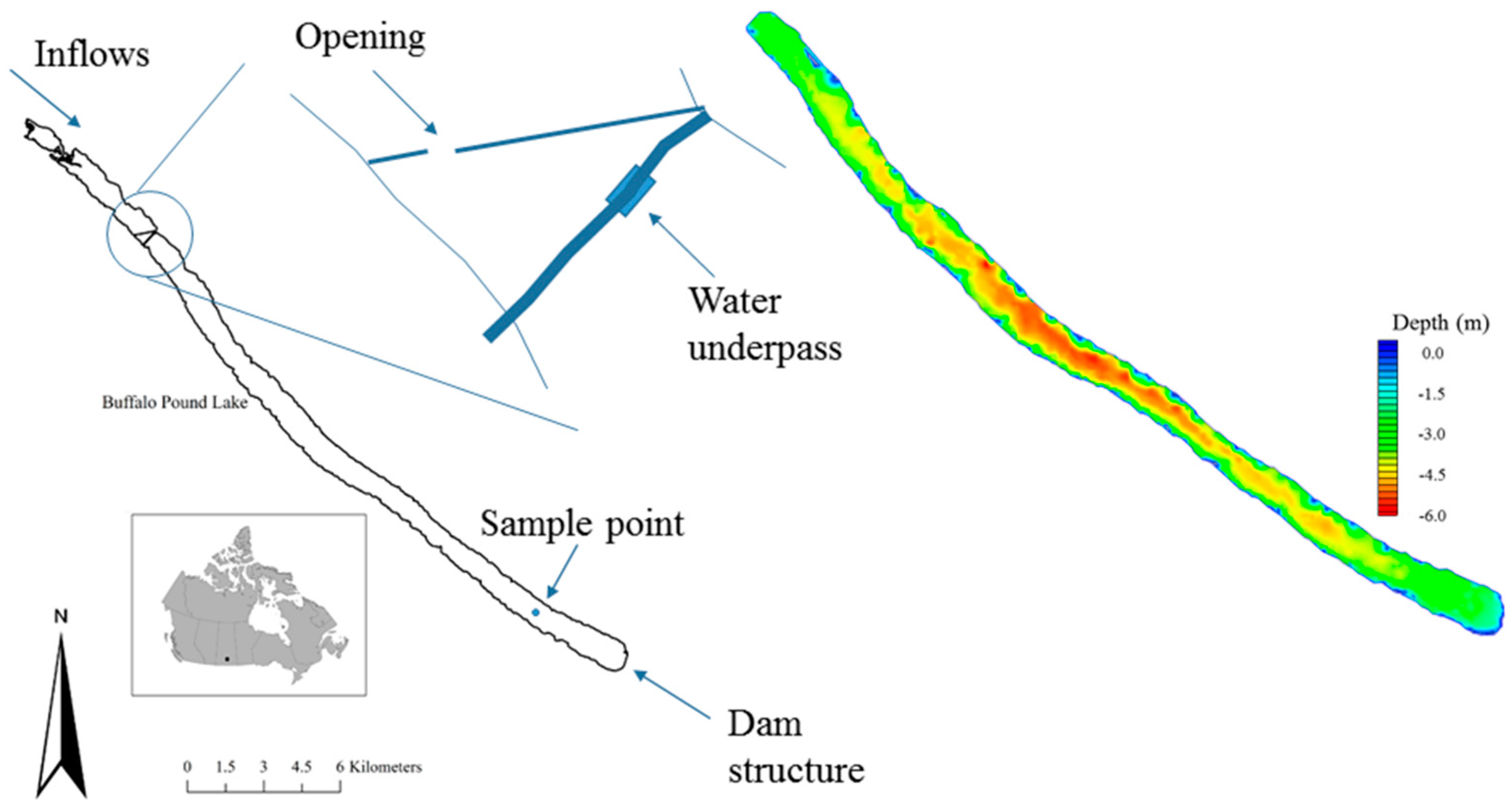
Buffalo Pound Lake (BPL) is an impounded natural lake located on the Upper Qu’Appelle River in the Saskatchewan Province of Canada (Figure 1). The reservoir supplies the water demands of the cities of Moose Jaw, Regina, surrounding communities, and an expanding industrial corridor and potash mines. The reservoir forms part of the glacially formed upper Qu’Appelle River system described in detail in Hammer [24]. Annual mean precipitation is 365.3 mm and approximately 30% falls as snowfall [25]. Ice cover is typically November to late April. Air temperatures range between a daily minimum of −17.7 °C in January to a daily maximum of 26.2 °C in July [25]. Over 95% of the drainage basin is agricultural land [26] suggesting that non-point nutrient sources (diffuse pollution, overland run-off) may factor significantly in nutrient loading to BPL. Water quality issues such as eutrophication remain a challenge, and the reservoir has persistent problems with taste, odour, and algal blooms [27,28].

2.2. Model Setup

W2 needs full geometric data to operate. A digital elevation model (DEM) was prepared in ArcGIS 10.2.2 (ESRI Inc., Redlands, CA, USA). The DEM includes sonar data collected by boat in 2014, and a reservoir extent polygon and shoreline digital elevation data provided by the Saskatchewan Water Security Agency (WSA). The combined GIS data are interpolated using a spline barrier method at 30 m resolution. The Upper Qu’Appelle flows into the northwest end of the reservoir with the dam located at the southeast end. In essence, the upstream area of BPL is split into separate waterbodies by Highway 2, which dams the reservoir down to the reservoir bed (Figure 1). The first obstacle that the inflows meet is the breaker built to protect the highway. Once the flows are through the breaker they are then squeezed through a gap of 45 m (three connected 15 m sections) under the bridge, and into the main body of the reservoir. The top section of the reservoir is extremely shallow and weed choked, and sonar data could not be collected by boat. The top and main body of the reservoir will likely experience some differences in reservoir conditions making it less realistic to model the reservoir as just one waterbody. Water quality data were available for under Highway 2 and so these are set as boundary data. The DEM and water quality model covers the whole main body of BPL downstream of Highway 2.

W2 discretises the waterbody into a finite grid of longitudinal segments, vertical layers and cross-sectional widths. The user specifies the space steps in the longitudinal and vertical directions. The cross-sectional widths are determined by the shoreline bathymetry as each cell spans the width of the waterbody. The prepared DEM has been segmented into a numerical grid in the Watershed Modelling System (WMS) (Aquaveo, Provo, UT, USA) for final output as a bathymetry text file for W2. Longitudinal segments average 100.9 m with a total length for all 256 segments of 25,834 m. Vertical layers are 0.25 m with the maximum number of layers being 26 at the deepest part of the reservoir. W2 requires boundary layers and segments that are all zero meters and these are included in these totals. Average width at the surface is 890 m.

2.3. Data Collection and Analysis

Hourly meteorological forcing data have been downloaded from Environment Canada (EC) for the Moose Jaw station located approximately 30 km south from BPL. In order to estimate the wind conditions at the reservoir surface, comparisons have been made of recent EC data against data from an in situ high-frequency data collecting buoy. This buoy has been deployed on BPL by the Global Institute for Water Security since 2014 for open water field seasons. Snowfall figures are also taken from the EC Moose Jaw station, and are monthly totals. The “snow on the ground” measurement is the physical quantity of snow-cover on the last day of each month.

Gauged averaged daily inflows have been downloaded directly from the EC website. Accurate inflow data is not available for the BPL boundary of Highway 2, and flows are from the nearest gauge 19 km upstream on the Upper Qu’Appelle River. This is land distance—the flows will travel further as the channel meanders. Monthly mean estimates of ungauged inflows are provided by the WSA and include minor tributaries located after the EC gauge, as well as overland run-off estimates.

The main outflows from BPL are dam releases and piped withdrawals. The dam releases have been derived using EC data for two downstream flow gauges. The withdrawal volumes are provided by the on-site Buffalo Pound Water Treatment Plant (WTP) and by SaskWater. Daily averaged water-level measurements are provided by the WSA for an in-reservoir gauge.

Monthly inflow DO and BOD measurements are provided by the WSA for a sample site at the Highway 2 boundary. The in-reservoir observed data are taken from a substantial weekly dataset provided by the WTP laboratory. The WTP weekly samples are normally taken around 07:20 a.m. at a sample site midway between the north and south shorelines near the downstream end of the reservoir, and approximately one meter off the reservoir bed. The reservoir is expected to be well-mixed at the sampling point. Water is withdrawn through an intake pipe at this location to the WTP’s pumping station, on the south shore, where sampling takes place before the water is pumped to the WTP itself. These samples are transported to the WTP laboratory for analyses. This procedure is performed weekly in both open water and under-ice conditions. Some spot sample water quality data are available for other locations across the lake, although not all constituents are measured regularly at these additional sites, and they have not been included in this study.

Weekly inflow temperatures are estimated through a linear regression (R² = 0.861; equation y = 1.0598x − 2.7747; 59 samples; no outliers removed) between WTP spot sample temperature measurements over 34 years at the site of the inflow gauge upstream, and the WTP weekly temperature data for the reservoir. Precipitation temperatures are set at dew-point temperature, or zero if the dew-point is negative.

Initial conditions for water temperature and DO are also taken from the WTP weekly dataset. Sediment temperature is set at the mean annual air temperature over the simulation period as per the W2 manual recommendation [23]. Parameter coefficients are set according to knowledge of the reservoir, or are left at W2 default values where data are not available to support a change. The kinetic coefficients for BOD and SOD are W2 defaults (

Table 1. W2 Default kinetic coefficients used in this study for the sediment oxygen demand (SOD) and biochemical oxygen demand (BOD) calculations.

Coefficient	Description	Value	Units
TSED	Sediment temperature	10.3 1	°C
CBHE	Coefficient of bottom heat exchange	0.3	W·m−2·°C−1
KBOD	5-day BOD decay rate at 20 °C	0.1 2	day−1
TBOD	Temperature coefficient (decay rate)	1.02 2
RBOD	Ratio of 5-day BOD to ultimate BOD	1.85 2
CBODS	BOD settling rate	0.0 2	m·day−1
SODT1	Lower temperature for zero-order SOD or first-order sediment decay	4.0	°C
SODT2	Upper temperature for zero-order SOD or first-order sediment decay	25.0	°C
SODK1	Fraction of SOD or sediment decay at lower temperature	0.1
SODK2	Fraction of SOD or sediment decay at upper temperature	0.99
REAERAT	Reaeration formulation	LAKE, 6

Notes: ¹ Where the value is different to the W2 default; ² W2 uses CBOD as the model group; we are assuming that CBOD makes up the majority of our BOD.

).

For quality assurance, the WTP data span the complete simulation period and undergo strict quality control sample procedures. The flow data, water-level data and meteorological data downloaded from the WSA and EC websites are expected to have undergone quality control prior to commencement of the study. Metadata is available for the WSA water-quality database that details the source and perceived accuracy of the measurements.

2.4. Model Customisation

We have customised two components of the W2 model: SOD and the ice algorithm. This study uses W2 version 3.72, which includes a zero-order, or a limited first-order, sediment compartment for estimating SOD. The latest version of W2 (v4.0) also includes a new sediment diagenesis model; however, with no sediment data to drive a full diagenesis compartment, there would be considerable uncertainty at the large scale of a reservoir. We opted for v3.72 as the complete source code for v4.0 was not available for download on commencement of our study, and we were unable to customise the later version for our specific objective.

W2 uses three different types of data for model calibration: the first group are set prior to the model run and remain constant throughout the simulation—examples being latitude for the calculation of solar radiation, bathymetry, and parameter coefficients. The second group are the time-varying state variables such as inflows, outflows, and meteorological data. The third group are the variables changing internally in the model at each time step; temperature, shear stress, and horizontal and vertical velocities are examples of this group.

DO is calculated in W2 as per Equation (1). The complete set of DO equations in W2 are more complex as the model recognises up to thirteen sources and sinks of DO [23]. We present here the W2 equations we use in our own reservoir DO/SOD model.

$$S_{\mathrm{DO}}=\underset{aeration}{\underbrace{A_{sur}{K}_L\left({\mathsf{\Phi }\prime }_{DO}-{\mathsf{\Phi }}_{DO}\right)}}-\underset{zero-orderSOD}{\underbrace{\mathit{S}\mathit{O}\mathit{D}{\gamma }_{OM}\frac{A_{sed}}{V}}}-\underset{BODdecay}{\underbrace{{\displaystyle \sum }{K}_{BOD}{R}_{BOD}{\mathsf{\Theta }}^{T-20}{\mathsf{\Phi }}_{BOD}}}$$

(1)

where:

$A_{sur}$	$\mathrm{water}\mathrm{surface}\mathrm{area},{\mathrm{m}}^2$
$K_L$	interfacial exchange rate for oxygen, m·s−1
${\mathsf{\Phi }\prime }_{DO}$	saturation DO concentration, g·m−3
${\mathsf{\Phi }}_{DO}$	dissolved oxygen concentration, g·m−3
$\mathit{S}\mathit{O}\mathit{D}$	sediment oxygen demand, g·m−2·s−1
${\gamma }_{OM}$	temperature rate multiplier for organic matter decay
$A_{sed}$	sediment surface area, m2
$V$	volume of computational cell, m−3
$K_{BOD}$	BOD decay rate, s−1
$R_{BOD}$	conversion from BOD in the model to BOD ultimate
$\mathsf{\Theta }$	BOD temperature rate multiplier
${\mathsf{\Phi }}_{BOD}$	BOD concentration, g·m−3

The zero-order SOD is a user-defined constant rate that is temperature dependant. In the original source code the model reads the SOD at the start of the simulation, and uses the same rate in the equation for the whole simulation period. The zero-order SOD is displayed in bold text in Equation (1). In W2, BOD is imported as a time-varying variable in the inflow constituent file. We modified the W2 code to treat SOD in a similar manner and read SOD as a time-varying temperature-dependent input file. The model checks for new values of SOD during each iteration and updates the zero-order SOD in Equation (1). The original constant SOD rate in W2 is now a variable rate in the DO equations, although the DO module itself is unchanged.

For the ice model W2 calculates the formation and melting of ice during simulations, and the relevant processes (e.g., light, wind, heat fluxes) are adjusted accordingly by the model. Snow is not considered in the algorithm. Snow depth at BPL is often between 0.1 and 0.3 m as per the supplied WSA long-term data. To account for this lack of snow the ice model has been extended to include two empirical coefficients to the existing W2 algorithms, as have been previously applied [29]. The first coefficient α extends the ice growth and thickness equations and reduces the heat lost through back radiation from black surfaces. The second coefficient β extends the ice melt equations and reduces the heat conduction between air and ice. Both coefficients are assigned a value between zero and one to be multiplied by the appropriate equation parameter. For BPL, no ice thickness data are available for calibration of α. A 39-year data set of ice-on and ice-off dates has been provided by the WTP, and it is found that W2 predicts the ice-on dates to be closely matched with the observed dates. For this study, the coefficient α is set to have no contribution to the ice growth equation (given the value 1). Ice-off dates were difficult to match as the ice melts too quickly in the W2 simulations—up to a period of several weeks. The optimum value of coefficient β is found to be 0.24 to predict the best spring ice-off dates over the simulation period.

2.5. Model Setup and Application

The model simulates a continuous seven-year period (1 April 1986–31 March 1993). This period is chosen due to the availability of daily flow data recorded by two WSA gauges just above and below BPL that were subsequently discontinued.

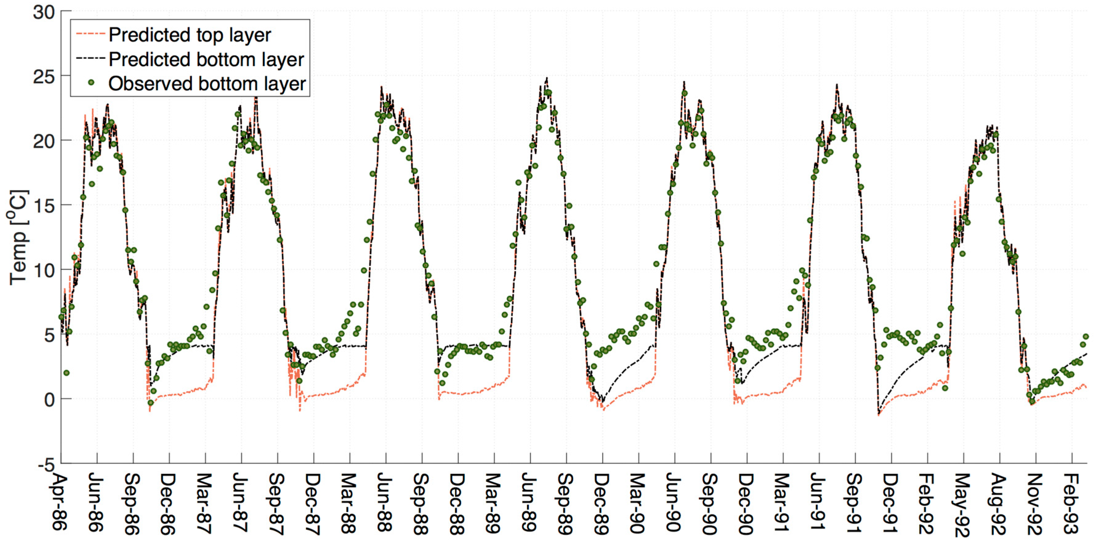
The water balance, ice-on and ice-off dates, and the water temperature model were calibrated. The final temperature model shows good results (Figure 2). Some discrepancy occurs in the winter of 1989/90 and 1991/92 with the model under-predicting the winter bottom temperature and possibly the stratification. The temperature profile can depend on the meteorological conditions at freeze-over. In addition, many of the temperature sensitive parameters and coefficients in W2 (e.g., sediment temperature, bottom heat exchange, surface albedo) are fixed in the model. It is likely that there is some temporal variance in these in-reservoir.

The monthly ungauged inflow estimates provided by the WSA are created to close their own water-balance for BPL, and our respective water-balances differ as a result of methodology and data. We chose not to use the provided estimates due to the uncertainty. Another limitation is that the downstream flow data, which we have included, have room for error due to the presence of wetlands, and the potential for backwater flows during the freshet from a tributary confluence downstream of the reservoir. To close our water-balance we have incorporated a distributary tributary (DT) using the W2 in-built water-balance tool. The total contribution of the DT flows is approximately 1.4% of total inflows and precipitation over the eight-year simulation period, although there are seasonal fluctuations. An exception is the winter of 1992/93 where the maximum contribution of DT flows to total inflows under ice reach 22%. This is likely due to uncertainty attributed to error in the withdrawals to the industrial corridor as they are reported on yearly totals. These final year DT flows equate to an approximate 6.5% of BPL volume based on our initial reservoir volume in the DEM (BPL water levels are controlled within a few cm). We aim to assign the DT flows to ungauged inflows and/or outflows once we calibrate the full water-quality model—based on our chemical and nutrient data. For this study, we are assuming that constituent concentrations are primarily introduced in the main river inflows, and that DO and BOD inputs are zero in the DT flows.

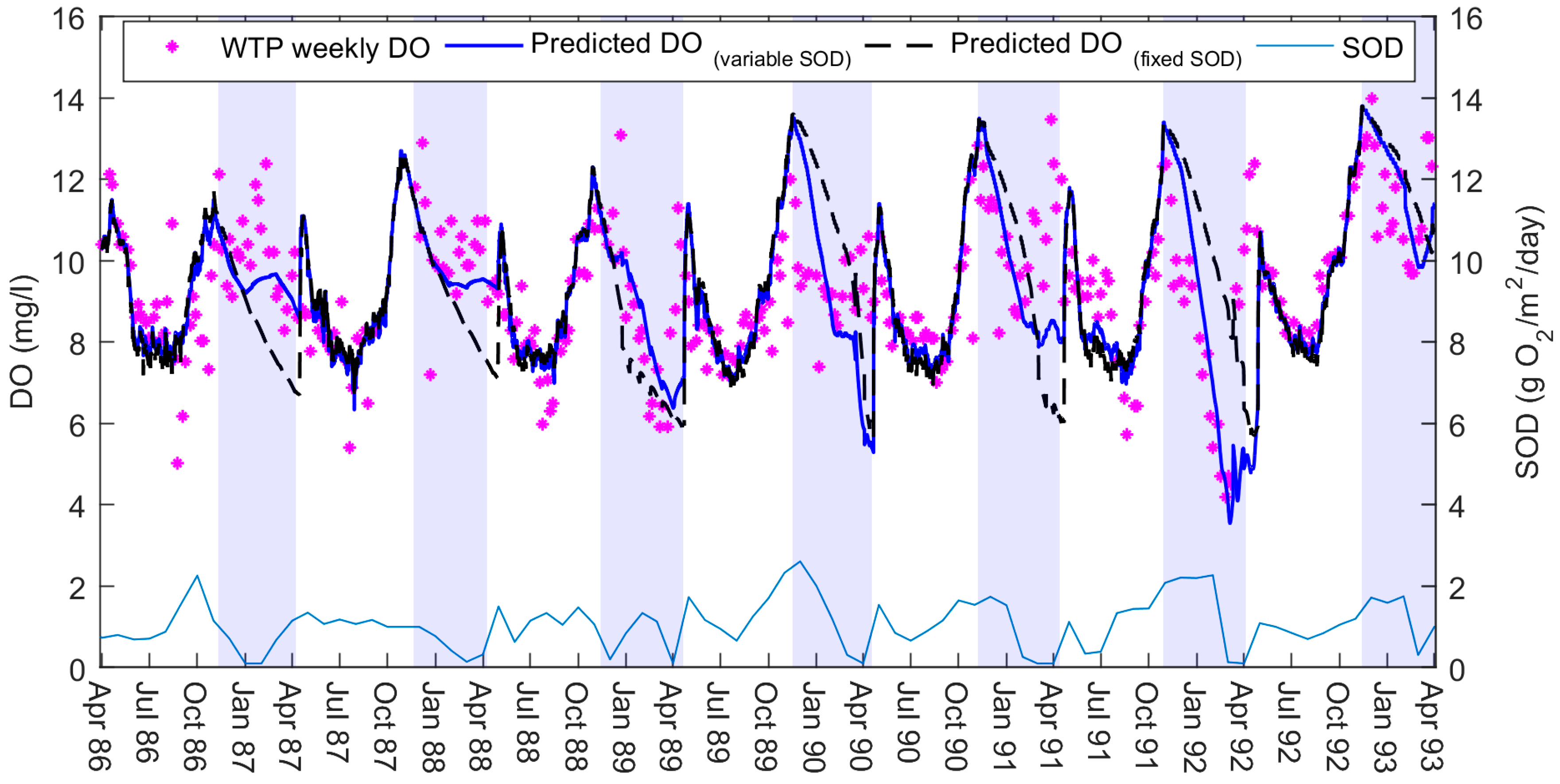
We first simulated a simple DO model of BPL with a constant SOD, for comparative purposes. We extended the calibrated temperature model by enabling the water quality variables DO and BOD (BOD as one group) in W2. We proceeded to calibrate the SOD rate as part of a Monte Carlo analyses for several coefficients. We used MATLAB (MathWorks, Natick, MA, USA) to run W2 for these calibration iterations and attempted to fit the predicted DO to observed DO concentrations. Using a constant SOD we were only able to produce a moderately good fit (Figure 3): with both underestimations and overestimations of DO throughout the simulation period.

To introduce a variable SOD we took the DO model of Figure 3 and implemented a semi-automated calibration through MATLAB. The code attempted to match W2’s predicted DO to the observed data by changing the SOD at weekly intervals. We used simple rules: for each weekly period, if the predicted DO concentrations were overestimated then the MATLAB code increased the SOD to increase consumption. If the predicted DO concentrations were underestimated then the SOD decreased that week. All weeks were changing simultaneously during the iterations and we ran the model until the SOD rates reached a stable condition.

We found that the DO model performed better with the variable SOD rates (Figure 3). On examining the results of this new model, we noted that SOD followed a relatively consistent seasonal trend. SOD was high over summer, peaking towards the end of the season, and then gradually depleting over winter. The rates of SOD were different in magnitude each year, yet similar in behaviour.

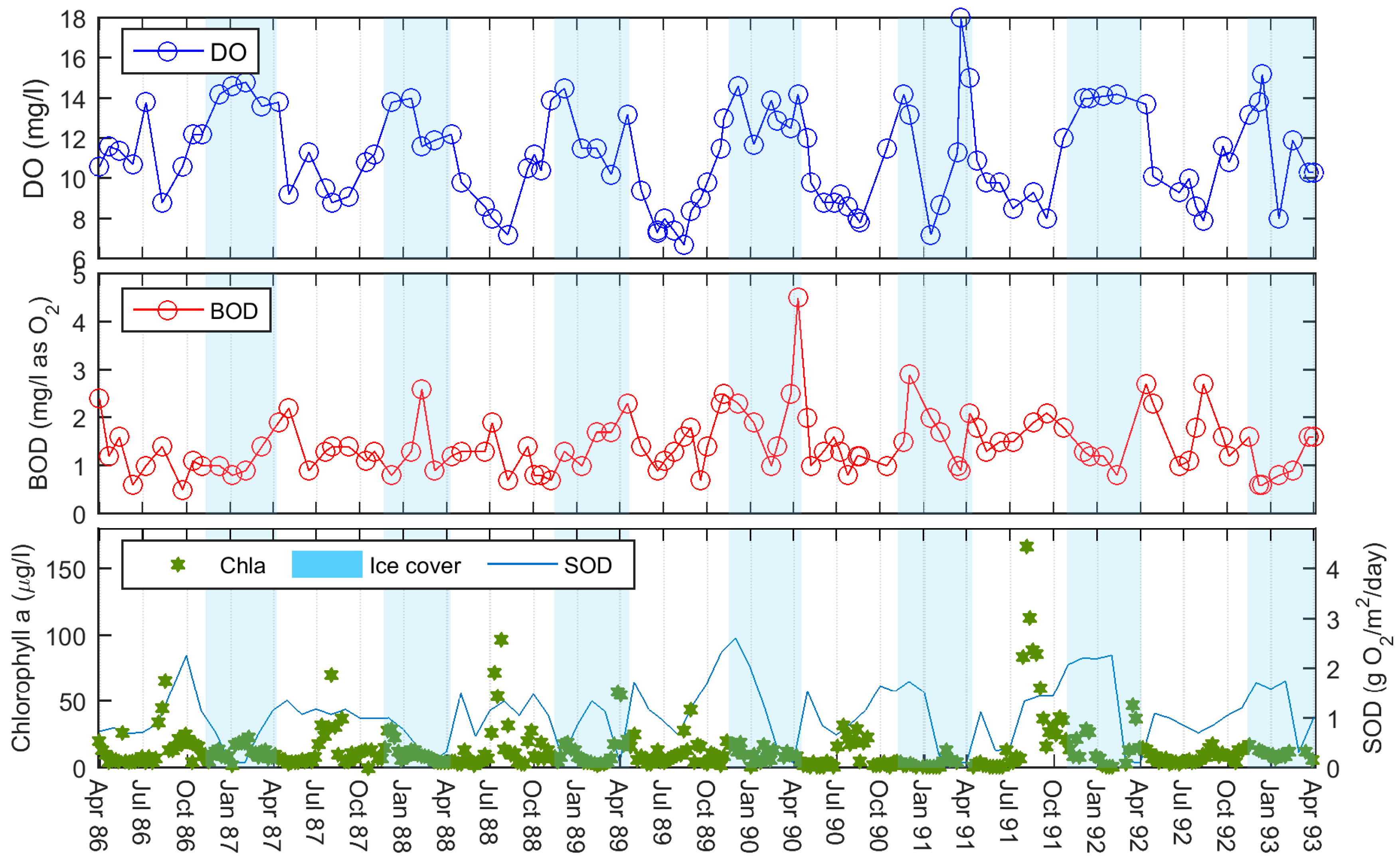
We compared the new SOD results against observed in-reservoir water-quality data to look for trends. We noticed that the predicted SOD appeared to follow a similar pattern to the observed weekly summer chlorophyll-a (Chla) concentrations (Figure 4) over the first few years: with SOD peaking not long after Chla. In light of this, we investigated if any relationships could be found between Chla abundance, and SOD. Our aim was to determine if Chla might be useful as an alternative measurement for estimating SOD. We approached the open water and under-ice periods differently due to the restriction of ice-cover on reaeration. We wanted to maintain the assumption of having limited data with which to build a model, and we aimed for simple strategies.

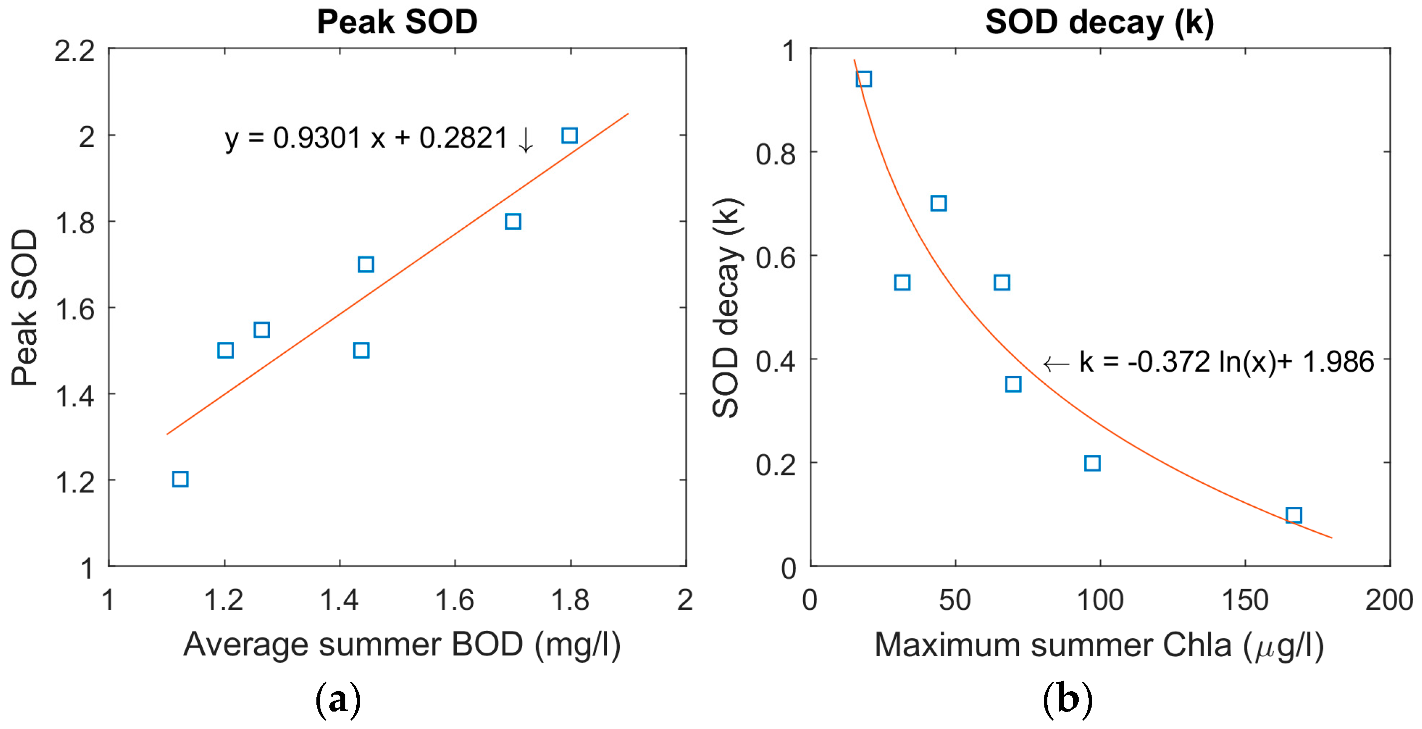
For open water seasons reaeration can replenish oxygen as it consumed, and we elected to keep our SOD constant over these periods. We allowed the model to have interannual variability by using individual SOD rates for each year. We began by averaging each summer variable SOD presented in Figure 3. Taking these averages, we found that the lowest and highest seasonal SOD occurred in the respective years of the lowest and highest maximum summer Chla concentrations in the reservoir. This made it simpler to assume the two SOD values as being our SOD range. We then used an equation based on the apparent relationship of these two variables (summer SOD = 0.0042 × max summer Chla + 0.9345) to set the remaining summer SOD rates based on the maximum summer Chla concentrations each year. By this method, we used the previous summer’s maximum Chla concentrations as a proxy of the magnitude of biomass production that settled to the bottom sediments by the end of the open water season.

To simulate end of season algal bloom mortality and winter decay we again used MATAB to adjust the SOD rate, so that predicted DO fit to observed DO, from one-month before ice-on occurred until ice-off the following spring. We implemented the same weekly semi-automated calibration process as before, and the SOD rates generally peaked before the ice-on event. Under ice-cover W2 automatically stops any gas exchange, and reaeration equals zero. This allows us to imitate a first-order decay rate during this time.

Once we had both the end of season peak SODs and winter SODs we were then able to back-calculate the winter SOD decay rates (k) for each year based on Equation (2):

SOD = peak SOD × weeks^−decay(k),

(2)

where the predicted winter SOD in W2 is assumed to be a function of the predicted peak SOD, and the number of weeks since the start of ice-cover to the decay rate k; With k being the unknown in this equation. These back-calculated decay rates were then plotted against summer Chla.

3. Results

3.1. Dissolved Oxygen Simulation

The final DO model shows good overall results (Figure 5). The predicted DO observations follow the pattern of the observed DO measurements in most years. There is some underestimation in the winters of 1986/87, 1987/88 and 1992/93. SOD follows a similar trend for each year with an end-of-season peak, and winter decay. The SOD remains high in the winter of 1991/92 due to a greater than average oxygen depletion that year. There is a clear connection in the model between the predicted DO, and the observed ice-on and ice-off dates provided by the WTP.

3.2. Sediment Oxygen Demand Relationships

The peak SOD does not fit particularly well with the maximum or average summer Chla. Interestingly, in comparison with observed data for BPL, the peak SODs appear to have a high correlation (R² = 0.85) with the average BOD inflows included in our model for the open water period. (Figure 6a). The winter SOD decay rates have a negative, exponential relationship with both the average and maximum summer Chla concentrations of the previous summer. The relationship between SOD decay and the maximum Chla (Figure 6b) is slightly stronger at R² = 0.88 (average Chla: R² = 0.84).

4. Discussion

A zero-order approach for SOD that treats the demand as an input variable rather than a calculated one does not reflect the conversion of organic matter settling during the simulation [10]. Our original intention was to allow the model to find the changing SOD values through matching to observed DO concentrations. For this, the model was calibrated in MATLAB using a semi-automated iterative process that allowed the model to change the SOD weekly. The resulting SOD values were then to be read by W2 as an input file; this would imitate a first-order compartment, in essence, by varying through the simulation. The model indeed predicted DO concentrations more closely with this variable SOD file than with the W2’s original fixed rate option.

Calibrating the SOD with the purpose that the model’s DO predictions match with observed DO measurements can be an unsound technique as it assumes that other parameters such as reaeration and settling rates are already well-known [11]. This method of calibration also combines several reservoir processes that contribute to DO into one net value that is assumed to be SOD. While these points suggest that there are limitations to this approach, there remains the problem that few aquatic managers have sufficient data available to run the full diagenesis model. In view of this, we assessed the initial results to see if there were other trends that matched what we know about BPL, and that might suffice as a proxy measurement or explanatory variable.

The reservoir is a highly eutrophic system with high incidences of algal blooms. Deoxygenation can occur after the collapse of a summer algal bloom due to additional bacterial activity [2]. In general, the more enriched the system then the higher the rates of productivity and ultimately the greater the oxygen depletion from decomposition [3]. Chla has previously been used as a proxy for estimating in-lake BOD [30]. Based on this principal, and our knowledge of the reservoir, we are assuming that most of the autochthonous contributions to oxygen demand within BPL are related to algal activity (apart from nitrification and chemical oxygen demand). Any allochthonous inputs to oxygen demand are already included in our BOD time-series data in the inflow constituent file—with the caveat that we are using the W2 default BOD settling rate between upstream and our sample site on the reservoir.

We have found this approach to be successful, as shown in Figure 5. The summer SOD rates based on a correlation with the summer Chla concentrations act effectively as a substitute to our weekly variable SOD. This suggested link between oxygen depletion and productivity also agrees with our findings relating winter SOD decay to the Chla concentrations of the previous summer. This is noticeable in the results for the winters of 1988/89 and 1991/92 where the SOD remains high under ice-cover following large summer algal blooms.

In contrast, a result of no correlation between Chla and DO consumption is found in other shallow prairie lake sites [3]. The study in question suggests that the most important predictor of DO consumption is macrophyte biomass due to the large contribution to particulate organic matter (POM). This is found to be also true in sites with abundant phytoplankton, although the authors point out that the algal-derived carbon averages 150 times less than the macrophyte-derived carbon in their study. In BPL, apart from the top section outside of the model boundary, the reservoir is not thought to have many macrophytes. This may explain why we are able to find a relationship between summer Chla and winter SOD decay as the macrophyte contribution to POM is not important in this reservoir.

Our winter SOD decay pattern declines in an exponential manner with a rapid reduction at the onset of winter. This theory fits with the suggestion that the first three months of ice-cover have the greatest oxygen consumption due to the rapid oxidation of certain organic materials over others, for example [31].

The apparent connection between peak SOD and the average BOD inflows for the open water season is more surprising as we had suspected that the low values of BOD would have little impact in the reservoir. SOD and BOD are, in fact, often combined into one demand known as hypolimnetic oxygen demand [18]. In an ideal model BOD and SOD would be kept separate. Our internal BOD is included with our SOD, as is reaeration. In addition, BOD inflows are based on monthly samples. The result is that we cannot ascertain for certain the relative importance of BOD flowing into the reservoir.

In the winters of 1986/87 and 1987/88, the model under-predicted the DO concentrations. However, in these years, it can be seen that although snowfall was still high in both years, there was little snow left on the ground at the end of each month. It is possible that the reservoir winter albedo is relatively low in these years and light can penetrate the ice to allow photosynthesis to take place. This is evident in the observed winter Chla concentrations (Figure 4). This is a winter phenomenon that we are unable to capture in the model as we do not simulate primary productivity, and our SOD equations are founded on summer Chla. While snow on the ground is also minimal in the winter of 1991/92, this year is different as the intense summer algal bloom preceding this year results in the DO concentrations falling and the SOD remaining high.

What is interesting in the winter of 1992/93 is that the snow cover is high throughout the winter, suggesting low light availability, and yet DO concentrations are high. On examination of the temperature model (Figure 2), it can be seen that the observed bottom water temperatures are much lower in this year than in previous years. Cold water holds more oxygen than warm water [5], and estimating DO inputs based on monthly samples may be missing occasional elevated DO concentrations in cold river inflows during periodic snowmelts. The winter of 1992/93 also has the greatest contribution of the distributary tributary inflows, which indicates that there may be a larger amount of ungauged inflows contributing to the water balance in W2 with no corresponding DO input file.

Another point to consider is that oxygen consumption rates are shown to be temperature dependent with lower consumption rates at lower temperatures [12]. Both the summer temperatures of 1992 and winter temperatures of 1992/93 were colder than previous years. This suggests that less heat may be stored in the sediments. The sediment temperature in W2 is a fixed user parameter, and in our model has been set at the average annual air temperature over the simulation period (where temperature >0 °C). The observed sediment temperature may be colder than this average value in the final winter, and, in reality, the sediment oxygen requirements are lower than we are modelling.

An equation for the effect of water temperature on SOD shows how temperature and SOD have a positive relationship with each other: SOD starts to decline more rapidly after temperatures go lower than 10 °C, and reduces towards zero as water temperatures drop below 5 °C [11]. Part of the pattern of SOD changes in BPL will also be a function of bottom water temperature. Our SOD decays rapidly to near zero levels quite early in the colder water temperatures of winter 1992/93. The temperatures in BPL are fairly consistent year-on-year until the summer of 1992, and the winter decreases and summer increases of SOD in response to temperature are expected to be comparable up to this point. This leaves Chla explaining the SOD variance between the individual years.

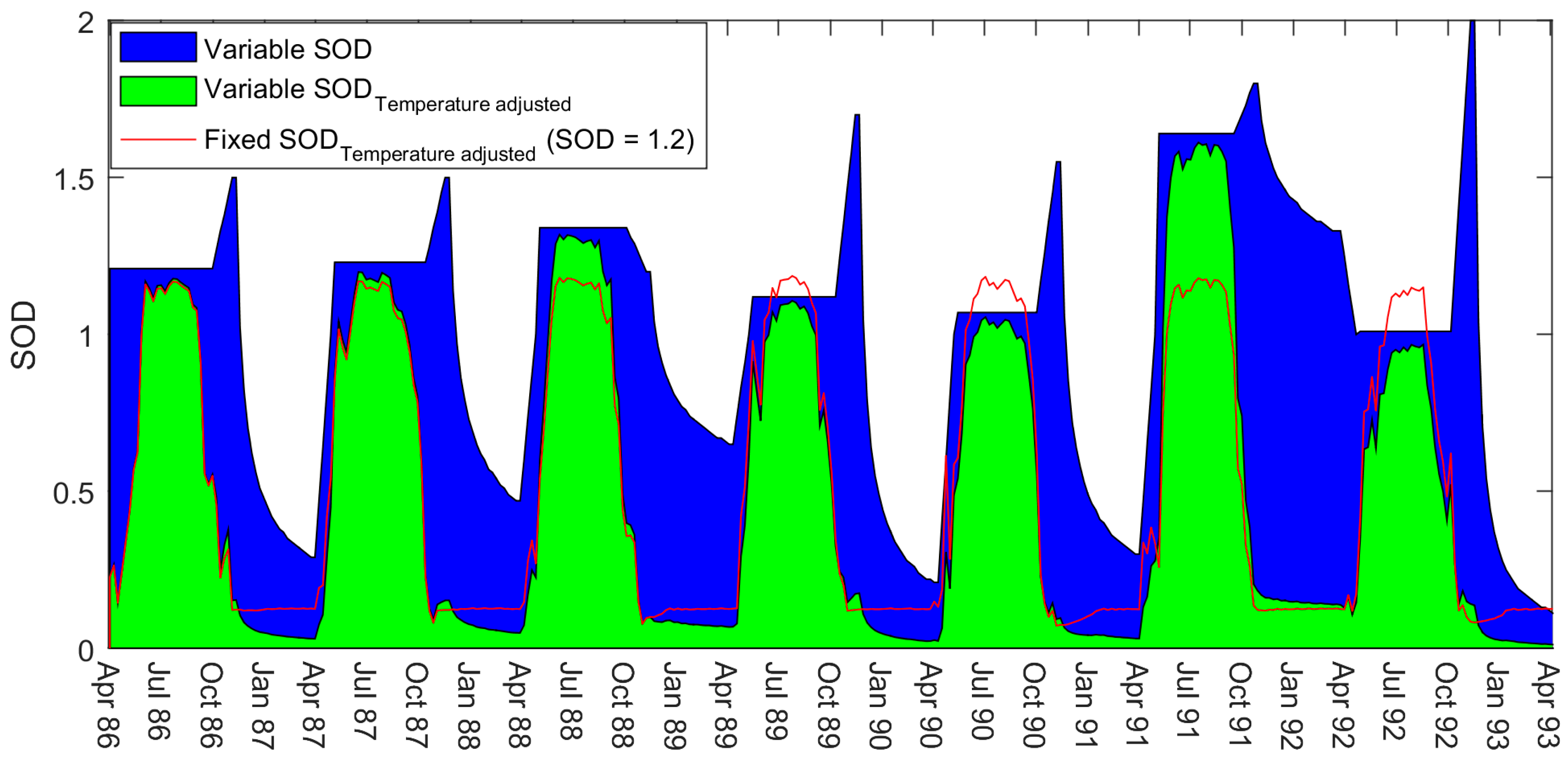
W2 uses four SOD temperature-rate multipliers to adjust the rate of SOD decay as a function of temperature in the model. They are model calibration parameters, and can be helpful in reproducing the changing rate of consumption of DO. We have used the default settings in W2 (Table 1). The variable SOD values that we include in W2 as an input file are maximum SOD rates—the same as the model format for a constant SOD rate. Figure 7 shows the temperature adjusted rates that W2 is actually using during the simulations based on these default calibration parameters. A contributing reason for the end of summer SOD peaks, for example, might be that the rapid decreases in the temperature adjusted SOD are too extreme. The model may potentially increase the maximum SOD to compensate for this temperature effect when calibrating SOD to match the predicted DO with observed DO. We had no data with which to justify changing the default values. Likewise, we did not wish to increase our model uncertainty by expanding the number of parameters with no additional data. We instead chose to adjust just one parameter (SOD) for our purposes.

There are a few differences between SOD found by using MATLAB to vary SOD each week to fit the predicted and observed DO to each other (weekly model—Figure 3), and SOD found through basing the demand on summer Chla (final model—Figure 5). The winter decay in the final model agrees well with the drops in SOD in the weekly model except for the winter of 1991/92. In this year, the weekly model drops the SOD to zero when the DO levels are extremely low and then increases SOD as the oxygen levels rise. This is the opposite behaviour to what we would expect in a limnological sense. The behaviour of the final model in this time period is more realistic. The relatively large peak in SOD at the end of this summer may possibly be due to the BOD inputs being higher this year (Figure 4).

In reality, the rapid peaks in SOD shown in Figure 5 are also likely a result of our holding the SOD at a constant rate over the summer period. The final model uses average summer rates, and will miss some of the variability that would naturally occur. In the semi-automated calibration of Figure 3, we show that when the model uses variable weekly SOD rates there is a general (with some fluctuations) increase over the course of the summer. This agrees with our assumption that SOD in BPL cumulates to a peak due to biota dying towards the end of the season. By holding the model at an average seasonal SOD, instead, we are likely overestimating the SOD in spring, and underestimating the SOD in autumn—if we are to assume that SOD increases as suggested by Figure 3. We found that our winter decay relationship with Chla was stronger if we allowed MATLAB to adjust SOD so that the predicted DO fits to the observed DO at the onset of ice-on. In order to achieve this, we had to release the model from the fixed SOD rate at the end of the season—thereby simulating the end of season peak. We chose a one-month period prior to ice-on as a sensitivity analysis showed that this gradient of SOD adjustment gave us the best overall results for summer and winter.

This summer averaging method is most likely responsible for the sudden increase in SOD at ice-off in April. There will be natural processes leading to an increase in SOD (e.g., warmer water, spring blooms, and spring turnover) that will be exaggerated by the need for the SOD to instantly increase to the average summer rate at the start of spring. Other methods may be to allow the model to increase gradually over the whole summer duration, either linearly or exponentially, although we would need to consider some way of verifying the manner in which it increased. Our strategy was to approach the problem as if having little to no data to verify the predicted SOD rates (except using DO data). We decided to constrain the model to using an average summer rate based on a relationship found with Chla, and then allow the SOD to decay over winter dependent on a fixed equation. Thus, the aquatic manager would only need to find (and ideally verify) limited points, such as the end of season peak rate, rather than weekly SOD rates.

One limitation to our study is the disconnection between the top and main section of the reservoir. While our inflow constituent file is based on observed data from under Highway 2, and the boundary of our model, the inflows themselves relate to a gauge further upstream on The Upper Qu’Appelle River. It is uncertain at present what effect the top section of the reservoir, the wave-breaker, and the 45 m gap under the highway have on our inflow boundary data.

Finally, while our extended W2 ice model is a suitable model for seasonally ice and snow-covered waterbodies, the W2 model has a fixed albedo coefficient through the simulation. The extension to the ice model stops the ice melting too quickly by keeping the snow on the ground, yet does not help with modelling the correct amount of light penetrating the ice. This will make it difficult to calibrate DO, when primary production is added to the model, with just one value for high and low snow years, and different ice structures. This is due to the influence of light on photosynthesis and oxygen production, as indicated in the observed data in the winters of 1986/87 and 1987/88. Our future plans include modifying the ice model further to include a function for a variable albedo. We think that this will be an interesting step to take forward and is a missing-link in modelling DO/SOD relationships in ice-covered reservoirs.

5. Conclusions

From the modelling, we show that winter SOD decay is inversely dependent on the previous summer’s maximum Chla concentrations. The decay rate is faster when less algae are produced. A constant SOD value suffices during the summer half-year; however, a better DO simulation is obtained in winter when the SOD rate decays during the course of the winter. This implies that the biomass supply during winter is limited and much of the draw on DO is diminished by the end of the winter. This result is backed by several field studies. We have shown that for a Prairie shallow reservoir with few macrophytes and BOD inputs variable SOD can be used in a water quality model to represent additional oxygen demand after an algal bloom. The summer SOD and winter SOD decay can be estimated by treating the open water and under-ice period individually in the model. This variable SOD over-time can be estimated for both summer and winter conditions based on summer concentrations of Chla. This concept can be widely applied to similar systems that do not have data to support a full diagenesis model, yet would benefit from a more representative estimation of SOD than is provided by a zero-order constant SOD rate.