
Integrating Local Scale Drainage Measures in Meso Scale Catchment Modelling


Institute of River and Coastal Engineering, Hamburg University of Technology, Denickestrasse 22, 21073 Hamburg, Germany
*
Author to whom correspondence should be addressed.
Water 2017, 9(2), 71; https://doi.org/10.3390/w9020071
Submission received: 12 September 2016
/
Revised: 23 December 2016
/
Accepted: 30 December 2016
/
Published: 25 January 2017
(This article belongs to the Special Issue Hydroinformatics and Urban Water Systems)
Abstract
:This article presents a methodology to optimize the integration of local scale drainage measures in catchment modelling. The methodology enables to zoom into the processes (physically, spatially and temporally) where detailed physical based computation is required and to zoom out where lumped conceptualized approaches are applied. It allows the definition of parameters and computation procedures on different spatial and temporal scales. Three methods are developed to integrate features of local scale drainage measures in catchment modelling: (1) different types of local drainage measures are spatially integrated in catchment modelling by a data mapping; (2) interlinked drainage features between data objects are enabled on the meso, local and micro scale; (3) a method for modelling multiple interlinked layers on the micro scale is developed. For the computation of flow routing on the meso scale, the results of the local scale measures are aggregated according to their contributing inlet in the network structure. The implementation of the methods is realized in a semi-distributed rainfall-runoff model. The implemented micro scale approach is validated with a laboratory physical model to confirm the credibility of the model. A study of a river catchment of 88 km2 illustrated the applicability of the model on the regional scale.
1. Introduction
Globally, more than 50% of the world’s population lives already in urban areas. This proportion increased from 30% in 1950 and it is projected to be increased up to 66% in 2050 [1]. This situation poses an increasing stress on the urban environment, infrastructure and water management. Various water system components (i.e., stormwater and sewerage drainage, wastewater treatment, rivers and ditches) have to be managed accordingly in a holistic way.
1.1. Numerical Model Review
Models are playing an increasing role in water management to study these highly complex systems in urban and rural areas [2,3]. The recent development in modelling the interactions between urban water system components is reviewed in e.g., [4]. Integrated models are likely to play an important role in the future by combining individual software packages: e.g., catchment or rainfall-runoff, hydrodynamic, water treatment, flood and/or risk models. To achieve an overall sustainable water system, the knowledge and the ongoing development of these submodels (e.g., Rainfall-Runoff Models = RRM) is required.
RRMs are catchment models in which individual components of the hydrological cycle are represented by interconnected conceptual elements [5]. Current RRMs are classified according to their complexity ranging from empirical methods (e.g., curve number method) to conceptual semi-distributed model approaches and fully-distributed hydrological models [3,6]. All these models conceptualize the “real” processes using sets of mathematical equations.
Selecting the right model requires understanding the objectives and the system being modelled [3,7,8]. Although there is a tendency to use more and more spatially distributed model approaches, the conceptual semi-distributed models do not lose their importance in practical application [3,9]. A high spatial heterogeneity and complexity of the catchment requires an adjustable data management according to available spatial data. Geographic information system (GIS) functions play an important role in this context [10]. Conceptual semi-distributed models are likely to be build up with an adjustable data management. This type of model may use different spatial model resolutions within one model setup: rougher model resolution for less heterogeneous spatial areas and a finer model resolution for more heterogeneous spatial areas.
Further on, it is necessary to assess the level of required physical based approaches in the model for specific purposes. It can be stated that the overall individual physical processes in a catchment are still not thoroughly understood in detail and there is still research required to completely understand the interaction between the processes. Using fully-distributed models on the basis of the overall currently known physical approaches may not lead to the best solution for all modelling purposes (e.g., regarding model performance and required data processing).
1.2. The Scale Issue in Numerical Models
The heterogeneity in space and the variability in time are defining features in hydrological science. Heterogeneity describes the diversity of properties in space which define the characteristics of a catchment (e.g., soil properties, surface conditions). The term “variability” is used for fluxes or state variables (e.g., runoff, soil moisture, vegetation cover) which vary in time and/or space. The differentiation of these terms is defined earlier, e.g., in [11]. Hydrological processes occur at a wide range of scales: from local diverse surface covers (e.g., of garden plots or detached housing) of some square meters to monoculture farming of thousand square kilometres (= heterogeneity in space) and from flash floods of several minutes duration to flow in aquifers over hundreds of years (= variability in time). In recent research, scales in hydrological systems are redefined [12,13,14]. One of the main reasons is the availability of more detailed topographical and geographical data. Especially in urban areas the heterogeneity in space is high. The characteristics of the hydrological systems are more complex: for example, considering shapes of buildings and infrastructure of urban areas and the implementation of decentralized stormwater management systems on the local scale of properties.
1.3. The Example of Local Scale Drainage Measures and the Deficits in Numerical Models
In the practice of stormwater management, a change from large scale measures to local scale decentralized drainage measures is recognized. The terminology to define these practices and principles in urban stormwater management became complex [15]. Different terms are used according to the international origin and nuanced definition: low impact development (LID; North America, New Zealand), sustainable (urban) drainage systems (SUDS; UK), water sensitive urban design (WSUD; Middle East and Australia), best management practices (BMPs; United States and Canada), alternative techniques (ATs; France), green infrastructure (GI, USA) [15]. In Germany, the term: “Dezentrale Regenwasserbewirtschaftung” (DRWB, meaning: decentralized stormwater management) was developed during the 1990s (see e.g., in [16]).
The intention of the concept presented in this article is to improve the integration of local scale drainage measures in catchment modelling. The issue of scaling is an important matter in the context of the presented work, but it is not inherent in the previous definitions (e.g., SUDS, LID, BMPs). The focus is set on presenting a concept and its implementation to integrate the modelling of different scale data objects in one model. Therefore, a new term is defined to point out the focus on the scale issue, namely the integration of “local scale drainage measures” (LSDM) in meso scale catchment modelling.
LSDMs are measures spatially defined within the boundary of sub-catchments. The smallest scale of these measures ranges down to some square meters. To assess their performance and corresponding hydrological system components in urban areas under future conditions (e.g., more frequent high storm events), the spatial and temporal scale in hydrological models has to be reasonable small to represent the heterogeneous characteristics. Some progress is realized in incorporating features to model LSDM with different kinds of RRM, but there are still areas for further development, including the integration of local scale hydrological measures on a catchment scale [17].
The deficits in current hydrologic catchment models to simulate the effectiveness of LSDM include the following issues: (1) the model is intended to be developed for large drainage areas; (2) it is mainly developed for flood modelling (derived by large storms); (3) it is based on lumped parameters, which do not allow individual setup and precise placement of local stormwater management measures; (4) it shows weak soil water modelling; (5) it shows weak representation of physical phenomena; (6) it shows a lack of GIS or/and user-friendly interface [17,18,19,20]. These deficits illustrate the need for improved understanding of how local scale drainage measures can be addressed on the catchment scale in numerical models [18,20].
The spatial location of LSDM in current hydrologic models is improved by integrating GIS tools [18]. The spatial scale and location of LSDM in distributed hydrological models (e.g., UrbanBEATS, Multi-Hydro [21,22]) are based on the determination of suitable “block” or “cell” sizes according to the model setup, but may be limited to define one type of measure per simulation run (e.g., one type of green roof, cistern, etc.). The distributed approach with constant cell sizes and limited variation of drainage type definitions is considered to be not flexible enough to model the hydrological processes in catchments with diverse characteristics, e.g., urban catchments with partly dense heterogeneous urbanized areas and partly homogeneous extensive rural areas.
Model approaches supporting a specific number of predefined drainage measure types with a limited layer and material setup are not considered to be adaptive enough for modelling upcoming drainage technologies. A current point of interest in research and application studies is the assessment of the effectiveness of drainage measures with new developed designs. An overview of current designs is given in [23]. The purpose of this article is to illustrate a method to integrate a variety of LSDM types with a modular setup in catchment modelling.
1.4. Outline
A methodology is presented to handle the heterogeneity in space and the variability in time of hydrologic systems in a multiscale approach. The purpose is to apply the parameters on an adjustable spatial resolution within one model setup to integrate local scale drainage measures (LSDM) in catchment modelling. A prerequisite to model LSDM is the definition of features of upcoming technologies in this field described in the following Section 2.
The developed methodology presents three new approaches: (Section 3.1) a data mapping procedure of local scale spatial data objects (so called “overlays”); (Section 3.2) an approach to model interlinked network elements on multiple scales with water storage, water redistribution, exceedance flow control and rainwater harvesting functions; and (Section 3.3) a multiple interlinked layer approach on the micro scale to enable the modelling of upcoming drainage technologies, where backwater and exceedance flow play an important role in the interaction of multiple layered systems.
The important result of the developed methods is the definition of parameters and computation procedures on different spatial and temporal scales. The method makes it possible to zoom into the processes (physically, spatially and temporally) where detailed physical based computation is required and to zoom out where lumped conceptualized approaches are applied.
The implementation into a well-established RRM is presented, which was applied for a catchment study to analyse the effectiveness of LSDM for flood peak mitigation. The implemented multiple interlinked layer approach is validated with a laboratory physical model. It is concluded that the presented and implemented methods improve the way of integrating local scale drainage measures in catchment modelling.
2. Theoretical Approach
The theoretical approach to integrate local scale hydrological measures in catchment models is based on multiscale modelling. It is exemplified by local scale drainage measures (LSDM) integrated within catchment models. A prerequisite to model LSDM is a study of important features of upcoming technologies in this field.
2.1. Multiscale Modelling
To solve problems which have features on different scales of time and space, a so called multiscale modelling is applied [24]. With this approach, the system behaviour on one scale is computed using parameters and numerical formulations from other scales. Each scale addresses a phenomenon over a specific window of length and time. Therefore, particular approaches are required to define the system. On a local scale, numerical models may represent physical processes in more detail whereas meso or regional scale models provide averaged values for the overall sub-catchment or catchment. The definition of scales in literature vary significantly and therefore clear definitions are required [13]. The definitions of spatial and temporal scales used in the presented work are depicted in Figure 1.
The catchment boundary of a water system is defined on the regional scale (>10 km). The water system components (e.g., the drainage systems) are defined on a meso scale (1 km2 to 10 km2) in sub-catchments. On the reach scale, ranging from 0.5 km2 to 1 km2, the preferred flow paths are defined. On the local scale the flow and retention processes of drainage measures like in LSDM are represented. The size of these drainage measures ranges from 1 m2 to about 100 m2. The spatial micro scale is used to represent processes on a small size (<1 m2) like the soil water regime in different soil layers and vegetation processes. The spatial and temporal scales are independently defined. The temporal scales range from the analysis of rapid events like after local heavy rainfall events in less than an hour to seasonal impacts within 1 year to long term effects over 50 to 100 years. Physical processes, like the infiltration and exfiltration processes in the soil, are determined in even smaller time scales of seconds.
The smaller the spatial and temporal scale is defined, the more detailed geographical and process data are required. A model with such a high resolution in spatial and temporal scales is defined with a more complex structure and the number of parameters is increased to specify the numerical system. Parameterization aims to define an adequate set of parameters to specify the system being modelled on the basis of measureable system parameters (e.g., pore volume, layer thickness) and non-measurable system parameters (e.g., land use characterization). Thereby, non-measurable parameters induce a calibration process to obtain a model reproducing simulation results comparable to observed hydrological data. With an increased number of non-measurable system parameters, the model is calibrated on the basis of relatively less measureable information and parameters. Consequently, processes may remain undefined and the developed RRM may show poor predictive capabilities as described in [25]. This phenomenon and risk in model structures is referred to as “over-parameterization” (see [25]). One way to deal with this phenomenon is the definition of a moderate and flexible spatial distribution of parameters, which demands for multiscale model approaches. The aim is to model catchments with an adjustable spatial and temporal resolution of parameters within one model setup. For instance, dense urbanised districts are modelled with local scale parameters, whereas more extensive homogenous rural areas are modelled with meso scale parameters.
In this article, a semi-distributed model approach and parameter sets on the specific scales are presented to be flexible and applicable for multiscale modelling.
2.2. Features to Integrate LSDM in Catchment Models
A prerequisite to implement LSDM in catchment models is the definition of features of these measures. Features define the model functionality to enable the simulation of specific model purposes. The features of LSDM are represented on particular scales in RRMs and may be grouped accordingly. The applied scale definitions in this work are illustrated in Figure 1. The following features are demanded for implementation of LSDM and are subject of ongoing research:
- (1)
- Spatial micro scale and temporal process scale features:
- (a)
- Physical process features on the micro scale: e.g., interception, infiltration, evaporation, transpiration, soil pore space storage, water retention and detention, vertical and lateral water flow in layers.
- (b)
- Interaction and feedback features: Backwater effect and exceedance flow generation in coupled layers.
- (c)
- Material features: Supporting the use of hydrological parameters of material tested in laboratories and physical model tests.
- (2)
- Spatial local scale and temporal short-term scale features:
- (a)
- Spatial features: Geographic defined local scale areas realized with GIS data import and data processing functions to enable multiple type definitions, e.g., different green roof types per meso scale sub-catchment.
- (b)
- Variable design features: Supporting a flexible setup of drainage measures with multiple layers to model new designs.
- (c)
- Rainwater harvesting features: Modelling the water withdrawal of local measures.
- (3)
- Spatial local scale and temporal seasonal scale features:
- (a)
- Vegetative features: Parameterisation of vegetation systems according to seasonal changes for different vegetation types (e.g., interception storage, root depth, crop factor).
- (4)
- Spatial reach scale and temporal short-term scale features:
- (a)
- Real-time control features: Water control and drainage functions according to local rainfall forecasts (e.g., predrainage of cisterns or retention roofs). Integrating radar-based precipitation forecasting techniques.
- (b)
- Water redistribution features: Water storage and hydrological processes depending on interactions among linked individual elements. Modelling exceedance flow control in a cascade of local measures on the reach scale.
- (5)
- Spatial meso scale and temporal short-term scale features:
- (a)
- Adoption of meso scale features: Relevant preset parameters of meso scale features are adopted for local scale measures (e.g., geological attributes defined on the sub-catchment scale).
- (b)
- Backwater effect features: Backwater effects between local scale and meso scale elements (e.g., when the capacity of retention measures is exceeded) or backwater effects derived on the meso scale by external forces (e.g., tidal effect or increased groundwater level).
- (6)
- Spatial regional scale and long-term scale features:
- (a)
- Enabling the simulation of prewetting and initial water storage conditions on the basis of continuous water balance simulations.
3. Methodology
To integrate the defined features of LSDM within catchment modelling novel methods are needed. The presented concept in this article is based on three main methods: (Section 3.1) an enhanced spatial data mapping with so called “overlays”; (Section 3.2) the interlinkage between multiple scale data objects; and (Section 3.3) the interlinkage between multiple micro scale layers. The presented methods are part of the ongoing work focusing on the integration of local scale features in catchment modelling.
3.1. Data Mapping with “Overlay” Data Objects
The presented review distinguished the semi-distributed model approach as a promising one to be used for the purpose of this research work. Semi-distributed models use nested spatial data so that a range of water system components can be addressed. The heterogeneity within sub-catchments is represented by hydrological response units (HRU, aka “hydrotops”); firstly mentioned in [26]. A hydrotop describes the area according to homogeneous properties of soil, vegetation, topography, etc., which contribute to a specific hydrologic behaviour [17,27] (see Figure 2, left).
Spatial elements (e.g., sub-catchments, hydrotops, LSDM) are defined with parameters on the specific scales. The created parameter sets are defined as “data objects”. To integrate the spatial distribution of local scale data objects (LSDM) in catchment models GIS data import and data processing functions are applied to handle the large number of heterogeneous local scale data objects. In order to take into account the effects of LSDM, the existing concept of semi-distributed models has to be redefined by integrating a differentiated description of the LSDM in data objects. Those LSDM data objects should be spatially distributed to be in accordance with the given land use data. For instance, green roofs are allocated on the existing or planned buildings, whereby the distribution of retention spaces is dependent on the availability of free space (Figure 2, right).
The LSDMs are situated within predefined meso scale sub-catchments. It is required to adopt any relevant preset parameters of meso scale features for local scale elements (e.g., geological attributes defined on the sub-catchment scale). These meso scale parameters are defined in data object layers (e.g., for land uses, soil types, watersheds). The predefined data object layers are intersected to create hydrotops made up of multiple data object layers.
To integrate additionally LSDM data objects within these meso scale data objects another spatial intersection is required (Figure 2, right). This intersection has to be distinctive according to the optional defined local scale parameters of LSDM. The parameters are defined per LSDM type and are geographically mapped as “overlays” on top of the predefined hydrotops. The overlaying LSDM data object parameters replace the meso scale parameters just for the spatially defined areas. The mapping of LSDM (as overlay data objects) with meso scale data objects depends on optionally defined parameters: e.g., number and depths of layers, material parameters, land use attributes on the surface and maximal groundwater recharge. These parameters are optional, meaning that the defined meso scale parameters are retained if no local scale replacement is required; e.g., predefined maximal groundwater recharge under infiltration measures or the flow routing to the outlet on the meso scale.
The presented methodology aims to enable a direct import of available detailed land use shape files. Geospatial data sources of provincial and municipal governments consist already of a definition of building types, roof types and free spaces. These data sources may be well used to assess the potential effectiveness of, e.g., green roof installations and retention measures. The information of building types can be directly used to link rainwater harvesting information. Detailed potential rainwater harvesting information for defined building types, per weekday and according to the season (winter, spring, summer, autumn) have been worked out and may be linked to the overlay data objects [28].
3.2. Interlinked Multiple Scale Data Objects
A novel methodology is developed to enable the redistribution of water between data objects via interlinkages on the meso, local and micro scale. In hydrologic models (e.g., eWater Source, SWMM, MIKE SHE) the network structure representing a catchment basin is configured by using three main data objects: (1) links or “strands” (e.g., river sections, pipes, connectors, reservoirs, etc.); (2) nodes; and (3) sub-catchments. River stretches (strands) are computed with hydrologic flow routing methods in RRMs. Each strand is connected with an inflow and outflow node. The nodes function as joint connections to set rules of flow redistribution in the network interconnections. Nodes can be directly connected with strands or other nodes to distribute the flow according to control functions. Sub-catchment data objects compile the spatial and temporal parameters of drained areal compartments in the network structure. Any areal element in the network plan has to be defined with an explicit position by the order of strands and the respective outlet node.
The directed data tree structure is defined with an explicit start and an explicit end according to the strand elements along the main stream on the meso and regional scale. It defines a directed graph with incoming tributaries. Different strand types allow the differentiation between virtual strands (auxiliary connections), real strands (connectors with routing features) and reservoir strands (connectors with storage basin features). The new developed method is based on Shreve’s stream magnitude [29]. The method is extended with additional virtual connectors on the local and reach scale to create a directed graph ordering the new data objects (overlays) from the source along the defined main stream to the outlet. These virtual connectors are generated according to the overlay data object attributes. These data objects are distributed within the sub-catchment. The direct network connections are depicted in the example in Figure 3 as continuous lines. By these connections an explicit network is setup according to drainage attributes of local scale data objects. In semi-distributed models spatial elements (like sub-catchments) are defined as “non-linear reservoirs” (see e.g., in [25]) draining water to receiving rivers. This approach is enhanced by additional water uptake and redistribution functions. As shown in Figure 3 with dotted lines for sub-catchment (No. 2) the overland flow (here defined from sealed areas) is distributed by partial percentage to overlay data objects (here: 10% to swale type 1 and 20% to swale type 2). The rest is drained to the receiving downstream node.
The new interconnections between the elements on different scales are illustrated in Figure 4. The sub-catchments and river strands are defined as meso scale data objects and are derived from the catchment on the regional scale. The overlay data objects (e.g., LSDM) are linked on the reach scale, whereas the detailed parameters are set in data objects on the local scale (e.g., soil types, drainage elements). Especially three types of interconnections are subject of ongoing research: (i) the interlinkage between multiple meso and reach scale elements; (ii) the multiple interlinkage between reach scale elements; and (iii) the interlinkage between multiple layered elements on the micro scale.
A flow routing method describes the change in timing and shape of flow as water moves down a real strand. The applied methods to link data objects on the meso and reach scale are based on hydrological-hydrodynamic routing approaches (e.g., Kalinin-Miljukov). The method enables the computation of the conveyance of drainage and exceedance flow in a chain of local scale measures and meso scale retention spaces (Figure 4i,ii). The exceedance flow is distributed to retention areas in the larger system (e.g., multipurpose spaces, such as a sports field) or to the drainage network, when the design capacity of the measures on the local scale (e.g., green roofs, swales) is reached by a storm event. For this purpose, the model is designed in a way that a drainage measure or area may both receive and distribute water. The routing methods are not presented in detail in this article.
The focus presented in this article is the integration of the interconnection of micro scale layers as depicted in Figure 4iii. The methodology to compute multiple linkages between layers among a soil type is described in detail in the following Section 3.3.
For the computation of the flow routing on the meso scale, the results of the micro and local scale measures are aggregated according to their location of contribution in the network structure. Linear and non-linear approaches can be applied for this purpose. For convenience in conceptual models a linear aggregation on the meso scale is considered as applicable approach.
3.3. Multiple Interlinked Micro Scale Layers
For modelling the flow and retention processes in the overlay data objects (e.g., LSDM), a subdivision into a sequence of vertical layers is performed. This layered setup is defined based on the characteristics and functionality of the overlay data object. The soil water calculation is enhanced to take into account possible flow interactions (e.g., backwater effects) between the layers and the features of drainage, storage as well as rainwater harvesting.
3.3.1. Integration of the Concept in the Overall Computation Procedure
The spatial data objects (e.g., sub-catchments and LSDM) are computed according to the explicit order of strands in the network structure. The computation procedure to calculate the processes in subroutines per spatial data object is shown in Figure 5.
The calculation procedure zooms in the processes (physically, spatially and temporally) to compute the water balances on each scale and aggregates the results according to the contributing inlet in the network structure.
3.3.2. The Water Balance Computation
The spatial local scale and meso scale parameters are defined according to the data mapping method presented in Section 3.1. Data parameters of different temporal scales (here: long-term scale, seasonal scale, short-term scale and process scale) are required for the numerical calculations. Each created overlay data object consists of at least one hydrotop and at least one layer depending on local and meso scale parameters. The parameters of the vegetation are defined according to land use parameters on the temporal seasonal scale: crop factor, leaf area index, root depth (cp. Figure 1). The computation procedure in the subroutines is based on the approach of continuous water balance simulations. The initial water volume per layer at t = 0 is defined as input parameter for design studies or is computed from long-term scale water balance simulations.
The effective volumetric flux (in L/m2 = mm) per unit area (m2) and per time step t into the top layer (Layer i = 1) is calculated with the following equation:
where P(t) is the precipitation volume per m2 at time step t (mm), t is the counter of the time steps 1 to the entity of n (-), (t) is the volumetric exceedance flux or feeding flux from linked overlay elements on the reach scale and sub-catchments on the meso scale (cp. Figure 4i,ii) in (mm/s), E(t) is the actual evaporation per time step computed with a canopy interception and evapotranspiration model in (mm). The potential specific evapotranspiration from plants depends on the seasonal defined crop factor, root depth for each land use class and the actual water content in the root zone. I(t) is the actual interception volume per time step (mm). The input parameters for the canopy interception and evapotranspiration model are defined according to land use classes on the temporal seasonal scale. Per month of an ideal year the following parameters are defined: root depth (mm), maximal canopy storage (mm) and crop factor (-). Further input parameters are the observed air temperature (°C), sunshine duration (h/day), relative humidity (%), wind speed (m/s) and precipitation (mm). Two approaches can be utilized in the evapotranspiration model: the FAO-Penman-Monteith equation or the Turc-Wendling equation (see [30]).
3.3.3. The Dynamic Time Step Size Module
The infiltration, exfiltration and drainage processes per layer are calculated on the temporal micro scale with a dynamic time step size adjustment. The disaggregation to internal time step sizes is required to prevent undesired oscillatory behaviour. Such an oscillatory behaviour occurs when the influx per time step into the actual layer is larger than the available storage volume. This leads to an “on-off” phenomenon, where in one time step a surplus of water enters the layer and in the following time step it may drop to zero. The dynamic time step size adjustment allows a more flexible and process oriented soil water calculation and improves the simulation accuracy of vertical water fluxes in layered soils compared to a constant internal time step size. The computation of the internal time step size (∆t′) for meso scale data objects is done according to a spatial and temporal averaged water balance approach to enable a fast numeric computation on the meso scale. The computation procedure is presented in Figure 6 and depends on the volume of water feeding the substrate layer within the actual time step, the maximal pore volume and the actual water volume in that layer. In case of long-term simulations with a daily time step size, it is assured that the maximum internal time step size for soil water calculations is ∆t′ = 8 h (= 28,800 s). Additionally, it is assured that the actual free soil water storage (Vfree) per time step is at least 10 times larger than the influx (in) per time step size ∆t′ in the short-term and long-term simulation (cp. Figure 6, Corr. 1). This adjustment proved to be valid within different case studies in recent years (see. Supplementary Materials). If open space storage layers are defined as top layer(s), this calculation is distinctive and the next upper substrate layer is used to compute the internal time step size.
For the computation of processes in LSDMs, this dynamic time step size calculation is more significant (e.g., to prevent oscillation in thin substrate layers derived by high hydraulic conductivities and a comparatively large influx). Additionally, to the “on-off” phenomenon explained above, a critical situation occurs when the influx flows through more than a numeric soil layer within the defined time step size. The second correction method (cp. Figure 6, Corr. 2) is based on the Courant-Friedrichs-Lewy (CFL) criterion [31]. According to the CFL criterion, the time step size is a function of the spatial dimension (here: layer thickness) and the speed with which the water can flow through the spatial element (here: hydraulic conductivity of the soil). The CFL criterion for the one dimensional case is defined in [32] as follows:
where Cr is the CFL criterion (-), ∆t is the time step size (s), u is the magnitude of velocity (mm/s), ∆x is the spatial distance (mm), and the constant Cmax is equal to 1 for explicit calculation (see [32]).
To test if the CFL criterion is met, a dynamic time step size computation is required taking into account the actual layer thicknesses (∆z) and the hydraulic conductivities (k). The Equation (2) is transformed and applied in the following form:
where ∆tc is the required time step size to fulfil the CFL criterion (s), i is the layer index (from 1 … n), n is the index of the last soil layer above the groundwater level, ∆zi is the thickness of the actual soil layer i (mm) and ki is the saturated hydraulic conductivity of the layer i (mm/s).
An adaptation factor f∆t is calculated to test the validity of the CFL criterion. If the time step size computed with the adaptation factor is smaller than the time step size computed with Corr. 1, the internal step size is computed with the adaptation factor and the actual input flux is corrected respectively (see Figure 6, Corr. 2).
where f∆t is the adaptation factor with f∆t ≥ 1, ∆t is the predefined model time step size (s), ∆tc is the required time step size to fulfil the CFL criterion (s), ∆t′j is the adapted internal time step size (s) of Corr 1., ∆t′ is the final adapted internal time step size (s) and is the mathematical notation of the ceiling function. in(t) is the actual influx in the predefined time step size (mm/s) and inf,i(t′) is the adapted influx within the internal time step size (mm/s).
3.3.4. Computation Procedure for Multiple Interlinked Micro Scale Layers
The developed computation procedure to calculate the soil water regime and the drainage processes per layer is imbedded in the internal time step loop (cp. Figure 5). The processes are computed within four layer computations which are illustrated in Figure 7.
1. First layer loop: Water Balance Computation
In the first layer computation loop the infiltration, exfiltration and storage processes per layer are computed. Per soil layer on the spatial micro and temporal process scale the soil water balance equation is solved from the first to the deepest layer. The deepest layer is the last soil layer above the groundwater layer or the last layer above a sealing. The influx into the first layer is defined by in(t′). The influx in the deeper soil layers inf,i(t′) depends on the percolation of water from the layer above perc,i(t′). The actual flux into the layer inf,i(t′) and the actual outflow of the layer perc,i(t′) depend on the potential infiltration inf,pot,i(t′) and potential exfiltration perc,pot,i(t′) calculated with the infiltration capacity (cin) and exfiltration capacity (cex) (cp. Equations (5)–(10)).
where parameters are defined per layer i and per internal time step t′, cin,i is the infiltration capacity (mm/s), ki is the hydraulic conductivity (mm/s), Vmax,i is the maximal storage volume per unit area (mm), VWP,i is the volume of water defining the wilting point per unit area (mm), Fc,in,i is the calibration factor of the infiltration capacity (-). inf,pot,i(t′) is the potential infiltration flux (mm/s), Vi(t′) is the actual water volume per unit area (mm). inf,i(t′) is the actual infiltration flux in the soil layer i (mm/s), in,1(t′) is the effective influx in the top soil layer (mm/s), perc,i−1(t′) is the actual percolation flux from the layer above (mm/s). cex,i is the exfiltration capacity (mm/s), VFC,i is the water volume defining the field capacity per unit area (mm), Fc,ex,i is the calibration factor of the exfiltration capacity (-). perc,pot,i(t′) is the potential percolation flux according to soil parameters (mm/s). perc,i(t′) is the actual percolation flux (mm/s), Vfree,i(t′) is the actual drainable water volume (mm), inf,pot,i+1(t′) is the potential infiltration flux into the layer below (mm/s).
The wilting point VWP,i corresponds to the water volume that is held by capillary and hydroscopic forces and is not available for plants or drainage features of the layer. The field capacity VFC,i is the water volume remaining in the soil layer after gravitational drainage is ceased. It is the water volume held by capillary forces and is available for plants. The potential evapotranspiration from plants per layer depends on the overall depth of the roots and the thicknesses of the soil layers. For each soil layer, the effective root mass is calculated and used to define the potential fraction of transpiration. This calculation is distinctive if open space storage layers are defined above the soil layers. The actual transpiration is computed on the micro scale on the basis of the potential transpiration, the fractions of rooted soil layers and the available soil water above the wilting point of the specific soil layer. The thickness of rooted substrate is computed over several layers till the root depth is reached. A query is checking if the top layers are defined as substrate or free storage layers.
Percolation and transpiration of soil water is only possible if the soil water content is above the wilting point (VWP,i) of the substrate. The actual stored water (Vi) in the layer is calculated with the following balance equation:
where Vi(t′) is the actual water volume per unit area in that internal time step t′ (mm), Vi(t′ − 1) is the water volume of the previous time step (mm), inf,i(t′) is the actual infiltration flux in the soil (mm/s), ET,i(t′) is the actual evapotranspiration per unit area (mm/s), perc,i(t′) is the actual percolation flux (mm/s).
2. Second layer loop: Backwater Balance Computation
In the second layer loop, the backwater effect of soil water is computed. Backwater is generated in three cases: (1) when the flux into the actual soil layer is larger than the free storage volume in that layer; (2) when the actual layer is sealed (e.g., bottom layer of green roof or cistern element) and the maximal storage volume is exceeded; or (3) when the maximal percolation rate in the groundwater (defined as meso scale parameter) is lower than the actual percolation on the micro scale. In the backwater loop computation, the surplus water of each layer is rebalanced from the lowest layer to the layers above by a step wise recalculation according to the available storage volume. When a complete saturation state of the layers is reached, surface runoff is generated.
3. Third layer loop: LSDM Features Computation
The third layer computation has been developed to implement the drainage functionalities of LSDM. The horizontal and vertical drainage as well as the rainwater harvesting functionality is implemented. Rainwater harvesting curves have been investigated and can be assigned to overlay data objects ( see [28,33]).
Exceedance flow and drainage flow is computed when the water level in the actual layer is above an overflow crest height (hov). The effective flow through the overflow pipe is the minimal discharge calculated with four approaches: (1) the flow over a crest height into the pipe using the Poleni approach (see [34]); (2) the maximal pipe capacity according to the Darcy-Weisbach approach with an assumed full-flowing pipe diameter; (3) the flow through a retention layer according to a prolonged flow path Ldrain,i; and (4) the flow through substrate computed with the Darcy’s law through porous media.
where Qdrain,i(t′) is the outflow (mm3/s), Doutlet,i is the diameter of the outlet (mm), μ is the overflow coefficient (-) according to [34], g = 9.81 × 10³ (mm/s2) is the standard acceleration due to gravity, hw,i(t′) is the actual water level in the layer above the overflow crest height (mm), λ is the friction coefficient (-), Ldrain,i is the longest flow path in the drainage layer (mm), kret,drain,i is the retention coefficient in the drainage layer (s), Adrain,i is the drained area per outlet (mm2), ki is the saturated hydraulic conductivity (mm/s), Idrain,eff,i is the effective gradient taking into account the actual water level and the gradient of the construction (-), Wdrain,i is the width of the drainage area (mm), hov,i is the overflow crest height (mm), Rdrain,i is the roughness of the drainage layer (mm), Re is the Reynolds number (-), vdrain,i is the velocity of flow in the layer calculated according to the Darcy-Weisbach equation (mm/s), Ddrain,i is the diameter of the drainage flow media (mm), Idrain,i is the gradient of the drainage layer (-).
An additional feature is the drainage of water from one layer to another within the same LSDM. For example, the water is drained from a top storage layer to an underground storage layer. The drainage from one layer into another layer is defined as coupled layer flux. It is computed when two conditions are true: (1) a coupled layer is defined; and (2) the actual water volume in the layer reaches a defined limiting saturation state (VSat.state) (cp. Figure 7, 3rd layer loop). This saturation state varies according to the design of the drainage measures and is defined as calibration parameter. The flow curve through the drainage layer is computed with the retention coefficient of the drainage system (kret,drain,i) and a unit hydrograph computation. The developed mathematical approach enables the modelling of upcoming new technologies to increase the retention time in LSDM, where drainage constructions are designed, e.g., with prolonged flow paths Ldrain,i.
4. Forth layer loop: General Volumetric Soil Flux Computation
The forth layer computation is developed to calculate the water flux forming the “natural” lateral flow component in the unsaturated soil layers (aka interflow). This water volume is computed in case no artificial drainage is defined. The runoff is further processed in the modules computed on the meso scale of surface runoff, interflow, base flow and groundwater flow.
The water balances on the different scales are computed per unit area. The aggregation of the micro scale results per local scale overlay object (e.g., LSDM type) and meso scale (sub-catchment) data object is done according to their location of contributing inlet in the network structure.
3.3.5. Design Examples of Local Scale Drainage Measures
Examples of LSDM are given in Figure 8. Illustrated is a green roof setup subdivided into three layers (Figure 8a): the upper layer with vegetation, the substrate layer and the drainage layer. In the substrate layer, vegetation is planted according to an extensive or intensive green roof. On the roof, a drainage layer is provided above a root protection and sealing to drain the water to the rainwater downpipe.
The swale-filter-drain system illustrates, for example, the features of coupled layers. Exceedance flow of the first layer may flow directly in the underground drainage layer after exceeding an overflow crest height. The groundwater recharge rate is quite low in such a system. The example of a swale is illustrated with an exceedance flow device with a defined overflow crest height. A cistern is defined with one storage layer and respective inlet, exceedance flow and rainwater harvesting devices. The parameters of the layers are assigned to the corresponding measures in the overlay data objects.
4. Implementation
The implementation of the presented methodology has been done in the computation code KalypsoNA (version 3.2.0), a semi-distributed Rainfall-Runoff Model (RRM) and the user interface KalypsoHydrology (version 15). The modules are part of the open source project Kalypso which is described in more detail in the supplementary materials of this article (see Supplementary Materials). The RRM supports the simulation of surface runoff, precipitation, snow, evapotranspiration, evaporation from water surfaces of reservoirs, soil water balances, interflow, baseflow, 1D groundwater flow processes, etc. The implementation is described in four main stages:
• Implementation of the Data Management in the User Interface
According to the needs of city planners, different setups of the same local scale drainage measure type (e.g., extensive green roofs and intensive green roofs) are to be modelled within one sub-catchment. To import and process shape files with the location of LSDM data objects, GIS processing functions (e.g., intersection, aggregation, etc.) are applied in KalypsoHydrology. The implementation enables a data management to support the setup, import and visualisation of required data. It enables the simulation of several setups of the same local scale drainage measure type in one simulation run. A description of the parameters per layer (e.g., hydrological soil parameters and optional drainage function parameters) is described in more detail in the supplementary materials of this article.
• Explicit Network Generation in the User Interface
The network structure is created with algorithms to check any closed loops and explicitly defines the order of elements in the model structure.
• Code Implementation of Multiple Linked Local Scale Drainage Measures
The computation code KalypsoNA has been reworked to support the enhanced functionality of multiple linked local scale measures. The computation is based on an explicit element based loop starting with the upstream hydrological element. On the basis of an object oriented programming the redistribution of water among spatial data objects on the different scales is realized. The details are described in the supplementary materials of this article.
• Code Implementation of Multiple Interlinked Micro Scale Layers in the Catchment Model
The computation of multiple interlinked layers within local scale overlay data objects (here: LSDM) is implemented with the mathematical equations described in Section 3.3. For each spatial data object type the soil water balance equations are solved with the presented computation loops in Figure 5, Figure 6 and Figure 7. The computation results (e.g., surface runoff, interflow, evapotranspiration, etc.) are aggregated on the meso scale per time step and per spatial data object (e.g., overlay element or sub-catchment).
5. Validation of the Method of Multiple Interlinked Micro Scale Layers
The purpose of the validation is to ascertain the model credibility. The model validation of larger systems is done by defining distinctive subsystems. The model validation presented in this article is focused on the implemented method of “Multiple Interlinked Micro Scale Layers” (Section 3.3) as one important aspect in implementing local scale drainage measures in catchment modelling. A requirement to perform the model validation is the definition of a “closed system” with defined conditions of time, space and boundaries. It has been determined that the conditions of a closed system can be best obtained in laboratory experiments, where initial and boundary conditions can be ensured for a series of experiments.
The experiments are performed on the example of a laboratory physical green roof model with a meandering drainage layer. It has been determined that this model is representative and gives transferable results for the considered hydrologic behaviour of multiple layered systems of other LSDM types described in this article. A focus is set on the validation of the water retention and water drainage behaviour in multiple linked layers. Here, the processes of backwater flow and exceedance flow generation within the interaction of several layers has to be analysed. For this purpose, detailed observed and simulated runoff results for each layer of the overall system are required.
5.1. Laboratory Physical Model Setup
The laboratory physical model setup has been analysed in the Rainfall-Simulator of the Hamburg University of Technology (RS-TUHH) (Figure 9). The RS-TUHH consists of a lightweight aluminium structure, a pressure and water distribution control module and an irrigation system. The RS-TUHH can reproduce uniform rainfall with intensities between 3 and 300 mm/h over the testing area of about 6 m2. The maximum fall height is currently 2.75 m and drops with an average fall velocity of 1.8 to 2.6 m/s are generated. The size of the drops can be varied between 0.4 and 0.65 mm by adjusting different meshes. The general characteristics of the rainfall simulator are described in [35,36].
The exemplified green roof model used for the model validation tests is made up of the Extensive-Substrate Typ E of OptiGreen with a thickness of 6 cm. Under this substrate layer, a filter nonwoven geotextile and a patented drainage system (Meander 30) of the company OptiGreen (Krauchenwies-Göggingen, Germany) is installed. This drainage system is characterized by meander panels with a thickness of 30 mm prolonging the flow path of the discharge. Details of the product are available by OptiGreen [37].
For the validation of the implemented method of “Multiple Interlinked Micro Scale Layers” the laboratory model setup has been upgraded with a layer separation device. The layout of the analysis system has been installed with the aim to measure the flow of each layer in the system (Figure 9, right). The installation consists of 5 tubes conveying the flow from different layers: tube layer 1 (L1) = surface runoff, tube layer 3 = drainage overflow, two tubes in layer 4 = drainage flow of 2 meander panels, tube layer 5 = drainage overflow under the meander systems.
The structure of the layer separation is made up of water resistant membrane, each circa 5 cm horizontally in depth of the layer. The horizontal flow has been measured for each layer using measuring cylinders. The tubes have a diameter of about 1.2 cm and are installed at the outlets of the layer separation device.
Several laboratory tests were performed with a variety of model setups and design rainfalls. The purpose of these studies is the analysis of the general behaviour of the system. The variety in model setups is done by different model gradients ranging from 2% to 6% and a variety in outlet geometries of the drainage system ranging from about 5 mm to about 12 mm. The variety in design rainfalls is performed with different rainfall intensities (ranging from 0.4 mm/min to 1.8 mm/min) and rainfall durations (ranging from 15 min to 120 min). Each experiment is carried out 24 h after full saturation of the substrate layer and without the influence of vegetation. The measurement of the outflow per layer is done per minute.
5.2. Numerical Model Setup and Input Parameters
The numerical model setup is done with KalypsoHydrology (version 15) and the simulation is done with the computation code KalypsoNA (version 3.2.0). The numerical model setup analysed here consists of 5 layers (Figure 10, left). The first layer (L1) is a free storage layer with a thickness of 0.14 m. The second layer (L2) is made up of the Extensive-Substrate Typ E with a thickness of 0.06 m. The third (L3) layer is a virtual storage layer of the exceedance flow of the meander system. The forth layer L4 is the drainage system (in this case: Meander 30) with a thickness of 0.03 m. The exceedance flow begins when a saturation state in the drainage system is exceeded. The third layer (L3) is coupled with the bottom layer (L5) under the drainage system and drains the exceedance water to the outlet of the green roof model. The area of one green roof model is 3 m2.
The particular soil hydrological input parameters of the Extensive-Substrate Typ E are: wilting point (WP) = 12 mm, field capacity (FC) = 39.9 mm, maximal pore volume (Vmax) = 58.3 mm, hydraulic conductivity (k) = 0.115 mm/s. The initial soil water (40 mm) is gained from the experimental measurements 24 h after full saturation.
The input parameters of the drainage system (here: Meander 30 OptiGreen) are described in the data sheets of the product and are completed by measurements in the laboratory. The flow path in the meander system is about 40 m. The material roughness is about 1 mm. For this article, the results of the model setup with a gradient of the green roof model of 2% and an outlet geometry with a diameter of 5.3 mm are presented. The outlet of the exceedance flow system is limited by the measuring device with a tube diameter of about 1.2 cm.
Further input parameters in the numerical model are the rainfall time series in mm/min and a constant temperature of 15 °C, as it has been measured in the laboratory. Further climatic input parameters (wind, sunshine duration, relative humidity) are neglected for this case study because of the consideration of a closed system in the laboratory. No vegetation is considered in the numerical model in this specific case study like it is not considered in the laboratory physical model. Therefore, no losses by evapotranspiration are considered during the numerical and experimental run.
5.3. Calibration Procedure and Results
For the numerical simulation, the duration is 1 day and the simulation time step size is set to 1 min. According to the developed dynamic time step size computation module, the smallest internal time step is calculated to be 10 s (see Equations (2)–(4)).
The output values of the simulation runs are: (1) the flux of water drained by each layer and per time step size (mm/min); (2) the total discharge computed for each layer and per unit area (mm); and (3) the retained water volume per simulation time step in each layer as time series for a unit area (mm). The results are unified for a time step size of 1 min.
• Calibration Parameters:
A calibration parameter in the model is the saturation index (VSat,state) for the drainage layer. For a specific gradient of the layer, this index defines the relative filling degree of the layer before water exceeds the lower reach. It defines the point in time of backwater and exceedance flow generation between the linked layers. Further calibration parameters are the factor of the infiltration capacity (Fc,in) and the factor of the exfiltration capacity (Fc,ex) in the layers.
• Calibration Objectives:
Five calibration objectives are defined: (1) conformity of the measured and computed retention time before water is drained by the drainage or exceedance flow system; (2) conformity in the time duration to reach the peak flow; (3) the difference in peak flow values being in a range of less than 10%; (4) the difference in water volume drained by the layer during the experimental run to be less than 10%; and (5) the Root Mean Square Error (RMSE) between the observed and simulated results to be low. The RMSE is a measure of the spread of the observed values about the simulated values (see Equation (16)). It is the square root of the variance of the residuals. It indicates how good the model’s simulated values fit to the observed values.
where RMSE is the root mean square error given in the unit of the values , i is the index of ordered pairs of values, n is the entity of pairs of values, is the observed value and is the simulated value.
• Calibration Results:
For a 2% gradient of the green roof model a saturation index of 35% is reached in the drainage layer before backwater and exceedance water flows into the layer L3. For the factor of infiltration capacity no calibration was required (Fc,in = 1). Likewise, for the factor of exfiltration capacity of the substrate medium no calibration was required (Fc,ex = 1). But an adaptation of the exfiltration capacity of the first free storage layer is done to assure the characteristic of an empty medium. The factor of the exfiltration capacity from the top free storage layer is increased to simulate the fast exfiltration from a free storage volume: Fc,ex is set to 100 for the free top layer (L1). The calibration results are presented in Figure 11.
The hydrographs illustrate the starting point in time of flux formation in (min), the time delay reaching the peak flux in (min) and the peak flux value in (mm/min). The observed results of the laboratory physical model are illustrated with striped and dotted lines. The numerical model results of the simulated flux per layer are presented with continuous lines in the respective colour. The scatter plots illustrate the correlation between observed and simulated results. In the scatter plots the flux of the drainage system, the exceedance flux and the total flux are illustrated. The regression line and the coefficient of determination (R2) illustrate the correlation between the data sets. The RMSE illustrates the deviation between observed and simulated results.
The results of the calibration run with a considered rainfall intensity (P = 1.8 mm/min) and a duration of D = 15 min shows a maximum peak flux rate of up to 1.2 mm/min. The overall rainfall volume is 27 mm. The time delay before water is drained by the drainage system is about 5 min in the observed and simulated results. A 3% higher peak flux of about 0.37 mm/min is observed in the laboratory model compared to the numerical model results of about 0.36 mm/min. The computed drainage volume of the layer is about 11.3 mm during the simulation run and correspond to the observed results for the experimental run.
The point in time of backwater and exceedance flow generation between the linked layers is reached after about 8 min in the observed and simulated results. At this point in time, the overflow crest height of 30 mm at the lowest edge of the drainage system is reached. The exceedance water of the drainage system backs up into the overlying layer (L3). The water volume in the drainage system at this point in time corresponds to a saturation state of 35%. The layer (L3) drains the exceedance water into the free space layer under the drainage system (L5). The results illustrate a fast rising limb of the exceedance flux. The peak flux of 0.8 mm/min varies of about 4.5%. The falling limb of the observed exceedance flux shows higher retention behaviour than the numerical results. The simulated volume of water discharged as exceedance flux is about 11.7 mm and corresponds to the observed results of the experimental run. The sum of fluxes demonstrates a small variance in peak flux of 0.5% (1.2 mm/min). The retained water in the substrate layer is 4.0 mm according to the numerical simulations. This volume depends on the initial water content, which is about 40% in all presented experiments and corresponds to the measured soil water retained after 24 h after full saturation. The scatter plot in Figure 11 illustrates a good correlation between the observed and simulated results with regard to a high coefficient of determination (R2), a close approach to the 1:1 Line and a low RMSE value for the drainage system flux results and the exceedance flux results. In comparison to a conventional roof, the time delay to reach the peak flux is about 16 min, which demonstrates good retention potential to mitigate runoff peaks e.g., from urban catchments.
5.4. Validation Results
In addition to the rainfall event used for the calibration of the numerical model, two other rainfall intensities P(t) and rainfall durations (D) are presented in this article to illustrate the interaction in retention and discharge behaviour of the layered setup for the validation of the model. For each event, the hydrographs and the scatter plots are illustrated in Figure 12 and Figure 13.
The validation run 1 is performed with a rainfall intensity of 1 mm/min and a duration of 45 min (rainfall volume = 45 mm). The time delay before water flows through the drainage system is higher (8 min) than in the calibration run (5 min). The peak flux simulated with the numerical model is about 0.33 mm/min. The observed results show a variance of about 10% in peak flux. The total volume of water drained by the drainage layer is about 18.5 mm. The point in time of backwater and exceedance flux generation between the linked layers is reached after about 15 min in the observed and simulated results. The exceedance flux reaches a peak value of about 0.65 mm/min with a variance of 3% between observed and simulated results. The volume of water discharged as exceedance flux is about 22.5 mm. The overall flux from the green roof model reaches a peak value of about 1 mm/min after a time of about 44 min. The water volume retained in the substrate layer after the experimental run is about 4.0 mm. The scatter plot and the low RMSE illustrate the good correlation between the observed and simulated results.
The validation run 2 is done with a lower rainfall intensity of about 0.6 mm/min and a duration of 90 min (rainfall volume = 54 mm). The time delay before water is drained is increased to about 10 min. The peak flux of the drainage system is 0.33 mm/min with a deviation of less than 10% between simulated and observed results. With a lower intensity of rainfall, the main volume of water (here: 31.2 mm) is drained by the drainage system. The point in time of backwater and exceedance flux generation between the linked layers is reached after about 22 min in the observed results and after 25 min in the simulated results. The exceeding flux reaches a peak of about 2.7 mm/min and the volume of exceedance water is about 18.8 mm. The overall flux reaches a peak of about 0.6 mm/min after about 70 min in the simulated and observed results. The water retained in the substrate layer after the experimental run is again about 4 mm. Like in the other validation run, the scatter plots and the low RMSE illustrate a good correlation between the observed and simulated results.
5.5. Summary of Calibration and Validation Results
The calibration and validation results are summarized with regard to five criteria for the drainage system and the exceedance flow system in Table 1. (1) Conformity of the observed and simulated time delay before water is drained by the drainage or exceedance flow system; (2) A low difference in time duration to reach the peak flux rates; (3) Less than 10% difference in peak flux values; (4) Less than 10% difference in water volume drained by the different layers; (5) A low Root Mean Square Error (RMSE) between the observed and simulated results.
The small difference in time delay before drainage and exceedance flux is generated shows the good performance of the numerical model to simulate the backwater and exceedance flow processes between the linked layers. The minor time difference of 1 min illustrates a good correlation in the observed and simulated results. Moreover, the peak fluxes and drained water volumes correlate well with respect to calculated deviations of less than 10%. The RMSE between observed and simulated results is below 0.05 mm/min. With respect to the values of the input rainfall intensities and values of fluxes this RMSE is regarded as a very good result. It is concluded that these validation results illustrate the credibility in the implemented method of “Multiple Interlinked Micro Scale Layers” with respect to the simulation of the interlinked processes of backwater and exceedance flow generation.
6. Application Studies of the Catchment Model
The numerical model KalypsoNA and KalypsoHydrology with the functionality to simulate the hydrologic behaviour of different kinds of LSDM in a catchment has been applied and continuously optimised during recent application projects and case studies. The implemented approaches of mapping overlays and interlinked data objects are applied in a case study of the Wandse catchment (88 km2) in Hamburg, Germany. This case study was analysed in detail within the German Research Project KLIMZUG-NORD. Three urban growth and adaptation scenarios for Hamburg were used to model the effectiveness of local scale drainage measures (e.g., green roofs and larger scale retention areas) to reduce the peak flow rates and flood prone areas. The results of the application study are published in Hellmers et al., 2015 [38].
Further application studies of the software modules and the recent developments are described in the supplementary materials of this journal article (see Supplementary Materials).
7. Discussion and Conclusions
The presented review of numerical models shows that semi-distributed Rainfall-Runoff Models (RRMs) are promising hydrologic catchment models for practical application, but there was, and is still, a lack of knowledge in physical approaches and implementations when local scale processes are to be simulated. A change from large scale central stormwater management to local scale decentralized drainage measures is recognized in urban drainage management. In the review, deficits in state of the art hydrologic catchment models to integrate such local scale drainage measures (LSDM) have been identified. There is a need for improved understanding of how local scale distributed measures can be addressed on the catchment scale [17,18,19,20]. To overcome these deficits, a novel theoretical and methodical approach to handle the heterogeneity in space and the variability in time in hydrological systems with a multiscale approach was developed.
In the theoretical approach, spatial and temporal scales are defined according to the focus of this work. Further on, demanded features of local scale measures in numerical modelling are worked out. On this basis, three methods are presented to improve the applicability of catchment models: (1) different types of LSDM are spatially integrated in existing catchment models by a mapping with “overlay” data objects; (2) interlinked drainage features between the data objects on the meso, local and micro scale are enabled; (3) a method for modelling the processes in multiple interlinked layers on a detailed temporal and spatial scale has been worked out.
The strength of the developed methods is the definition of parameters and computation procedures on different spatial and temporal scales. The method enables to zoom into the processes (physically, spatially and temporally) where detailed physical based computation is required and to zoom out where lumped conceptualized approaches are applied. The parameters of LSDM are optionally defined on the local scale set of parameters without increasing the meso scale set of parameters. It enables the simulation of several different designs of local scale drainage measures of the same type per sub-catchment. For example, several designs of green roofs or different kinds of cisterns with rainwater harvesting are defined in one sub-catchment. It has been shown in the review that this variability in different setups is required, but is still a deficit in hydrologic catchment models.
The computation procedures on the local and micro scale are integrated in the overall computation procedure of the catchment model. It enables a dynamic time step size computation and applies a more physical based computation on micro scale elements. The processes on the different scales are computed per unit area. For the computation of the flow routing on the meso scale the results of the micro and local scale elements are aggregated according to their contributing inlet in the network structure of the model. The concept improves the calculation of the runoff processes from diverse interlinked local scale drainage measures in a catchment model.
The implementation of the developed methods was realized in the semi-distributed RRM KalypsoNA and the user interface KalypsoHydrology.
Additionally, one of the presented three methods is validated. The credibility of the implemented multiple interlinked layer method is presented. A closed system with defined boundary conditions in the laboratory was applied. A green roof model proved to be a suitable example for this purpose. It consists of a multiple layer setup: a meander system as drainage layer with prolonged flow path and the exceedance flow is drained by coupled layers. It illustrates the complexity of layer interactions. The observed values of the laboratory physical model and the simulated values of the numerical model illustrate good conformance and validation results with respect to the presented validation criteria.
Further on, the green roof model illustrates a good performance to reduce and delay the peak flow for different rainfall intensities compared to conventional roofs. The mitigation potential of green roofs to reduce peak flow has been analysed in numerous projects and case studies. For example, Locatelli et al. [39] and Kasmin et al. [40] illustrated the positive performance in numerical and simulated models of green roofs as well, but did not separate the layered flow processes in detail as it has been done in this presented work. Only by the separated measured flow of the layers, the validation of the observed and simulated interaction between the layers can be analysed in detail, as presented in this article.
In the German research project KLIMZUG-NORD, the applied catchment model KalypsoHydrology and the computation code KalypsoNA presented good results in the sense of applicability of the model on the regional scale. The model gives quantitative results for the hydrological behaviour with and without LSDM to analyse the effectiveness of local scale drainage measures in a catchment area of 88 km2 for flood peak mitigation. It is concluded that the presented and implemented methods improve the integration of local scale drainage measures in catchment modelling.
Issues of ongoing work are the development of methods for real-time control of LSDM according to local rainfall radar data forecasts and a methodology of more detailed routing modelling of local and meso scale hydrological water system elements. Further on, the modelling of backwater effects of the meso scale system into the local scale drainage measures is subject of ongoing work.
There is still a lack of numerical tools that can be applied properly in practice to model LSDM, although the awareness and knowledge of decentralized drainage measures is enlarged recently. It is assumed that the availability of adequate tools may motivate and encourage the implementation of decentralized drainage measures in urban areas. The tools can be used for the design of these measures, for educational purposes and for the decision-making process in polity.
Supplementary Materials
The following are available online at www.mdpi.com/2073-4441/9/2/71/s1. The Applied Software KalypsoNA and KalypsoHydrology.
Acknowledgments
This publication was supported by the German Research Foundation (DFG) and the Hamburg University of Technology (TUHH) in the funding programme “Open Access Publishing”.
Author Contributions
The lead author of this article, Sandra Hellmers, formulated the research topic as part of her current Ph.D. thesis. She placed the topic in the current state of research and defined the purpose of the work. The presented approaches, methods, implementations and validation results have been worked out by Sandra Hellmers and were discussed with the co-author and her Ph.D. supervisor, Peter Fröhle.
Conflicts of Interest
The authors declare no conflict of interest.
References
- United Nations Department of Economic and Social Affairs. Population Division (2014). World Urbanization Prospects: The 2014 Revision, Highlights; (ST/ESA/SER.A/352); United Nations Department of Economic and Social Affairs: New York, NY, USA, 2014. [Google Scholar]
- Liebscher, H.G.; Mendel, H.G. Vom Empirischen Modellansatz zum Komplexen Hydrologischen Flussgebietsmodell—Rückblick und Perspektiven; Bundesanstalt für Gewässerkunde: Koblenz, Germany, 2010. [Google Scholar]
- Vaze, J.; Jordan, P.; Beecham, R.; Frost, A.; Summerell, G. Guidelines for Rainfall-Runoff Modelling: Towards Best Practice Model Application. 2011. Available online: http://ewater.org.au/uploads/files/eWater-Modelling-Guidelines-RRM-%28v1-Mar-2012%29.pdf (accessed on 10 September 2016).
- Bach, P.M.; Rauch, W.; Mikkelsen, P.S.; McCarthy, D.T.; Deletic, A. A critical review of integrated urban water modelling—Urban drainage and beyond. Environ. Model. Softw. 2014, 54, 88–107. [Google Scholar] [CrossRef]
- Todini, E. Hydrological catchment modelling: Past, present and future. Hydrol. Earth Syst. Sci. 2007, 11, 468–482. [Google Scholar] [CrossRef]
- Burton, G.A.; Pitt, R.E. Stormwater Effects Handbook: A Toolbox for Watershed Managers, Scientists, and Engineers; Lewis Publishers: Boca Raton, FL, USA, 2002. [Google Scholar]
- Urbonas, B. Stormwater Runoff Modeling; Is It as Accurate as We Think? In Proceedings of the International Conference on Urban Runoff Modeling: Intelligent Modeling to Improve Stormwater Management, Arcata, CA, USA, 22–27 July 2007.
- Paniconi, C.; Putti, M. Physically based modeling in catchment hydrology at 50: Survey and outlook. Water Resour. Res. 2015, 51, 7090–7129. [Google Scholar] [CrossRef]
- Messal, H.E.E. Rückkopplungen und Rückwirkungen in der Hydrologischen Modellierung am Beispiel von Kontinuierlichen Niederschlag-Abfluß-Simulationen und Hochwasservorhersagen. Ph.D. Thesis, Technische Universität Berlin, Berlin, Germany, 2000. [Google Scholar]
- Liu, C.; Chen, Y. Application of geographic information system in hydrological models. In From Headwaters to the Ocean: Hydrological Change and Water Management—Hydrochange 2008; Fukushima, Y., Burnett, W., Taniguchi, M., Haigh, M., Umezawa, Y., Eds.; CRC Press: Kyoto, Japan, 2008; pp. 217–222. [Google Scholar]
- Blöschl, G.; Sivapalan, M. Scale issues in hydrological modelling: A review. Hydrol. Process. 1995, 1995, 251–290. [Google Scholar]
- Gentine, P.; Troy, T.J.; Lintner, B.R.; Findell, K.L. Scaling in surface hydrology: Progress and challenges. J. Contemp. Water Res. Educ. 2012, 147, 28–40. [Google Scholar] [CrossRef]
- Gleeson, T.; Paszkowski, D. Perceptions of scale in hydrology: What do you mean by regional scale? Hydrol. Sci. J. 2013, 59, 99–107. [Google Scholar] [CrossRef]
- Viglione, A.; Merz, B.; Viet Dung, N.; Parajka, J.; Nester, T.; Blöschl, G. Attribution of regional flood changes based on scaling fingerprints. Water Resour. Res. 2016, 52, 5322–5340. [Google Scholar] [CrossRef] [PubMed]
- Fletcher, T.D.; Shuster, W.; Hunt, W.F.; Ashley, R.; Butler, D.; Arthur, S.; Trowsdale, S.; Barraud, S.; Semadeni-Davies, A.; Bertrand-Krajewski, J.-L.; et al. SUDS, LID, BMPs, WSUD and more—The evolution and application of terminology surrounding urban drainage. Urban Water J. 2014, 12, 525–542. [Google Scholar] [CrossRef]
- Geiger, W.F.; Dreiseitl, H. Neue Wege für das Regenwasser: Handbuch zum Rückhalt und zur Versickerung von Regenwasser in Baugebieten; Oldenbourg: München, Germany, 1995. [Google Scholar]
- Elliott, A.H.; Trowsdale, S.A. A review of models for low impact urban stormwater drainage. Environ. Model. Softw. 2007, 22, 394–405. [Google Scholar] [CrossRef]
- Jato-Espino, D.; Charlesworth, S.M.; Bayon, J.R.; Warwick, F. Rainfall-runoff simulations to assess the potential of SuDS for mitigating flooding in highly urbanized catchments. Int. J. Environ. Res. Public Health 2016, 13, 149. [Google Scholar] [CrossRef] [PubMed]
- Ahiablame, L.M.; Engel, B.A.; Chaubey, I. Effectiveness of low impact development practices: Literature review and suggestions for future research. Water Air Soil Pollut. 2012, 223, 4253–4273. [Google Scholar] [CrossRef]
- Sharma, A.; Pezzaniti, D.; Myers, B.; Cook, S.; Tjandraatmadja, G.; Chacko, P.; Chavoshi, S.; Kemp, D.; Leonard, R.; Koth, B.; et al. Water sensitive urban design: An investigation of current systems, implementation drivers, community perceptions and potential to supplement urban water services. Water 2016, 8, 272. [Google Scholar] [CrossRef]
- Bach, P.M.; Deletic, A.; Urich, C.; Sitzenfrei, R.; Kleidorfer, M.; Rauch, W.; McCarthy, D.T. Modelling interactions between lot-scale decentralised water infrastructure and urban form—A case study on infiltration systems. Water Resour. Manag. 2013, 27, 4845–4863. [Google Scholar] [CrossRef]
- Bach, P.M.; Eisenstein, W.; McCarthy, D.T.; Hatt, B.; Sedlak, D.; Deletic, A. Australian water sensitive planning in the San Francisco Bay Area: Challenges and implications for model transferability. In Proceedings of the 2016 International Low Impact Development Conference, Portland, ME, USA, 29–31 August 2016.
- Woods Ballard, B.; Wilson, S.; Updale-Clarke, H.; Illman, S.; Scott, T.; Ashley, R.; Kellagher, R. The SuDS Manual (C753). 2015. Available online: https://ciria.sharefile.com/share?#/view/6b7cd338f8a640aa (accessed on 7 August 2016).
- Zhang, X.; Drake, N.A.; Wainwright, J. Spatial Modelling and Scaling Issues. In Environmental Modelling: Finding Simplicity in Complexity, 2nd ed.; Muzlligan, M., Wainwright, J., Eds.; John Wiley & Sons, Ltd.: Chichester, UK, 2013; Chapter 5; pp. 69–90. [Google Scholar]
- Petrucci, G.; Bonhomme, C. The dilemma of spatial representation for urban hydrology semi-distributed modelling: Trade-offs among complexity, calibration and geographical data. J. Hydrol. 2014, 517, 997–1007. [Google Scholar] [CrossRef]
- Leavesley, G.H.; Lichty, R.W.; Troutman, B.M.; Saindon, L.G. Precipitation-Runoff Modeling System—Users Manual; Water-Resources Investigation Report; United States Department of the Interior: Denver, CO, USA, 1983.
- Klawitter, A. Ein Modellkonzept zur Integrativen Betrachtung von Urban- und Ruralhydrologie auf Einzugsgebietsebene. Ph.D. Thesis, Institut für Wasserbau und Wasserwirtschaft, Technische Universität Darmstadt, Darmstadt, Germany, 2006. [Google Scholar]
- Sverdlova, L. Reference Values to Estimate the Efficiency of Sustainable Drainage Systems—Development by Using Hydrological Modeling. Master’s Thesis, Hamburg University of Technology, Hamburg, Germany, 2015. [Google Scholar]
- Shreve, R.L. Infinite topologically random channel networks. J. Geol. 1967, 1967, 178–186. [Google Scholar] [CrossRef]
- Deutscher Verband für Wasserwirtschaft und Kulturbau e.V. (DVWK). Ermittlung der Verdunstung von Land- und Wasserflächen; DVWK, Wirtschafts- und Verlagsgesellschaft Gas und Wasser: Bonn, Germany, 1996. [Google Scholar]
- Courant, R.; Friedrichs, K.; Lewy, H. Über die partiellen Differenzengleichungen der mathematischen Physik. Math. Ann. 1928, 100, 32–74. [Google Scholar] [CrossRef]
- Pinder, G.F. Groundwater Modeling Using Geographical Information Systems; Wiley: New York, NY, USA, 2002. [Google Scholar]
- Hellmers, S. Abbildbarkeit mehrfach vernetzter heterogener dezentraler Maßnahmen in NA-Modellen. In Räumliche Heterogenität—Erkennen, Abbilden, Validieren oder Ignorieren? Casper, M., Gronz, O., Eds.; Forum für Hydrologie und Wasserbewirtschaftung: Trier, Germany, 2016; Volume 36.16, pp. 75–84. [Google Scholar]
- Bund der Ingenieure für Wasserwirtschaft, Abfallwirtschaft und Kulturbau e.V. (BWK). Hydraulische Berechnung von Naturnahen Fließgewässern—Teil 1, Stationäre Berechnung der Wasserspiegellinie unter Besonderer Berücksichtigung von Bewuchs- und Bauwerkseinflüssen, 3rd ed.; BWK, Frauenhofer IRB Verlag: Sindelfingen, Germany, 2009. [Google Scholar]
- Palmaricciotti, G.; Patzke, J.; Hellmers, S.; Manojlović, N.; Fröhle, P. Entwicklung und Umsetzung des Regensimulators “RS-TUHH”. In Aktuelle Herausforderungen im Flussgebiets- und Hochwassermanagement; Evers, M., Diekkrüger, B., Eds.; Forum für Hydrologie und Wasserwirtschaft: Bonn, Germany, 2015; Volume 35.15, pp. 101–110. [Google Scholar]
- Palmaricciotti, G.; Patzke, J.; Hellmers, S.; Manojlović, N.; Fröhle, P. Rainfall Simulator TUHH (RS-TUHH)—Planning, Construction and Use. In Proceedings of the 11th International Conference on Hydroscience & Engineering, Hamburg, Germany, 28 September–2 October 2014.
- OptiGreen LTD. Retention Roof Meander 30. 2015. Available online: http://www.optigreen.co.uk/system-solutions/retention-roof/meander-30/ (accessed on 1 September 2016).
- Hellmers, S.; Manojlović, N.; Palmaricciotti, G.; Kurzbach, S.; Fröhle, P. Multiple linked sustainable drainage systems in hydrological modelling for urban drainage and flood risk management. J. Flood Risk Manag. 2015. [Google Scholar] [CrossRef]
- Locatelli, L.; Mark, O.; Mikkelsen, P.S.; Arnbjerg-Nielsen, K.; Bergen Jensen, M.; Binning, P.J. Modelling of green roof hydrological performance for urban drainage applications. J. Hydrol. 2014, 519, 3237–3248. [Google Scholar] [CrossRef]
- Kasmin, H.; Stovin, V.R.; Hathway, E.A. Towards a generic rainfall-runoff model for green roofs. Water Sci. Technol. 2010, 62, 898–905. [Google Scholar] [CrossRef] [PubMed]
Figure 1.
Definition of scales: (a) the heterogeneity in spatial scales; and (b) the variability in temporal scales.
Figure 1.
Definition of scales: (a) the heterogeneity in spatial scales; and (b) the variability in temporal scales.

Figure 2.
Data mapping with the approach of overlay data objects: meso scale sub-catchment data objects are intersected with local scale drainage measures (LSDM) data objects.
Figure 2.
Data mapping with the approach of overlay data objects: meso scale sub-catchment data objects are intersected with local scale drainage measures (LSDM) data objects.
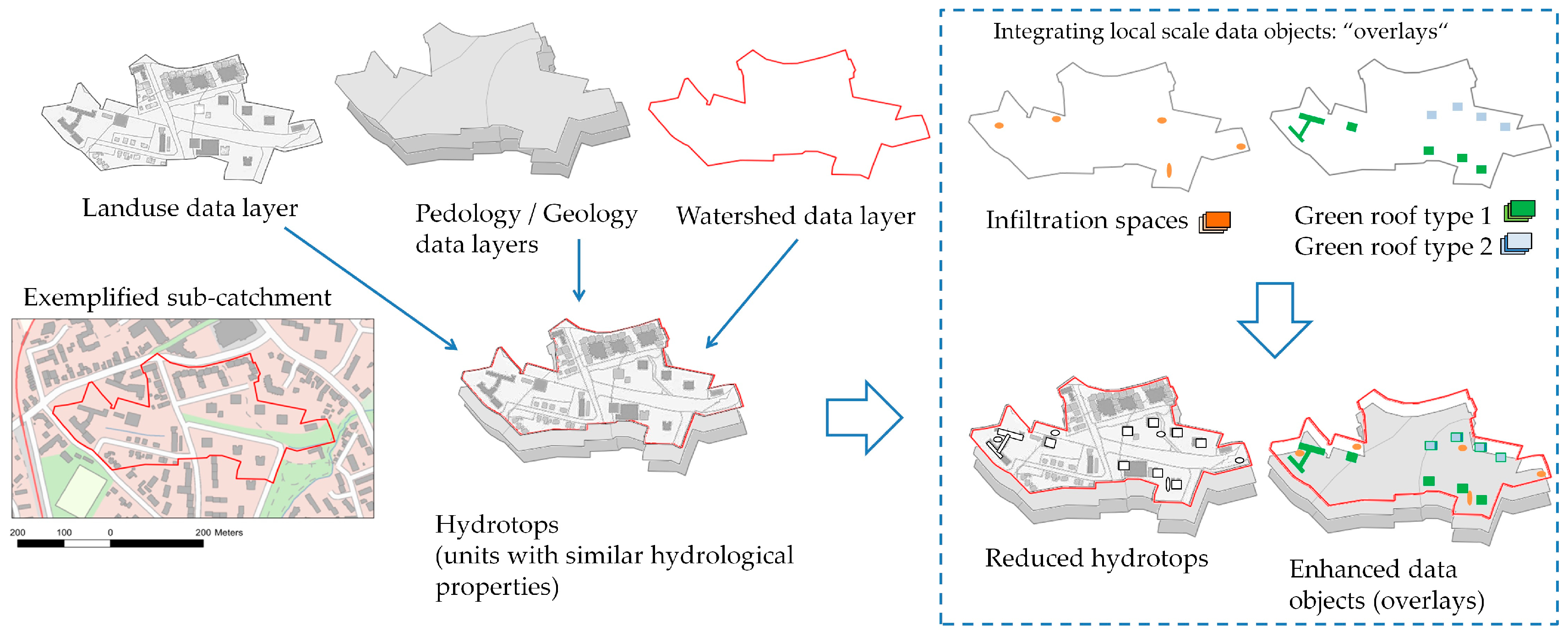
Figure 3.
Enhancement of a network structure to integrate multiple linked data objects.

Figure 4.
Data objects defined on respective spatial scales and new developed interconnections: (i) meso via reach scale; (ii) on reach scale; and (iii) on micro scale.
Figure 4.
Data objects defined on respective spatial scales and new developed interconnections: (i) meso via reach scale; (ii) on reach scale; and (iii) on micro scale.

Figure 5.
Computation procedure over the spatial and temporal scales.
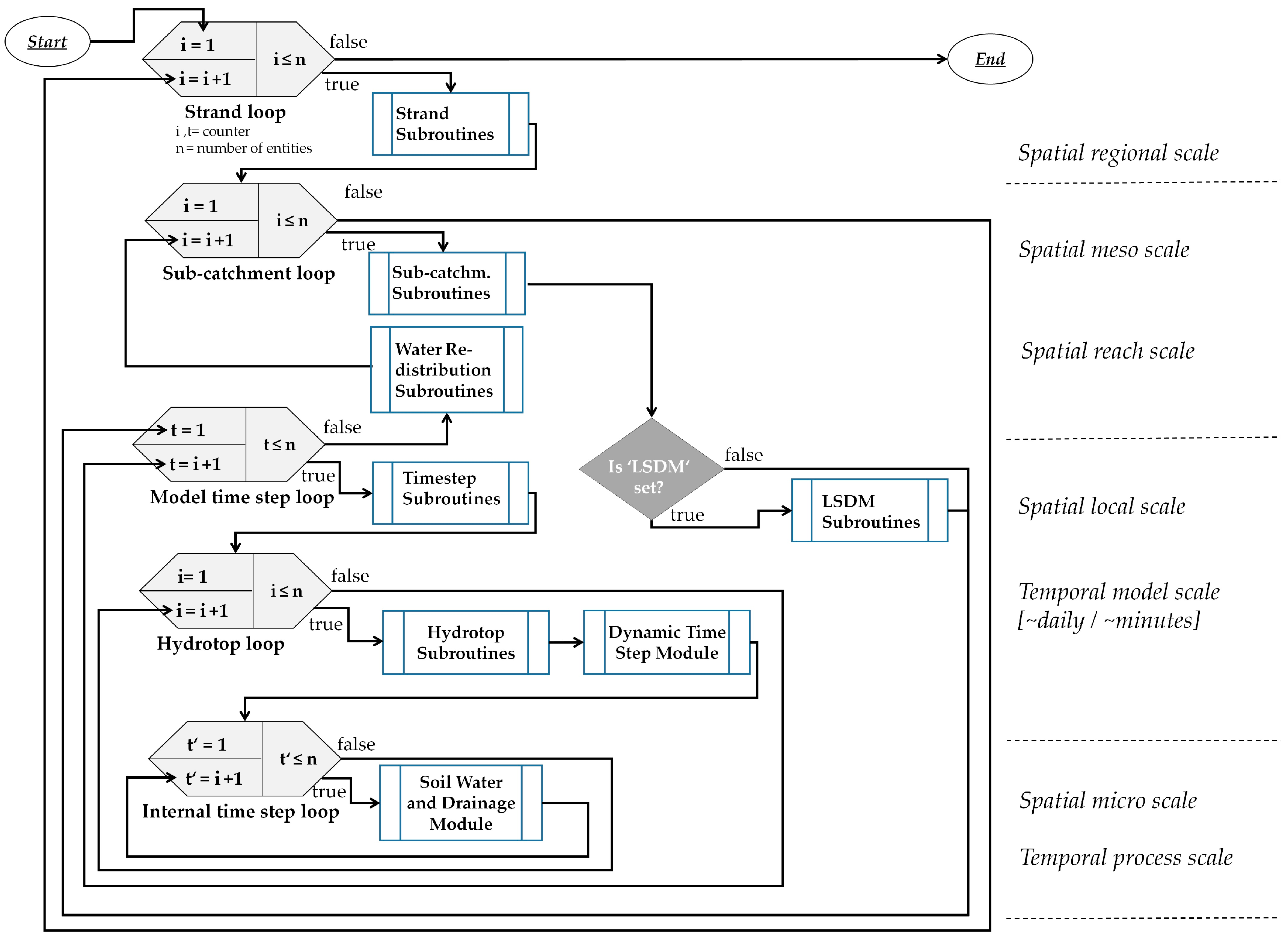
Figure 6.
Dynamic Time Step Size Module.

Figure 7.
Soil water and drainage module: Water balance computation procedure via four layer stages on the spatial and temporal micro scale with new developed drainage functions.
Figure 7.
Soil water and drainage module: Water balance computation procedure via four layer stages on the spatial and temporal micro scale with new developed drainage functions.

Figure 8.
Design examples of LSDM made up of multiple layers (L = layer): (a) green roof with overflow and down pipe outlet; (b) swale-filter-drain system with coupled layers; (c) swale; (d) cistern with rainwater harvesting function.
Figure 8.
Design examples of LSDM made up of multiple layers (L = layer): (a) green roof with overflow and down pipe outlet; (b) swale-filter-drain system with coupled layers; (c) swale; (d) cistern with rainwater harvesting function.

Figure 9.
Laboratory physical model setup with the Rainfall-Simulator of the Hamburg University of Technology (RS-TUHH) and two green roof test installations.
Figure 9.
Laboratory physical model setup with the Rainfall-Simulator of the Hamburg University of Technology (RS-TUHH) and two green roof test installations.
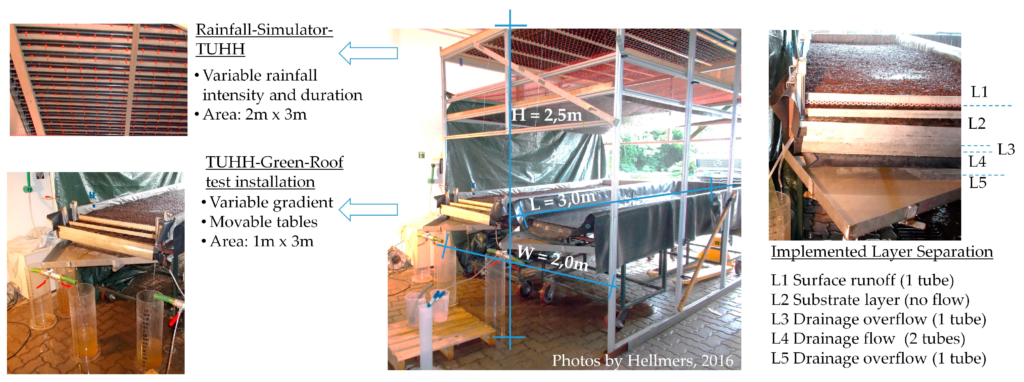
Figure 10.
Numerical model setup: Schematic design and input parameters.
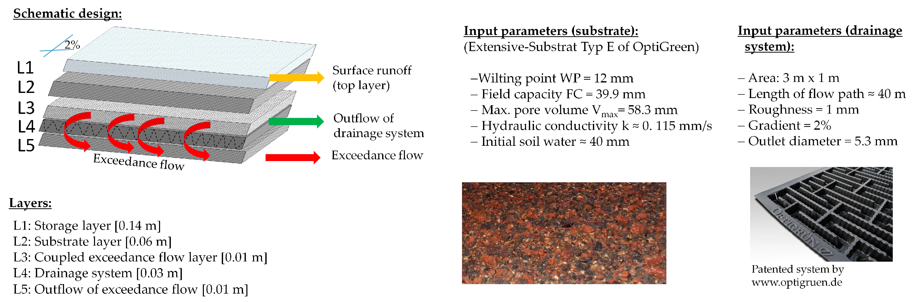
Figure 11.
Results of the calibration run: precipitation of 1.8 mm/min for a duration of 15 min. Comparison between observed and simulated flux of the layered green roof model in hydrographs (left side) and scatter plots (right side).
Figure 11.
Results of the calibration run: precipitation of 1.8 mm/min for a duration of 15 min. Comparison between observed and simulated flux of the layered green roof model in hydrographs (left side) and scatter plots (right side).
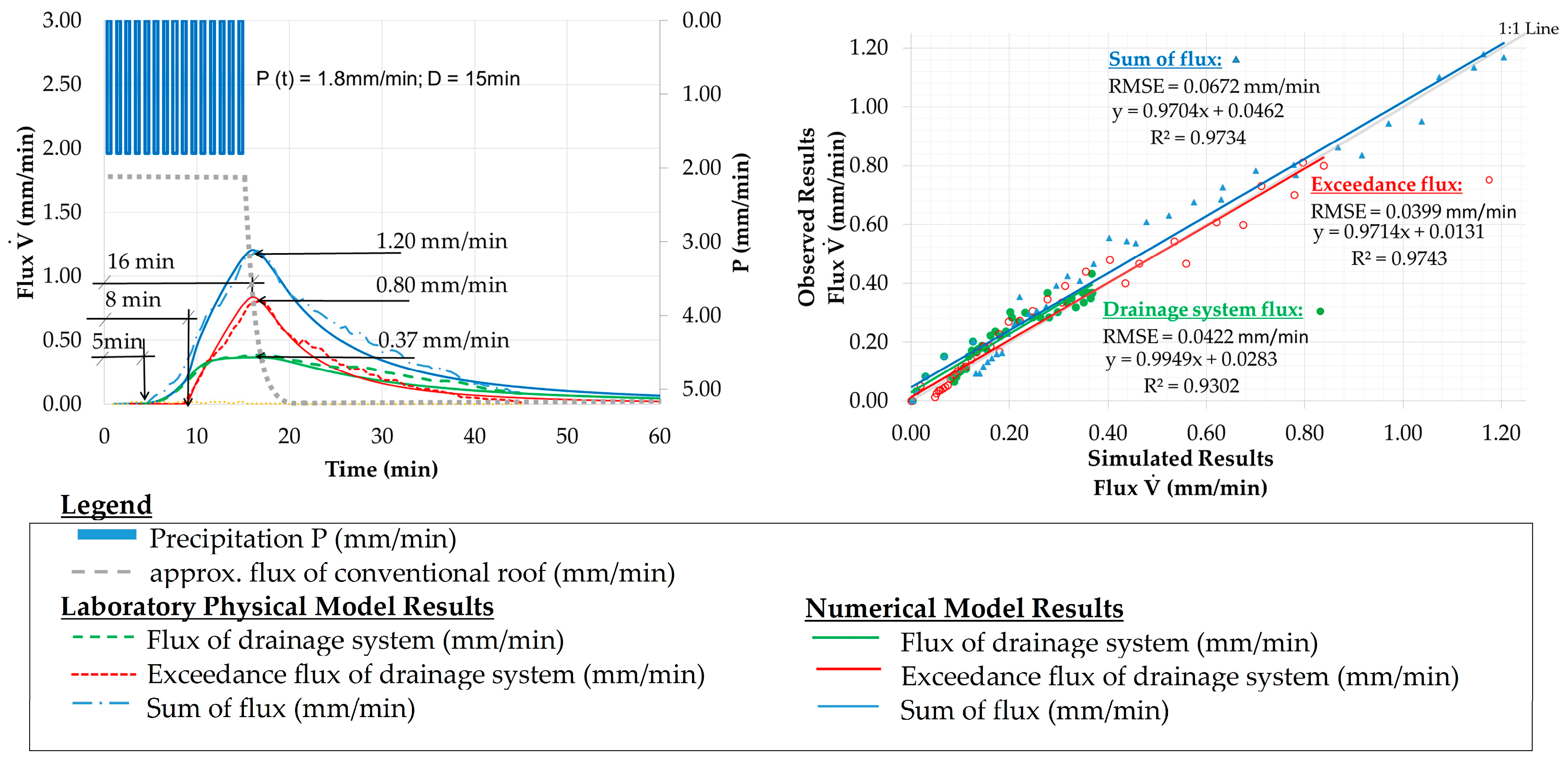
Figure 12.
Results of the validation run 1: precipitation intensity P(t) of 1.0 mm/min for a duration of 45 min. Comparison between observed and simulated flux of the layered green roof model.
Figure 12.
Results of the validation run 1: precipitation intensity P(t) of 1.0 mm/min for a duration of 45 min. Comparison between observed and simulated flux of the layered green roof model.

Figure 13.
Results of the validation run 2: precipitation intensity P(t) of 0.6 mm/min for a duration of 90 min. Comparison between observed and simulated flux of the layered green roof model.
Figure 13.
Results of the validation run 2: precipitation intensity P(t) of 0.6 mm/min for a duration of 90 min. Comparison between observed and simulated flux of the layered green roof model.


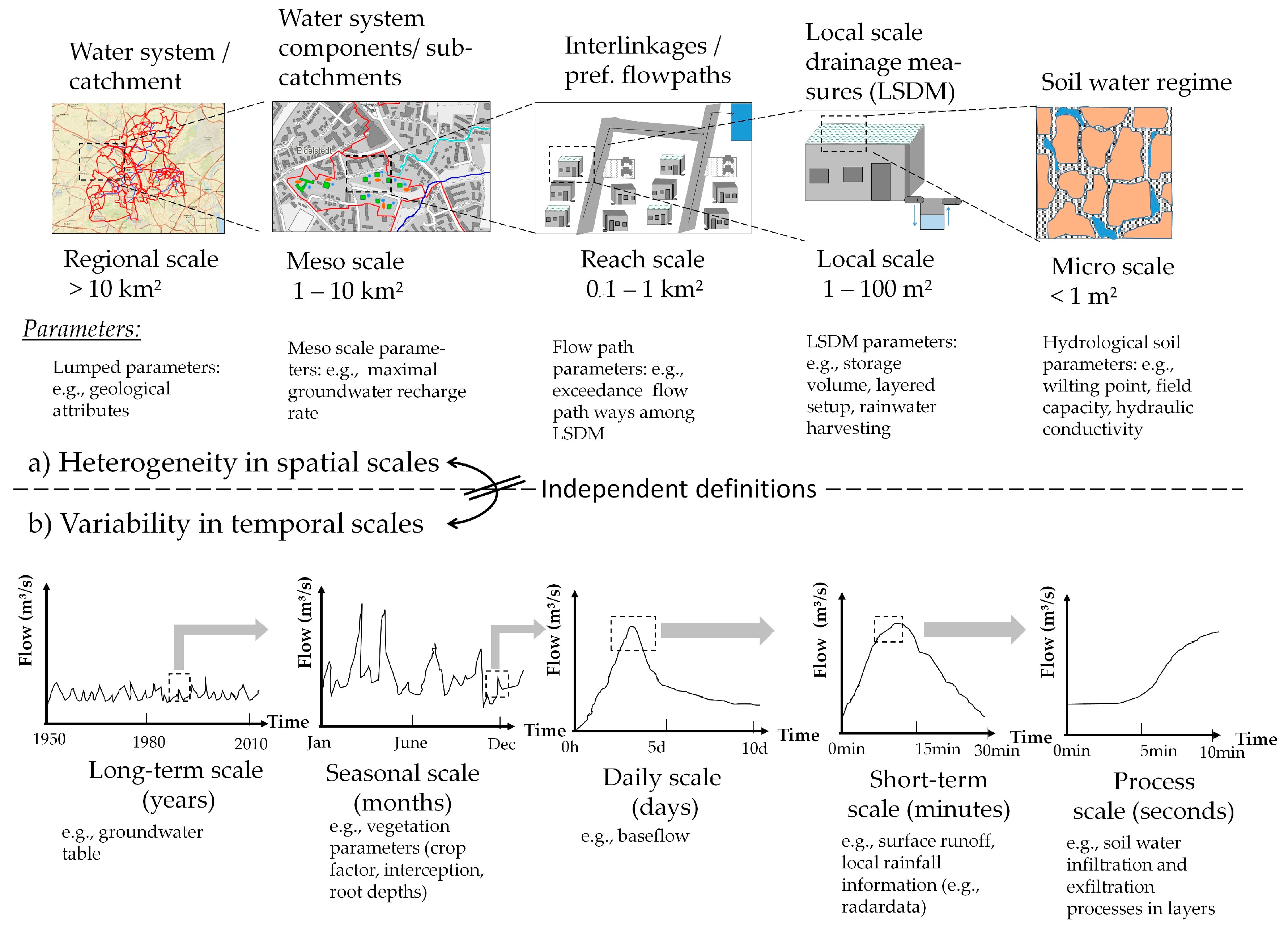
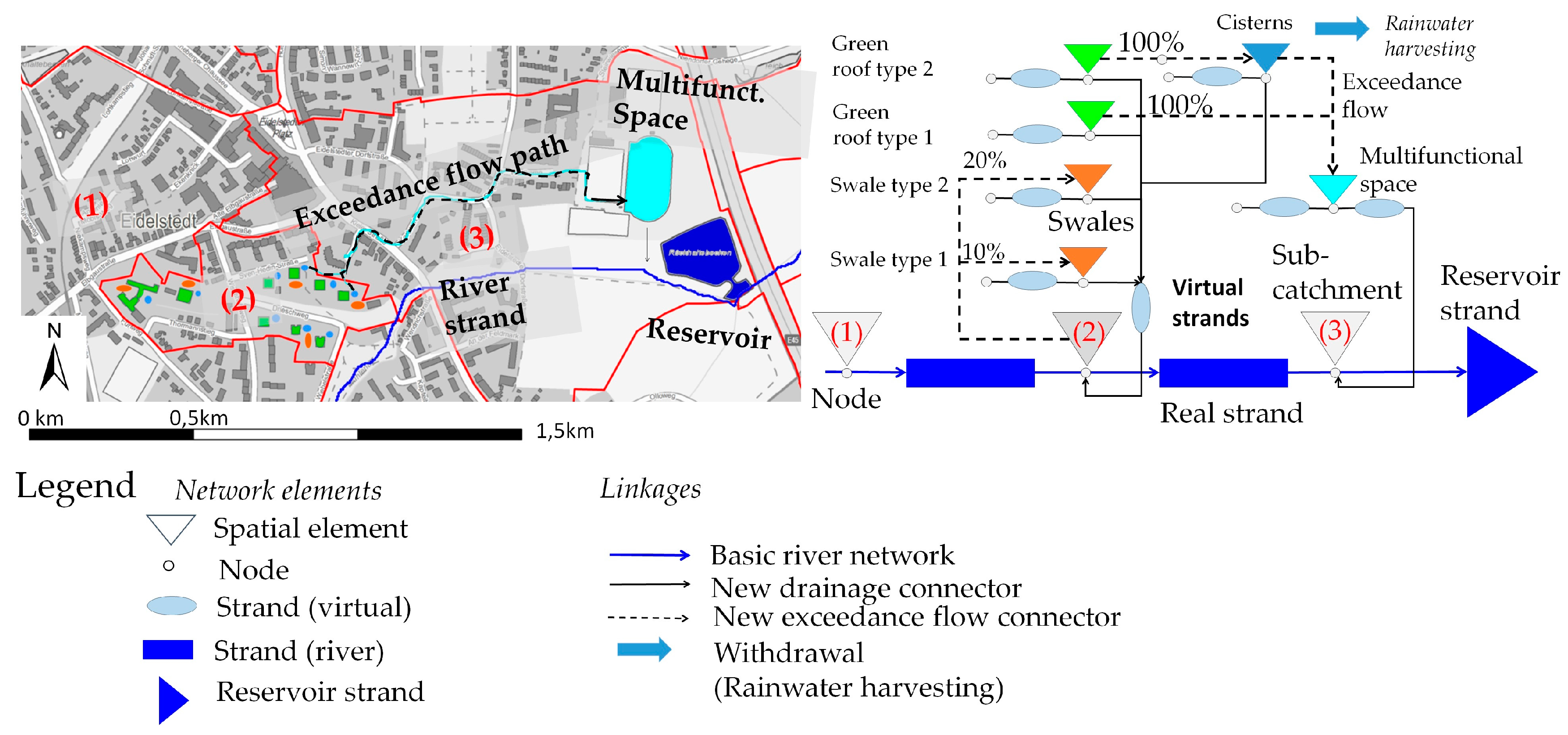
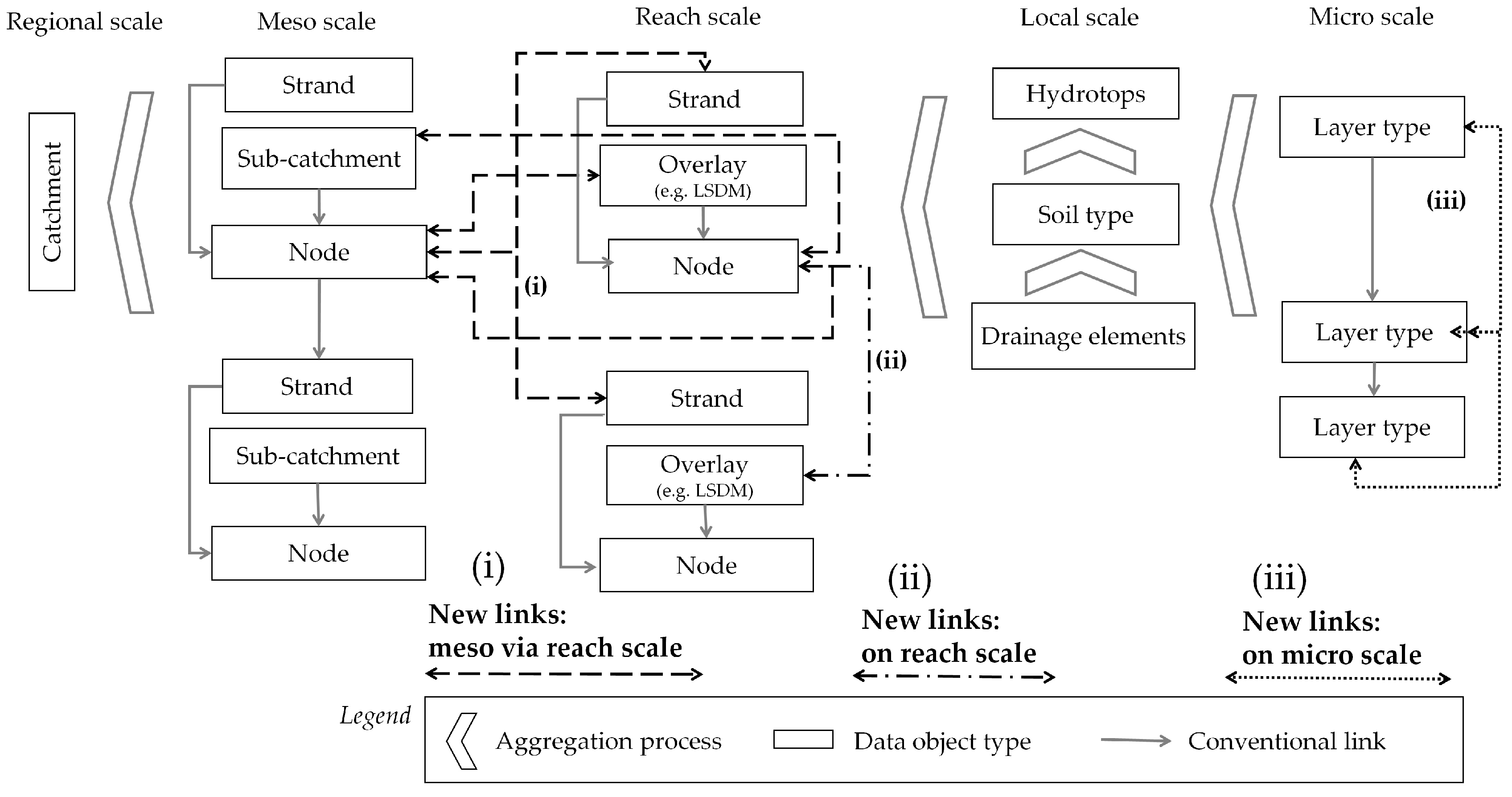
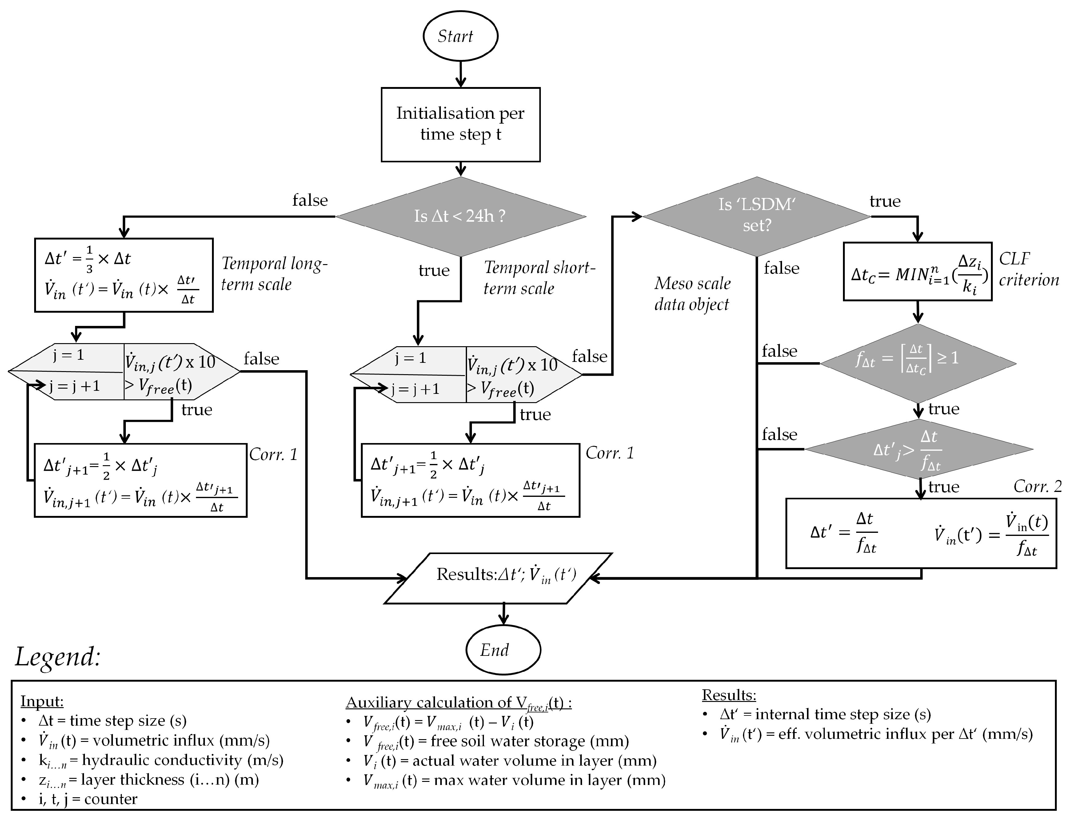
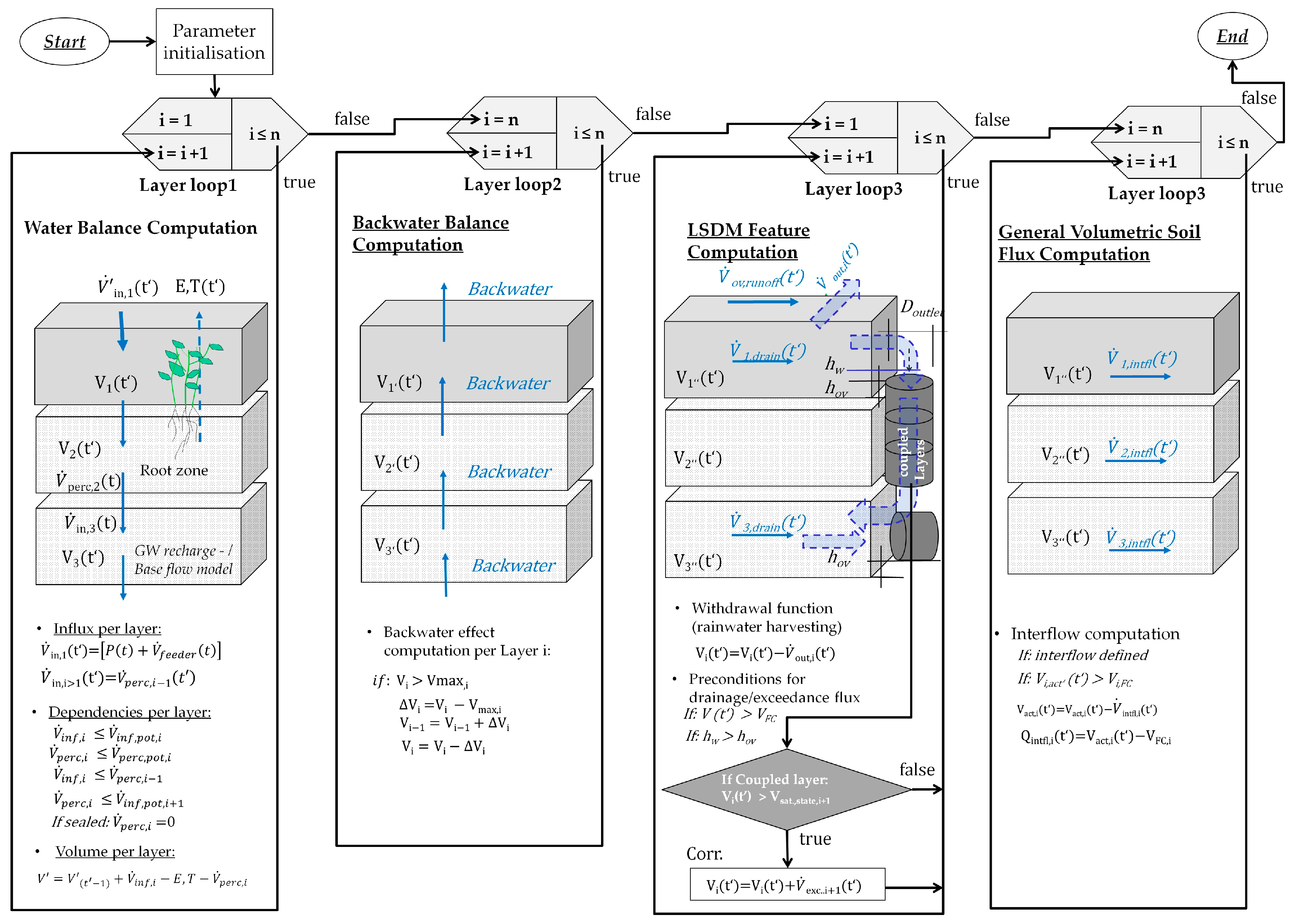
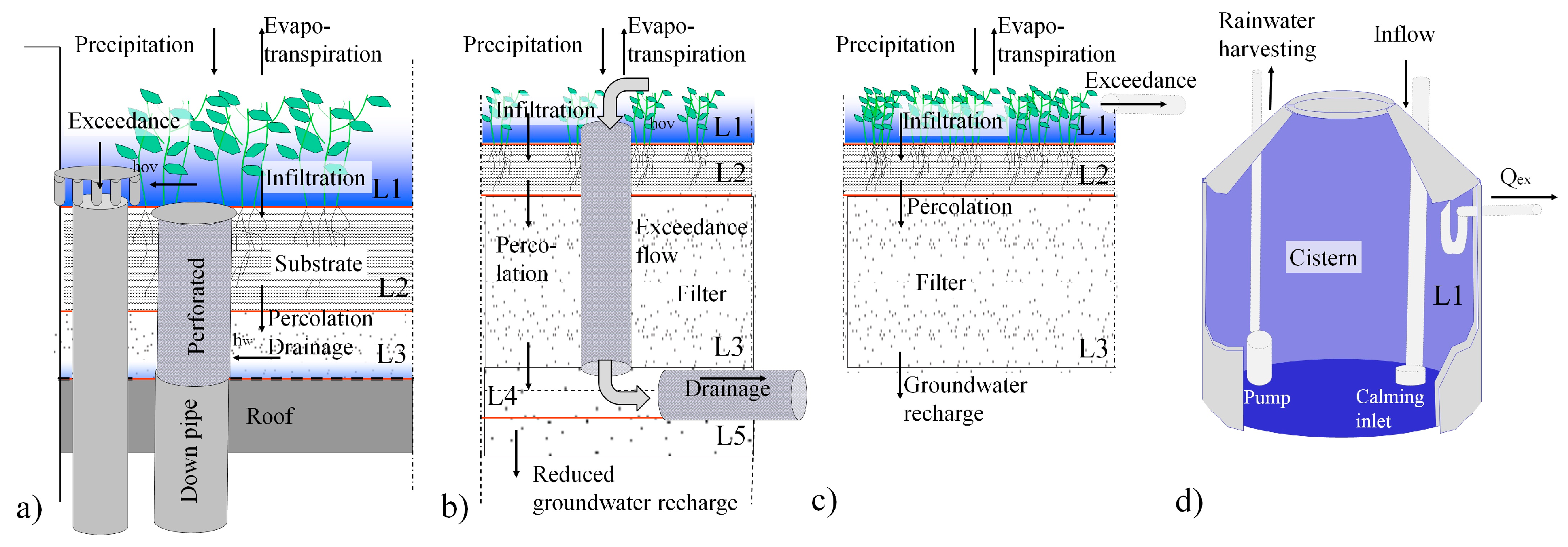
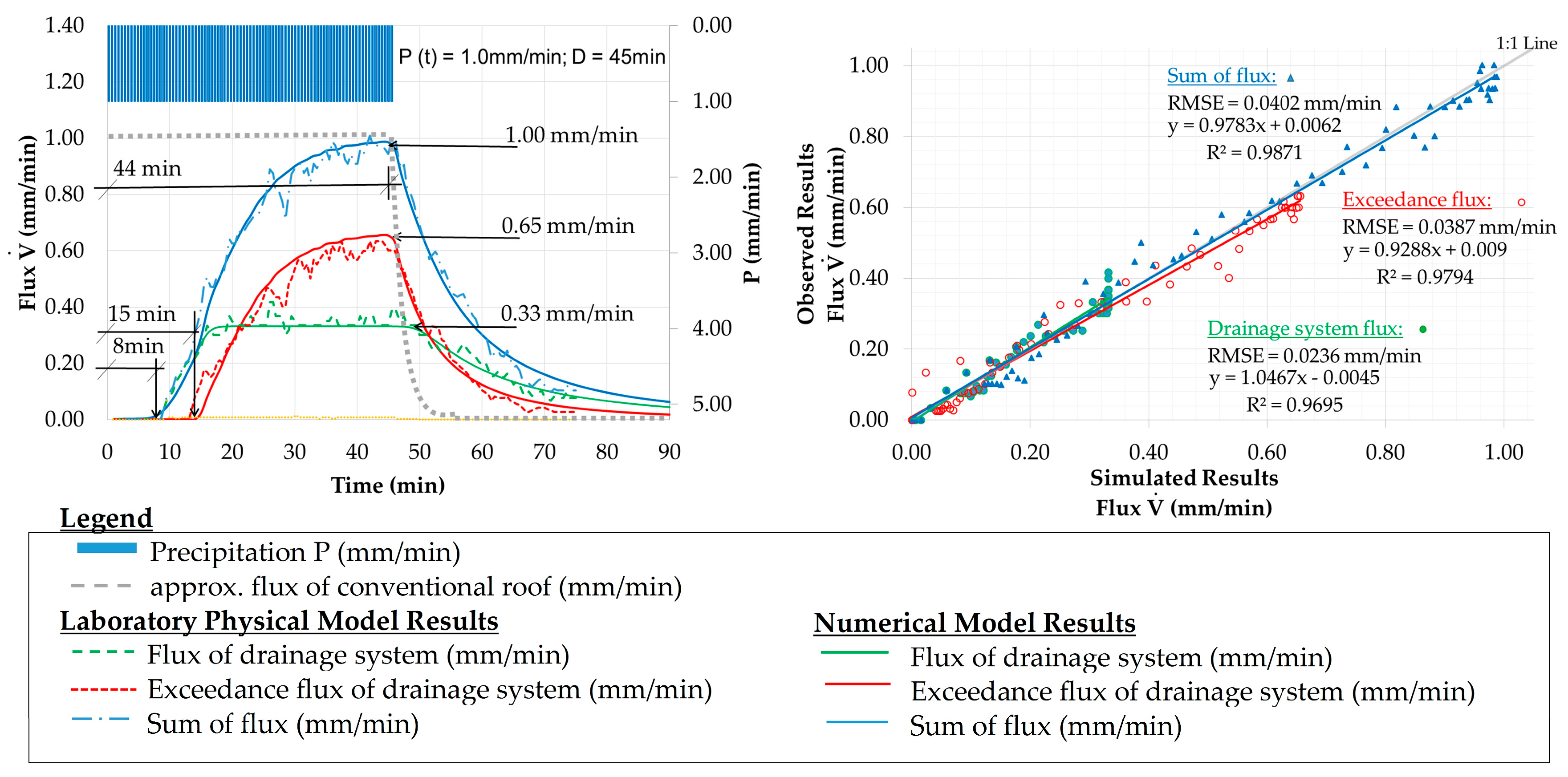
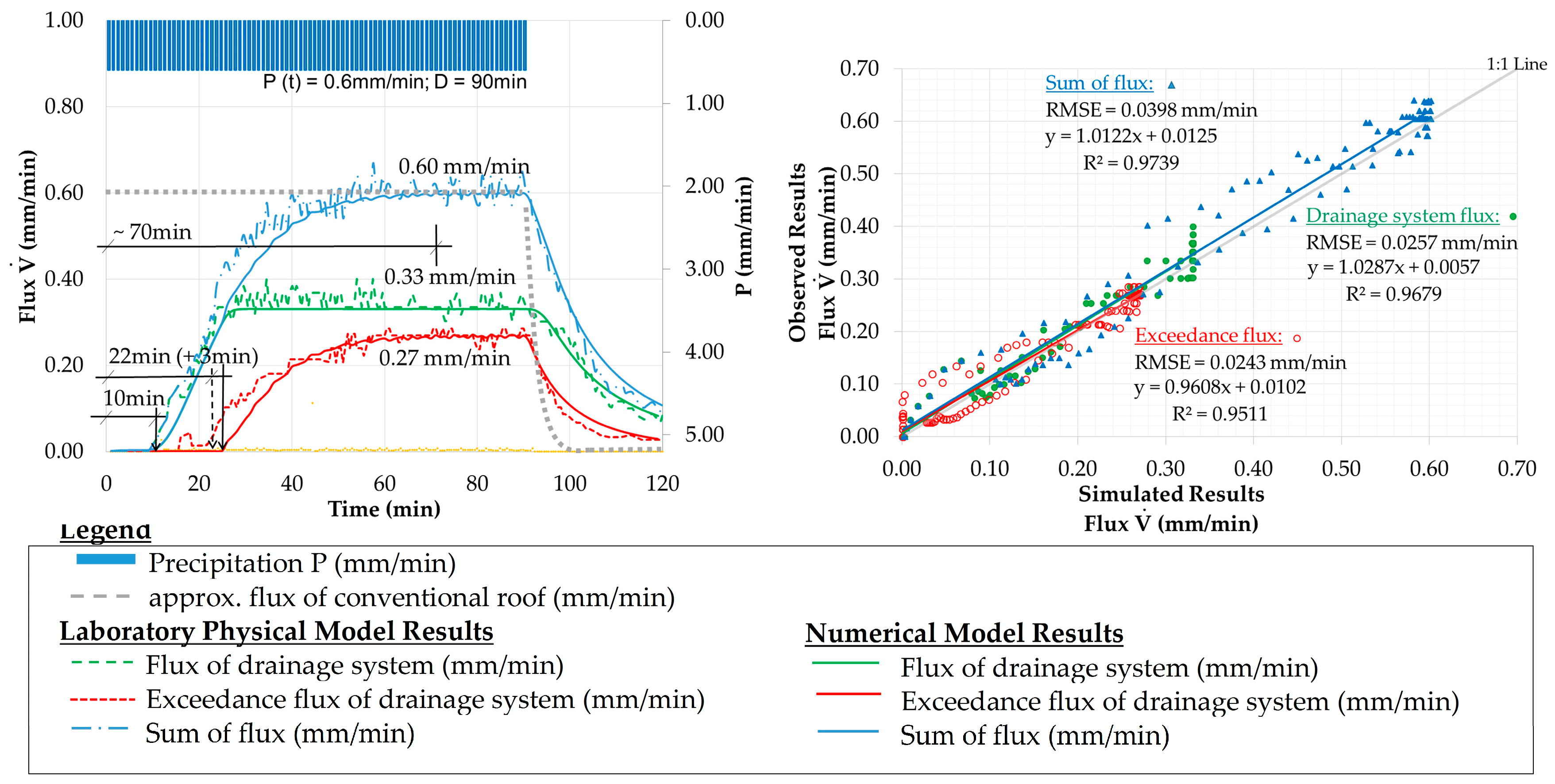
| Cali- and Validation Runs 1 | Drainage System Criteria | Exceedance System Criteria | ||||||||
|---|---|---|---|---|---|---|---|---|---|---|
| (1) | (2) | (3) | (4) | (5) | (1) | (2) | (3) | (4) | (5) | |
| Δ in Time Delay (min) | Δ in Time to Peak Flux (min) | Δ in Peak Flux (%) | Δ in Volume (%) | RMSE (mm/min) | Δ in Time Delay (min) | Δ in Time to Peak Flux (min) | Δ in Peak Flux (%) | Δ in Volume (%) | RMSE (mm/min) | |
| Cal. 1 | <1 min | <1 min | 7.5% | <10% | 0.0422 | <1 min | <1 min | 4.5% | <10% | 0.0399 |
| Val. 1 | <1 min | <1 min | 10.0% | <10% | 0.0236 | <1 min | <1 min | 3.0% | <10% | 0.0387 |
| Val. 2 | <1 min | <1 min | 3.5% | <10% | 0.0257 | ~3 min | <1 min | 10.0% | <10% | 0.0243 |
Notes: 1 Calibration Run 1: P(t) = 1.8 mm/min, D = 15 min; Validation Run 1: P(t) = 1.0 mm/min, D = 45 min; Validation Run 2: P(t) = 0.6 mm/min, D = 90 min.
© 2017 by the authors. Licensee MDPI, Basel, Switzerland. This article is an open access article distributed under the terms and conditions of the Creative Commons Attribution (CC BY) license ( http://creativecommons.org/licenses/by/4.0/).
Share and Cite
MDPI and ACS Style
Hellmers, S.; Fröhle, P. Integrating Local Scale Drainage Measures in Meso Scale Catchment Modelling. Water 2017, 9, 71. https://doi.org/10.3390/w9020071
AMA Style
Hellmers S, Fröhle P. Integrating Local Scale Drainage Measures in Meso Scale Catchment Modelling. Water. 2017; 9(2):71. https://doi.org/10.3390/w9020071
Chicago/Turabian StyleHellmers, Sandra, and Peter Fröhle. 2017. "Integrating Local Scale Drainage Measures in Meso Scale Catchment Modelling" Water 9, no. 2: 71. https://doi.org/10.3390/w9020071
Note that from the first issue of 2016, this journal uses article numbers instead of page numbers. See further details here.