1. Introduction
In the last decades, there has been widespread implementation of Green Infrastructures (GIs) worldwide [
1,
2]. GIs retain, treat and reduce stormwater, contributing to runoff management, flood mitigation, landslide prevention, air quality management, and further mitigate the warming effects related to climate change and urban heat islands. In highly urbanized catchments, the use of GIs is limited by the available soil surface area. Green roofs (GRs), within the much wider context of GI, could represent a flexible solution to this problem [
3]. Built at relative low costs on rooftops, extensive GRs remove a large fraction of impervious surfaces from the urban hydrological cycle, thereby providing the mentioned benefits [
4,
5,
6,
7,
8,
9].
The stormwater response of a green roof is highly impacted by the green roof structure itself and, to a larger extent, by the climate conditions, making generalization of the GR hydrological performance a very difficult task [
10]. Various scientific contributions, proposed in the recent past, comment indeed on an extremely variable level of rainwater reduction. Green roofs appear to reduce total yearly runoff volume by 40% to 90%, with an important seasonal fluctuation. The peak flow rate can be even more attenuated, i.e., by 20% to 90% [
11,
12,
13,
14]. The GR hydrological behaviour is modelled by soil water balance approaches. Conceptual or more physically based, oriented to the event or to the continuous time scale, suitable for single building or catchment scale, a broad range of models have been proposed by numerous authors [
15,
16,
17,
18,
19,
20]. Their implementation generally requires a high number of input parameters related to the soil hydraulic properties including textural class of the soil, residual soil water content, saturated soil water content, saturated hydraulic conductivity, or related to the water flow boundary condition, and the initial condition in terms of the pressure head or the water content [
13,
21]. Additional complexity is related to one of the main processes to be modelled in a GR soil water balance, the evapotranspiration loss. Evapotranspiration continuously restores the retention capacity of a storage system, because it directly acts on its moisture content, and thus on its ability to retain water after rainfall events. Actual evapotranspiration is generally evaluated starting with the potential rate, weighted by a coefficient computed in different ways, e.g., the ratio of actual moisture content to the field capacity of the substrate [
17], a function of the hygroscopic saturation, the average saturation over the root zone and the soil water content at stomatal closure [
16]. Model implementation to predict the effectiveness of a planned green-roof installation in a particular area is mostly complex, due to the above-mentioned required data and parameters of the hydraulic system to be simulated, which are usually not readily available without laboratory or field experiments.
The objective of this paper is twofold. Firstly, a conceptual model approach is proposed as an answer to mentioned modelling limitations, as it essentially requires only few basic input parameters and weather data recorded by inexpensive monitoring installations in the area of interest. Although simple, the GR runoff production is simulated by a surface balance between input and output meteorological fluxes, that are rainfall and actual evapotranspiration (AET). No calibration is needed. The actual evapotranspiration loss process is considered as a climate forcing variable, in the same way as precipitation, for which an a-priori assessment can be provided. Secondly, the efficiency of empirical relationships for AET estimation is tested. Actual evapotranspiration fluxes are strongly driven by water availability (water availability limited systems) on one hand and soil water abstraction atmosphere power (energy limited systems) on the other. For each approach, an empirical model had been applied and their quality evaluated through comparison between observed and modelled runoff.
2. Materials and Methods
2.1. The Experimental Data
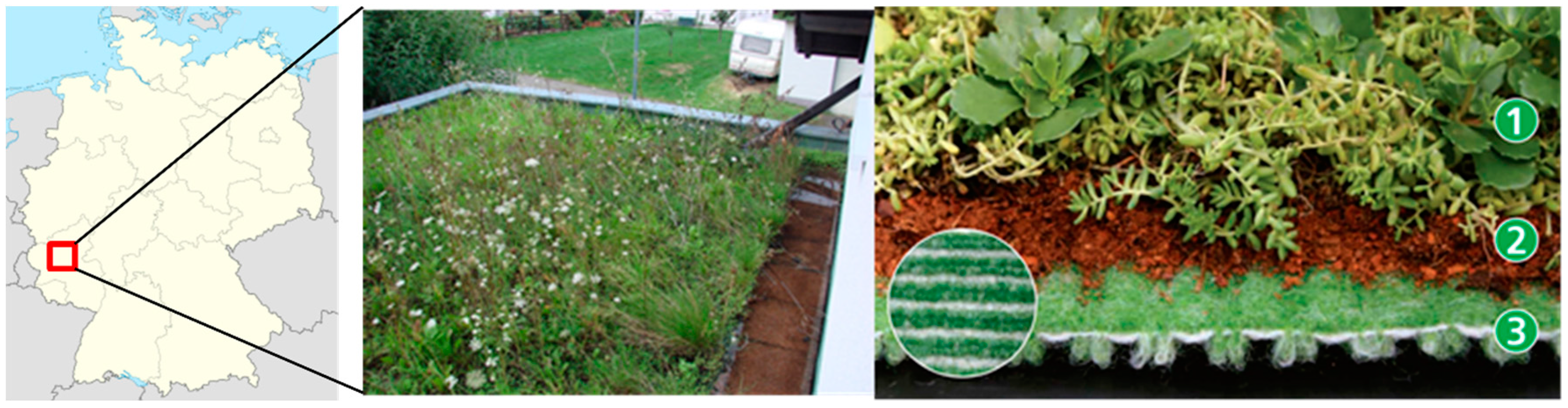
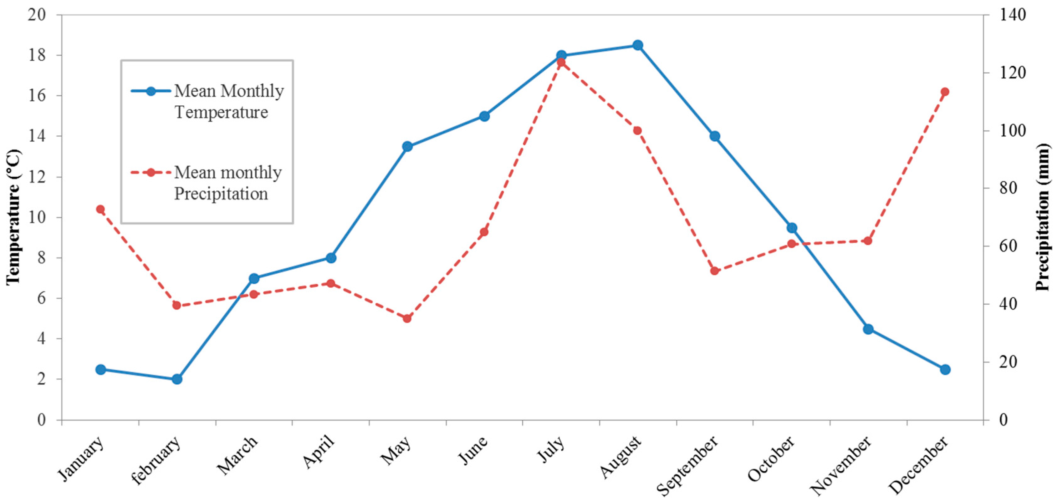
The studied green roof is located near Bernkastel-Kues, Rhineland-Palatinate, Germany (
Figure 1) at Longitude 7.075903415679932, Latitude 49.9197855721214 and Altitude 145 m with typically oceanic climate, featured by warm summers and cool winters. Average precipitation is about 700–800 mm/year and it is approximately uniformly distributed during the year. Temperature exhibits instead a typical seasonal pattern, with highest monthly mean values during the summer season of about 18 °C (
Figure 2).
Meteorological data such as wind speed, air temperature, relative humidity, global radiation and atmospheric pressure have been collected at the nearest available meteorological station, Bernkastel [
22], whereas precipitation has been recorded at the GR site. The roof is of extensive type, it has a surface of 22 m
2, a depth of approximately 15 cm and a slope less than 5°. It is composed of three layers: the vegetation layer, the growing medium and a water storage/protective layer (
Figure 1). The vegetation layer is made of sedum and spontaneous vegetation, the growing medium is a mineral substrate and the water storage/protective layer is a retention Hydrotex membrane. Runoff measurements have been recorded, with a daily time step, from March 2004 to May 2007, but some missing data appear during the monitoring period, preventing the total period of observation to be used for modelling purposes. Additionally, no significant runoff has occurred, due to freezing of the water, between late December and late March. For this reason, the winter period has not been considered in the simulation approach.
2.2. The Conceptual Model
The approach used in this paper to quantify GR runoff production is based on a water balance conceptual model, consistent with the saturation excess runoff process, as the dominant mechanism [
23]. When rainfall reaches the green roof surface, it is partially intercepted by the vegetation and partly infiltrates into the substrate and storage layer, where it is retained. Rainfall volume exceeding the storage capacity is routed downstream. During non-rainy periods, evapotranspiration restores the water retention capacity. The daily scale governing equations for the production of runoff are:
where “
t” is the daily time index, V is depth of water in the green roof, P the total observed precipitation, AET the actual evapotranspiration, R the runoff and W
max is the maximum water holding depth. In order to develop a tool for green roof planning simply based on climate variables, the proposed model is marked by some simplifications. As will be shown later in the
Appendix A section, it is possible to assume that the maximum water holding depth on day “
t” is related to the water depth on day “
t − 1” as follows:
Thus, the runoff production Equation (1) can be rewritten as:
The runoff production can then be modelled at daily time steps as the result of a surface water balance between input and output fluxes. AET is simulated with the use of indirect methods (empirical relationships) and thus the choice of the particular AET approach would be crucial for model uncertainty. To further consider the ability of the evapotranspiration process to restore the green roof water retention capacity during prolonged dry periods [
17], a cumulative soil water balance index over the previous four days is considered:
If the index produces a negative value on the day “t”, the GR retention capacity is assumed to be completely restored. No runoff will be produced on that day, if its actual rainfall does not exceed the GR retention capacity. The four-day interval in Equation (4) has been calibrated on the basis of available monitoring data about dry periods, which represent a negligible set of occurrences (about 3% of total cases), perhaps due to the particular uniform precipitation regime of the studied area. Equation (4) has been applied regardless of the relationship used for actual evapotranspiration modelling.
The simplified proposed approach for daily scale GR hydrological production described by Equation (3) does not require an explicit calibration process as predicted GR response to rainfall is computed as the difference between observed precipitation and modelled actual evapotranspiration. However, the model requires an initial value for the depth of water V, which is assumed to correspond to the Antecedent Precipitation Index value, considered as a proxy of soil moisture conditions. (API [
24]). The same index would be used, as later illustrated, to compute AET losses.
2.3. Modelling A-Priori Actual Evapotranspiration (AET)
In contrast to most common frameworks, in the proposed approach evapotranspiration losses are modelled a-priori, as a function of meteorological parameters, independently of explicit moisture content. Actual evapotranspiration fluxes are strongly driven by water availability (water availability limited systems) on one hand and soil water abstraction atmosphere power (energy limited systems) on the other. The proportion by which the two factors contribute to the evapotranspiration and probably also the period of the year, when one factor prevails over the other, are linked to the average climate regime of the area under examination [
25]. Following this concept, a water availability limited and an energy limited scheme have been investigated. Those are the API model [
24] and the Advection-Aridity (AA) model [
26] respectively, both belonging to the category of models based on complementary relationship (CR) [
17]. Considered AET models require previous calculation of Priestley-Taylor [
27] PET potential evapotranspiration flux:
where
is the slope of the saturation vapor pressure–temperature curve (kPa·°C
−1), given by the formula:
and T
mean is the average temperature between maximum and minimum values during the day (°C), γ is the psychrometric constant (kPa·°C
−1), λ is latent heat of vaporization (MJ·kg
−1), Rn is the net radiation (MJ·m
−2·day
−1), G is the soil heat-flux density at the soil surface (MJ·m
−2·day
−1), considered to be negligible on a daily time scale [
28].
The API model [
24,
29] predicts AET rates modifying the PET Priestley-Taylor equation through a coefficient “α” related to the antecedent precipitation index API [
30]:
where the dimensionless coefficient, α, is expressed as:
assuming that for over saturated systems (API > 20 mm) AET rates are no longer dependent on soil water content but they are a constant percentage of PET [
29]. The Advection-Aridity model [
27] calculates AET from PET predicted by coupled Priestley-Taylor and Penman equations, according to the formula [
29]:
where:
u
2 is the wind speed (ms
−1), e
s is the saturation vapor pressure (kPa), and e
a is the vapor pressure (kPa), Δ, γ, R
n and G previously described and α is the advection correction coefficient from the Priestley-Taylor model equation. In the following a-priori AET assessment approach, focus has been given to the uncertainty in the chosen AET formulation that would propagate through the modelled system.
3. Results
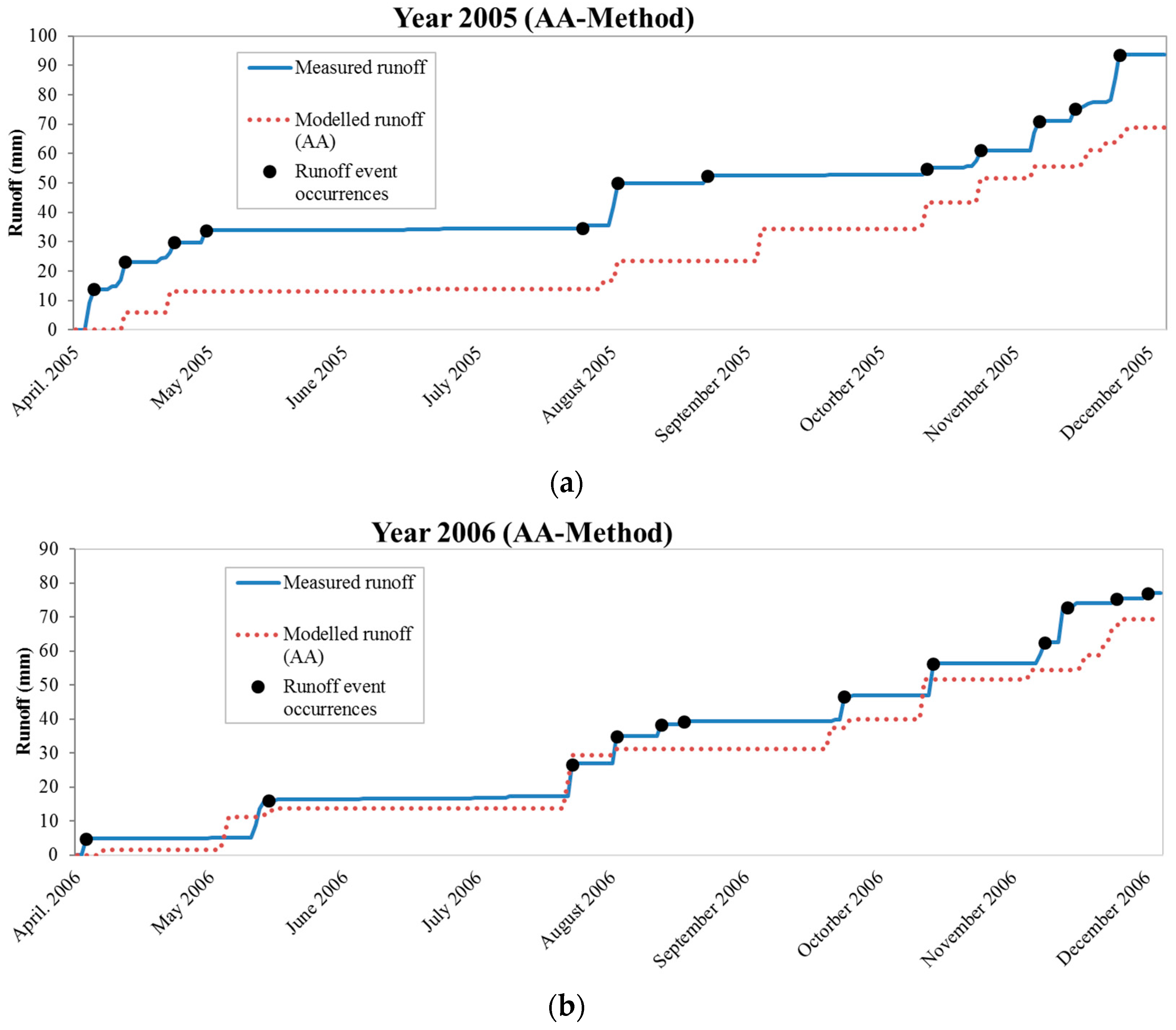
Provided data continuity and reliability, the period chosen for the simulations ranges from April 2005 to December 2006. In the following, seasonal scale and event scale analyses have been performed. The seasonal scale analysis refers to three different periods: spring from April to June, summer from July to September and autumn from September to December. As previously mentioned, the winter season has not been considered in the current analysis.
3.1. AET Assessment
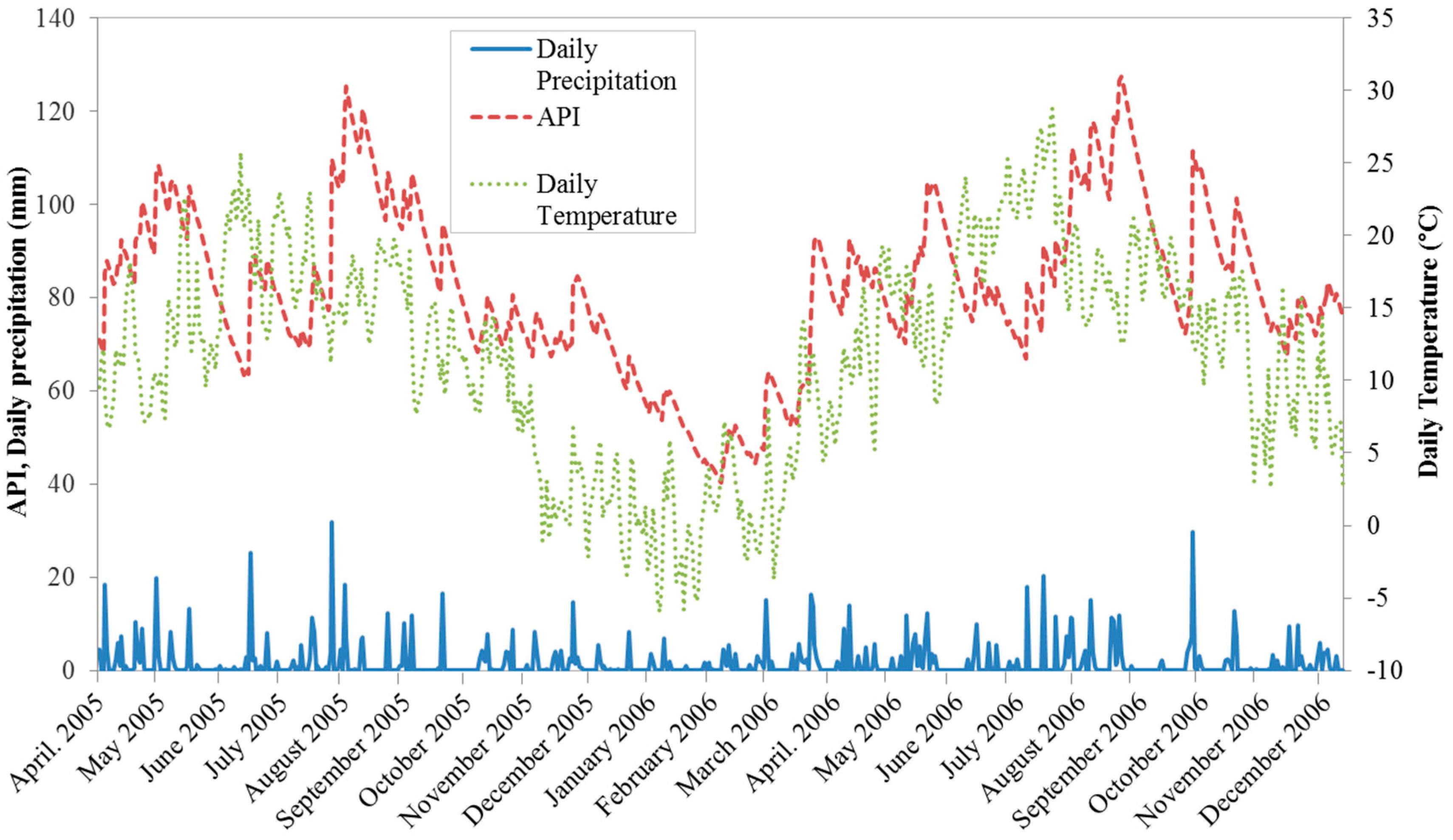
As previously introduced, the API model and the Advection-Aridity model for a-priori assessment of actual evapotranspiration have been applied here. These are considered respectively as the two main controls on actual evapotranspiration fluxes, which are the water availability, described by the API index, and the soil water abstraction atmospheric power. Main meteorological variables used for AET assessment are illustrated in
Figure 3.
Along with daily observation data, the API index is also plotted [
30]. The API represents the antecedent moisture content prior to a rainfall event, computed as a weighted summation of daily precipitation depths as follows
where API
t is the antecedent precipitation index computed on day
t, C the storm hydrograph recession coefficient and P
t the precipitation of day
t. AET estimations have been reported in
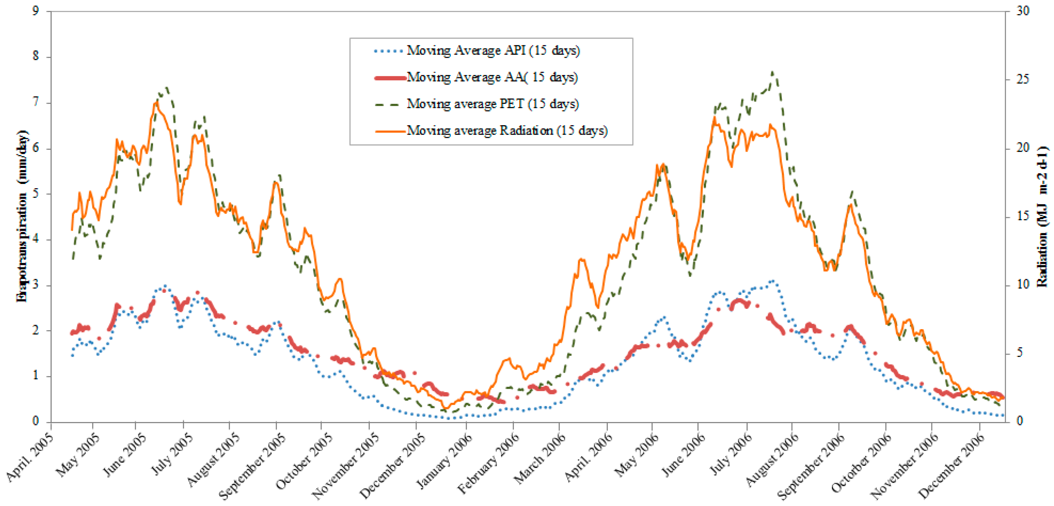
Table 1 and also as monthly patterns in
Figure 4 for the full period of observation. Regardless of the methods, the AET is featured by a sinusoidal pattern, with the maximum and minimum values occurring during the summer and autumn period, respectively (
Figure 4).
The AA method systematically predicts large AET amounts compared to the API model during the year 2005. For the total annual amounts, the difference is about 20% with a maximum value of about 76% for the autumn period during the year 2005 (
Table 1). During the year 2006, the relative relation between the AA and the API method changes, in that the AA method predicts smaller AET amounts, comparable to the API method predictions (the difference is about 2% over the total period), with the exception of the autumn season, where AET
AA overestimates AET
API of about 40%.
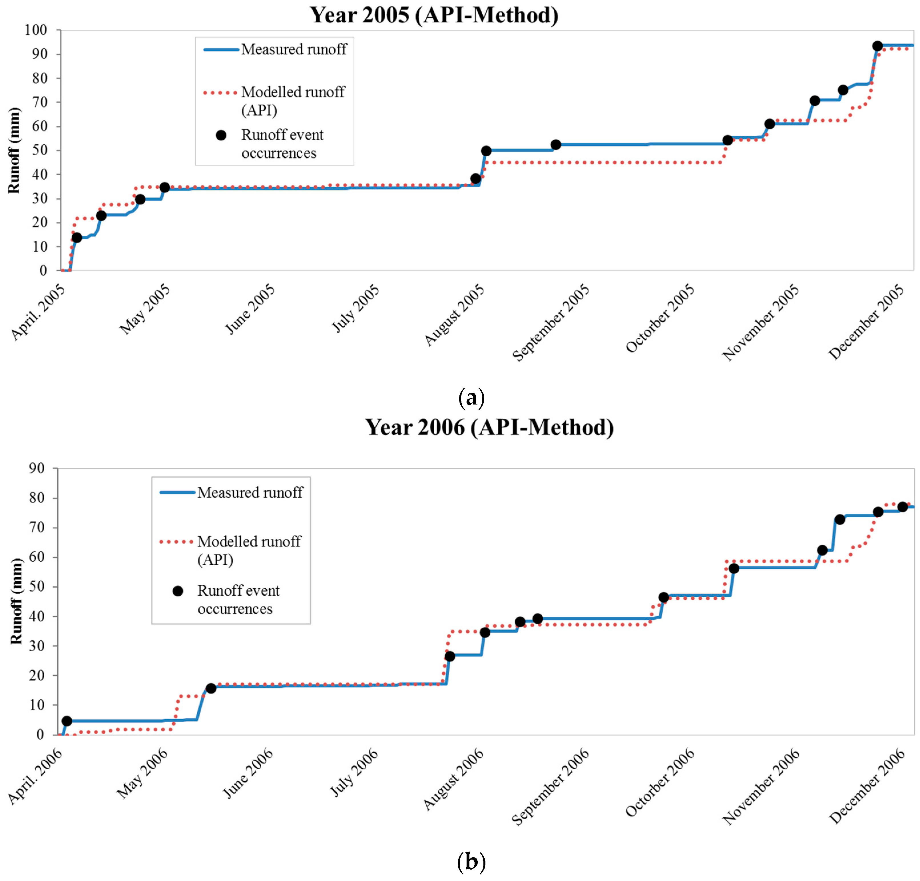
3.2. The GR Model Performances
Equation (3) has been applied to compute runoff for the observed period. In order to quantitatively measure the ability of the model to fit the available data, three goodness-of-fit (GOF) indices are calculated. These indices summarize the discrepancy between the cumulated measured runoff and the cumulated simulated values obtained by the conceptual water balance. The indices are the root-mean-square errors (RMSEs), the averages of absolute percentage errors (AAPEs), the relative percentage errors (RPEs), estimated as follows:
where “
n” is the number of points of discontinuity of the cumulated runoff distribution (occurrences of runoff events) where the fit is valuated, R
mod is the modelled runoff and R
obs the observed runoff. RMSE and AAPE are used for the seasonal scale assessment whilst RPEs is used for the event scale assessment (
Figure 5 and
Figure 6).
Regarding the analysis on a seasonal basis, the indices RMSE and AAPE have been compared to the total amount of runoff during the considered period. In particular for the API model, AAPE indices for the total period show moderate average errors ranging between 8% in 2005 (
Table 2) and 12% in 2006 (
Table 3).
Good performances are predicted also on the seasonal base, where underestimation generally occurs during the summer period (10%–12%), and overestimation occurs during the remaining period (2%–17%). Seasonal summer underestimation probably occurs in response to enhanced modelled AET losses (without calibration) caused by large API values approached during this period (rainy period). Similarly, RMSE values indicate satisfactorily performances, ranging between about 1% and 3%, when compared to total observed runoff. The AA model shows instead higher errors than the API model. AAPE indices for the total period show average errors ranging between 118% in 2005 (
Table 2) and 19% in 2006 (
Table 3). Worst performances are predicted also on the seasonal base, where the tendency for over and underestimation in particular periods is no longer clear, AAPE ranges from 17% to 135% and RMSE, compared to total observed runoff, ranges from 1% to 14%.
Furthermore, an event scale analysis is performed, for which the RPEs is used as the goodness-of-fit measure.
Table 4 and
Table 5 show, that for the two years of simulation, for the API Model the absolute maximum value for RPEs is about 30%, while for the AA Method the runoff underestimations approach errors of about 300%.
In particular, according to the API model, runoff overestimation (max 36% on 20 April 2005) generally occurs during the warmer period of the simulation, i.e., the spring and summer seasons, whereas underestimation (max 24% on 24 November 2006) generally occurs in late summer and autumn seasons. In the case of the AA model, the hydrological scheme tends to consistently underestimate runoff during the total period, with errors ranging from 9% to 300%.
4. Discussion and Conclusions
A relative simple mono-dimensional approach is presented to predict the hydrological behavior of a green roof. The model is based on meteorological variables only. With some simplifications, it requires no parameter calibration. Through the use of empirical relationships, an a-priori assessment for actual evapotranspiration losses could be included, which proved the model to be an effective tool for green infrastructures efficiency planning.
However, the choice of that particular empirical relationship appeared to be crucial. If actual evapotranspiration losses are modelled with the use of a water availability limited scheme, errors appeared negligible (about 2%) and significant (about 40%) in the case an energy limited scheme is considered instead.
Environmental, climate and physical factors of the experimental site might have affected the simulation results. Applications to different case studies could further validate the potential of the proposed approach and, in particular, the better performances of the API model over the AA model. The water depth temporal pattern and the near coincidence between it and a dimensionless variable water holding capacity are discussed in the
Appendix A section. They lead to the conclusion that the most probable mechanism for runoff production is the saturation excess mechanisms and that actual evapotranspiration losses in those systems are dominated by soil water availability [
23].
The proposed framework has clearly some limitations that are discussed below. However, they are also the strength points of the proposal and make the approach suitable for planning sustainable urban drainage systems.
The first limitation is represented by the disconnection between the actual evapotranspiration losses and the soil moisture content, generally assumed as the hydrological model state variable, driving the rainfall-runoff transformation. Even though this represents a stretch on a physical processes base, comparisons between observed and modelled runoff indicate broad margins to consider the usefulness of empirical relationships into green infrastructure modelling, as commonly done in traditional catchment hydrology studies. In case of application to ungauged sites, one of the main objectives of the proposal, the choice of the empirical relationship would probably matter.
A second limitation is represented by the fact that, excluding the water depth stored into the green roof permeable layers from the water balance, does not enable the proposed model to explore the role of the particular green roof settings on green roof runoff control performances. Green roof constructions tend, however, to adapt to some commercial standards and the proposed scheme would still represent a valid methodology to be applied to the range of vegetated roof having similar characteristics.
Illustrated advantages and disadvantages outline a straightforward approach to investigate the effectiveness of planning variants for sustainable urban drainage systems to control runoff in urban areas. The model may also be used to predict the impact of climate conditions on such systems and also to explore their role in a future urban scale hydrological cycle, under potential climate variability scenarios.
Acknowledgments
The authors gratefully acknowledge funding provided through the Erasmus + program of the EU community that supported student mobility to Trier University of Applied Sciences. Authors thank all the anonymous reviewers and handling editor for their comments and help, which resulted in a significant improvement of the manuscript.
Author Contributions
All authors contributed to conceive and design the experiments; Joachim F. Sartor contributed to experimental data collection; Mirka Mobilia performed the experiments; all authors contributed to analyze the data, to write and revise the paper.
Conflicts of Interest
The authors declare no conflict of interest.
Appendix A. Analysis of the Wmax Capacity Variability
According to Equation (1), the GR runoff production is computed at the daily scale as:
Besides recorded P and modelled AET processes, to model runoff (R
mod), a value for the maximum water holding capacity W
max has also to be provided, as a threshold beyond that runoff is generated. Physically considered as the amount of water stored between permanent wilting point and field capacity, the maximum water holding capacity W
max would depend on substrate layer material and depth and would then represent a constant physical threshold. However, the constant physical limit would be relatively important, if runoff is considered before the actual capacity is reached, due to soil heterogeneity. Also, vegetation provides some additional moisture storage capacity [
19]. Thus, W
max more likely represents a process rather than a physical property. If Equation (13) is reversed, a calculation for W
max could be obtained:
Assuming further that for each day
t, the modelled runoff (R
mod) is equal to the observed one (R
obs), a calibrated daily time series for W
max,t can be obtained:
Plots for V
t−1 and W
max,t are provided in
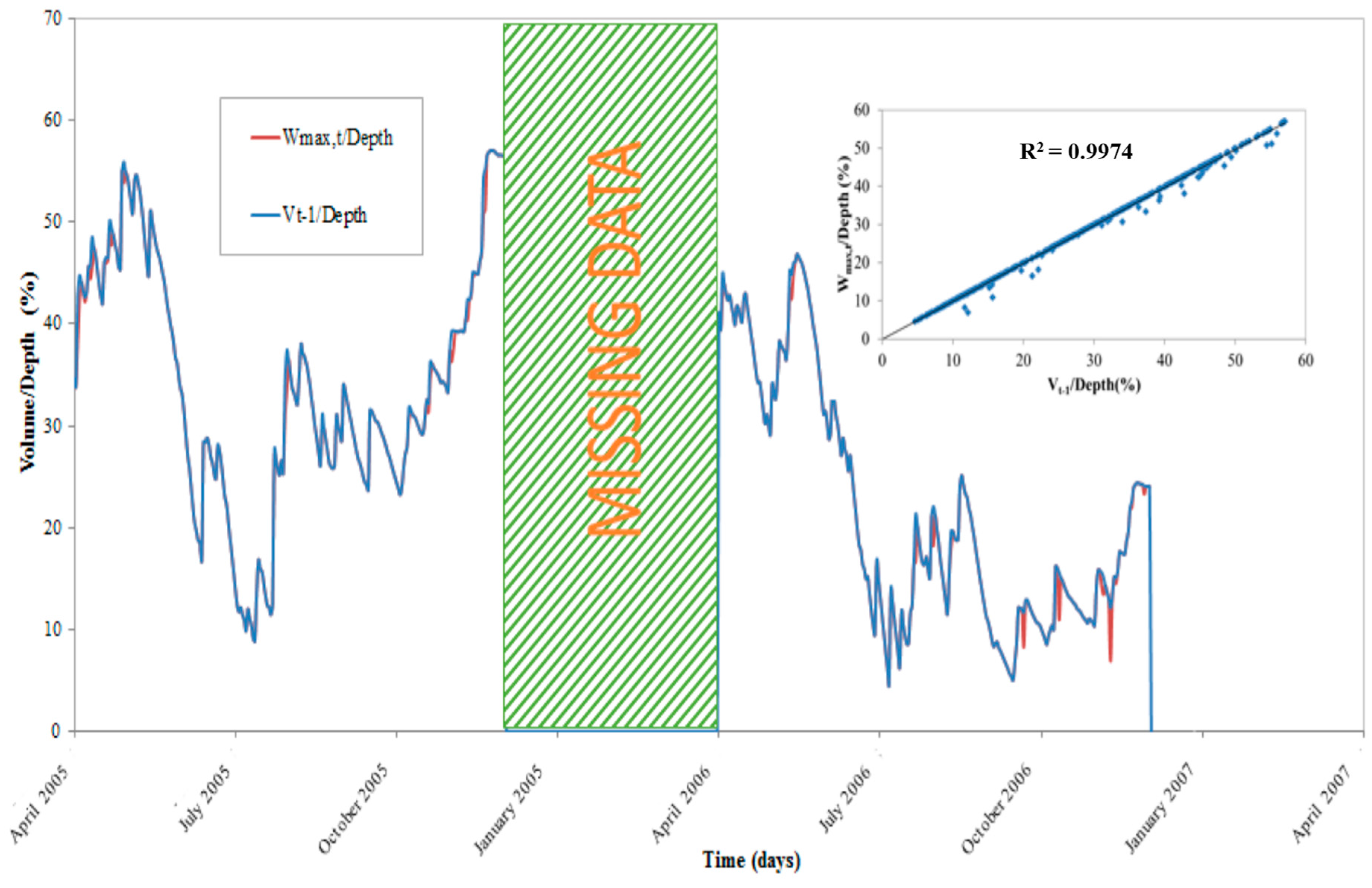
Figure A1, as a ratio of the green roof depth. Illustration refers to AET computed by the API method, but similar results are achieved for the AA method.
Figure A1.
Water depth (V) and water holding capacity (W) daily scale patterns as a ratio to soil depth. Actual evapotranspiration losses are computed by the API Method. Overlapped, in the upper right corner, the scatter plot for the two considered variables and the relevant Person correlation coefficient.
Considering the above discussed soil physical properties and also probably to balance the a-priori calculation for AET losses, W
max becomes a variable for the GR hydrological model itself. Its temporal pattern is nearly coincidental with the water depth pattern. Retention capacities approach a maximum value of about 55% during the rainy and cold seasons. They decline to about 10% during a short summer period, where the typical large amount of rainfall (high API values in
Figure 3) is contrasted by high evapotranspiration losses. In 2006, the retention capacity appears moderate also for the autumn season because of enhanced evapotranspiration losses compared to the same period of the previous year (
Figure 4 and
Table 1). Beyond the visual patterns coincidence, the coefficient of correlation between W
max,t and V
t−1 is extremely high (R
2 = 0.97). Thus, it can be reasonably assumed that:
Equation (13) becomes in the end:
References
- Hollander, J.B.; Pallagst, K.; Schwarz, T.; Popper, F.J. Planning shrinking cities. Prog. Plan. 2009, 72, 223–232. [Google Scholar]
- Fletcher, T.D.; Shuster, W.; Hunt, W.F.; Ashley, R.; Butler, D.; Arthur, S.; Trowsdale, S.; Barraud, S.; Semadeni-Davies, A.; Bertrand-Krajewski, J.L.; et al. SUDS, LID, BMPs, WSUD and more—The evolution and application of terminology surrounding urban drainage. Urban Water J. 2015, 12, 525–542. [Google Scholar] [CrossRef]
- Carter, T.; Jackson, C.R. Vegetated roofs for stormwater management at multiple spatial scales. Landsc. Urban Plan. 2007, 80, 84–94. [Google Scholar] [CrossRef]
- Vijayaraghavan, K. Green roofs: A critical review on the role of components, benefits, limitations and trends. Renew. Sustain. Energy Rev. 2016, 57, 740–752. [Google Scholar] [CrossRef]
- Carter, T.; Fowler, L. Establishing green roof infrastructure through environmental policy instruments. Environ. Manag. 2008, 42, 151–164. [Google Scholar] [CrossRef] [PubMed]
- Masseroni, D.; Cislaghi, A. Green roof benefits for reducing flood risk at the catchment scale. Environ. Earth Sci. 2016, 75, 1–11. [Google Scholar] [CrossRef]
- Versini, P.A.; Jouveb, P.; Ramierc, D.; Berthierc, E.; De Gouvelloa, B. Use of green roofs to solve storm water issues at the basin scale-Study in the Hauts-de-Seine County (France). Urban Water J. 2015, 13, 1–10. [Google Scholar] [CrossRef]
- Palla, A.; Gnecco, I.; Lanza, L.G. Hydrologic restoration in the urban environment using green roofs. Water 2010, 2, 140–154. [Google Scholar] [CrossRef]
- Longobardi, A.; Nazzareno, D.; Mobilia, M. Historical storminess and hydro-geological hazard temporal evolution in the solofrana river basin—Southern Italy. Water 2016, 8, 398. [Google Scholar] [CrossRef]
- Fletcher, T.D.; Herve, A.; Perrine, H. Understanding, management and modelling of urban hydrology and its consequences for receiving waters: A state of the art. Adv. Water Resour. 2013, 51, 261–279. [Google Scholar] [CrossRef]
- Sartor, J. The significance of the water balance in sustainable storm water management. In Flood Control Today—Sustainable Water Management; Erich Schmidt Publishers: Berlin, Germany, 2001; pp. 287–308. (In German) [Google Scholar]
- Mobilia, M.; Longobardi, A.; Sartor, J.F. Green Roofs Hydrological Performance under Different Climate Conditions. WSEAS Trans. Environ. Dev. 2015, 11, 264–271. [Google Scholar]
- Hilten, R.N.; Lawrence, T.M.; Tollner, E.W. Modeling storm water runoff from green roofs with HYDRUS-1D. J. Hydrol. 2008, 358, 288–293. [Google Scholar] [CrossRef]
- Yanling, L.; Babcock, R.W. A simplified model for modular green roof hydrologic analyses and design. Water 2016, 8, 343. [Google Scholar]
- Berthier, E.; De Gouvello, B.; Archambault, F.; Gallis, D. Water Balance of Green Roofs: Contributions to Better Understanding and Simulation; GRAIE: Lyon, France, 2010; Volume 6, pp. 39–47. [Google Scholar]
- Sherrard, J.; James, A.; Jennifer, M.J. Vegetated roof water-balance model: Experimental and model results. J. Hydrol. Eng. 2011, 17, 858–868. [Google Scholar] [CrossRef]
- Stovin, V.; Poë, S.; Berretta, C. A modelling study of long term green roof retention performance. J. Environ. Manag. 2013, 131, 206–215. [Google Scholar] [CrossRef] [PubMed]
- Jim, C.Y.; Peng, L.L.H. Substrate moisture effect on water balance and thermal regime of a tropical extensive green roof. Ecol. Eng. 2012, 47, 9–23. [Google Scholar] [CrossRef]
- Poë, S.; Stovin, V.; Berretta, C. Parameters influencing the regeneration of a green roof’s retention capacity via evapotranspiration. J. Hydrol. 2015, 523, 356–367. [Google Scholar] [CrossRef]
- Hardin, M.; Wanielista, M.; Chopra, M. A mass balance model for designing green roof systems that incorporate a cistern for re-use. Water 2012, 4, 914–931. [Google Scholar] [CrossRef]
- Hakimdavara, R.; Culligana, P.J.; Finazzia, M.; Barontinib, B.S.; Ranzib, R. Scale dynamics of extensive green roofs: Quantifying the effect of drainage area and rainfall characteristics on observed and modeled green roof hydrologic performance. Ecol. Eng. 2014, 73, 494–508. [Google Scholar] [CrossRef]
- Rheinland-Pfalz. Agrar Meteorologie. Available online: www.am.rlp.de (accessed on 21 July 2016).
- Yang, W.Y.; Li, D.; Sun, T.; Ni, G.H. Saturation-excess and infiltration-excess runoff on green roofs. Ecol. Eng. 2015, 74, 327–336. [Google Scholar] [CrossRef]
- Ali, M.F.; Mawdsley, J.A. Comparison of two recent models for estimating actual evapotranspiration using only regularly recorded data. J. Hydrol. 1987, 93, 257–276. [Google Scholar] [CrossRef]
- Gebler, S.; Hendricks Franssen, H.J.; Pütz, T.; Post, H.; Schmidt, M.; Vereecken, H. Actual evapotranspiration and precipitation measured by lysimeters: A comparison with eddy covariance and tipping bucket. Hydrol. Earth Syst. Sci. 2015, 19, 2145–2161. [Google Scholar] [CrossRef]
- Brutsaert, W.; Stricker, H. An advection-aridity approach to estimate actual regional evapotranspiration. Water Resour. Res. 1979, 15, 443–450. [Google Scholar] [CrossRef]
- Priestley, C.H.B.; Taylor, R.J. On the assessment of surface heat flux and evaporation using large-scale parameters. Mon. Weather Rev. 1972, 100, 81–92. [Google Scholar] [CrossRef]
- Allen, R.G.; Pereira, L.S.; Raes, D.; Smith, M. Crop Evapotranspiration-Guidelines for Computing Crop Water Requirements; FAO Irrigation and Drainage Paper 56; FAO: Rome, Italy, 1998. [Google Scholar]
- Marasco, D.E. Alternative Metrics of Green Roof Hydrologic Performance: Evapotranspiration and Peak Flow Reduction. Ph.D. Thesis, Columbia University, New York, NY, USA, 2014. [Google Scholar]
- Koehler, M.A.; Linsley, R.K. Predicting the Runoff from Storm Rainfall; U.S. Government Printing Office: Washington, DC, USA, 1951; pp. 1–10.
© 2017 by the authors. Licensee MDPI, Basel, Switzerland. This article is an open access article distributed under the terms and conditions of the Creative Commons Attribution (CC BY) license ( http://creativecommons.org/licenses/by/4.0/).


