Discharge Measurements of Snowmelt Flood by Space-Time Image Velocimetry during the Night Using Far-Infrared Camera


Department of Civil Engineering, Graduate School of Engineering, Kobe University, Kobe 657-8501, Japan
Water 2017, 9(4), 269; https://doi.org/10.3390/w9040269
Submission received: 12 December 2016
/
Revised: 6 April 2017
/
Accepted: 7 April 2017
/
Published: 11 April 2017
(This article belongs to the Special Issue Advances in Hydro-Meteorological Monitoring)
Abstract
:The space time image velocimetry (STIV) technique is presented and shown to be a useful tool for extracting river flow information non-intrusively simply by taking surface video images. This technique is applied to measure surface velocity distributions on the Uono River on Honshu Island, Japan. At the site, various measurement methods such as a radio-wave velocity meter, an acoustic Doppler current profiler (ADCP) or imaging techniques were implemented. The performance of STIV was examined in various aspects such as a night measurement using a far-infrared-ray (FIR) camera and a comparison to ADCP data for checking measurement accuracy. All the results showed that STIV is capable of providing reliable data for surface velocity and water discharge that agree fairly well with ADCP data. In particular, it was demonstrated that measurements during the night can be conducted without any difficulty using an FIR camera and the STIV technique. In particular, using the FIR camera, the STIV technique can capture water surface features better than conventional cameras even at low resolution. Furthermore, it was demonstrated that measurements during the night can be conducted without any difficulty.
1. Introduction
Intensive and record-breaking rainfall caused severe flood disasters in the world and in Japan in recent years partially due to the global warming [1]. For example, in July 2011, Niigata and Fukushima areas suffered from torrential rain with levee breaches and inundation disasters at many locations due to the maximum flood in recorded history. In September 2011, typhoon No. 12 directly hit Nara and Wakayama Prefectures causing landslide and sediment-related disasters in a wide area. Furthermore, in July 2012, a total of eight first-class river systems in the northern part of Kyushu Island were severely damaged twice by a torrential rain brought by a seasonal rain front. In 2015, the Kinugawa River, a first-class river in Kanto area, suffered from a levee breach, causing a huge inundated area while destroying nearby houses. In the Japanese river management system, 109 rivers are designated as first-class rivers, for which the Japanese government is responsible for the management of major river reach. The other smaller rivers of more than four thousand are classified as second-class rivers, for which the local government takes care of the river reach.
It should also be mentioned that huge flood disasters are taking place every year in the world; e.g., Australia, Brazil, China and Thailand were struck by a record-breaking flooding in the past decades [2]. A specific feature of the recent flood is characterized by the fact that heavy rain with an hourly rainfall intensity of about 100 mm continues for several hours, and this causes a sudden increase of river discharge, which results in an inundation in the worst case. In order to be prepared for such disasters, it is of vital importance to collect and analyze hydrological data such as rainfall intensity, water level and flow discharge. The acquisition of such data is important for the purpose of understanding rainfall run-off processes correctly while tuning various parameters included in a run-off model [3,4]. Among the hydrological data, peak discharge is the most important information because it can determine the flow capacity of a river section in response to a heavy rainfall. However, contrary to the floods in continental large-scale rivers, which last several days or weeks, typical floods in Japan have a duration of several hours; therefore, it becomes difficult to correctly measure the flow at the right timing especially when the peak flow occurs during the night time. In the past, discharge measurements in Japan have been conducted mainly by using a float [5] with its length dependent on the water depth. In Japan, float is made of cardboard pipe in which a certain amount of sand is contained to control its specific gravity close to unity when it floats. According to the Japanese regulation, floats with different lengths are used depending on the water depth; e.g., two-meter float is used when the water depth is greater than 2.6 m and less than 5.2 m.
However, there exist several critical defects in this method because a measurement site of a bridge can be submerged in a huge flood, as actually occurred in the 2011 Niigata Flood. In this case, the measurement itself became impossible and one missed a chance to measure the peak flow. Furthermore, the road to the measurement site was closed due to inundation. In the case of the flood of Kyushu in 2012, the water level rose to the height of the river bank and overflowing flooding actually occurred. Particularly in the dark night time, it is difficult to apply the float method as the measurement might become dangerous in such a condition. In addition, even if measurement is possible, the float may seriously meander under the influence of large-scale river turbulence, which may greatly reduce measurement accuracy.
In the light of such a present status of discharge measurement, the so-called non-intrusive measurement techniques have been paid attention to in recent years, such as a radio-wave velocity meter (RVM) [6,7] or imaging techniques [8,9,10,11,12]. The RVM is usually installed at a bridge to measure streamwise surface velocity continuously at one point by using the effect of the Doppler shift of the surface flow [6,7]. However, the instrument has to be shifted back and forth along the bridge when trying to measure a cross-sectional velocity distribution or a large number of the instruments have to be installed along a bridge with a high cost. An alternative method is the use of surface-flow video images taken from a river bank. The idea behind the use of video images is that surface flow features composed of surface ripples or floating objects are assumed to be advected with the surface velocity as long as the wind effect is negligible. Among the image-based techniques, such as a large-scale image velocimetry (LSPIV) [13,14,15] or the space-time image velocimetry (STIV) [16,17,18,19,20], STIV seems to be more robust under deteriorated image condition and utilized in the present research. The non-intrusive methods are very useful and effective as they can measure the flow velocity information safely from a remote place. However, the image obtained by a conventional video camera has a shortcoming incapable of recording favorable images during the night. Since peak flows frequently occur in a dark condition in Japan, the existing river monitoring systems’ installed conventional cameras are difficult to use for flow measurements. In order to overcome this weak point, we propose a method to use a far-infrared ray (FIR) camera in river flow measurements. It is worth mentioning that traditional invasive instruments such as propeller ammeters, electromagnetic flowmeters or ADCP cannot be applied during high-speed floods. On the other hand, STIV, for example, can measure velocities over 5 m/s [16]. In this paper, we examined the traceability of the surface texture composed of surface ripples without tracers to the surface flow, and discussed the measurement accuracy of river flow rate by using the image obtained by the FIR camera. Furthermore, robustness of the STIV technique to LSPIV in measuring streamwise velocity components when using deteriorated images of low resolution will be shown.
2. Outline of Space-Time Image Velocimetry
2.1. Image Rectification by Camera Calibration and Search Lines
STIV is an image analysis technique to measure streamwise water surface velocity distributions from video images usually taken from a riverbank. This technique assumes that features that appeared on the water surface would follow the surface velocity when the wind effect is negligible. The idea to use surface feature advection is the same as the radio-wave velocity meter or LSPIV. The aspect of STIV different from the other techniques is that STIV pays attention to the time- and space-averaged velocity along a line segment set in the streamwise direction. The line segment is treated as a search line for velocity estimation.
In the first step of STIV, establishing a relation between the screen coordinates (x, y) and the physical coordinates (X, Y, Z), by using the following collinearity equation is required:
where c is the focal distance, aij with 1 ≤ i ≤ 3 and 1 ≤ j ≤ 3 are mapping coefficients, (X0, Y0, Z0) is the physical coordinates of the camera, and (x0, y0) is the center of the screen image. The coefficients can be determined via a camera calibration procedure by using at least six ground control points. The image rectification can be performed by substituting the water level data H to Z in the above equations. An example of the image rectification for an image obtained by using a normal high definition video camera is shown in Figure 1, together with the search lines set parallel to the streamwise direction. The length of the search line is 17.6 m and the transverse spacing is 5.6 m in this case. The set of search lines covers almost the whole width of the river of 140 m. The direction of search lines is determined by visual inspection after generating a rectified image, i.e., the lines are drawn parallel to the riverbank.
2.2. Space Time Image
After the set of search lines, space time images (STIs) are generated for each search line by taking brightness distribution in the search line as the horizontal axis and its evolution with time as the vertical axis. Several examples of STI in a transverse direction is shown in Figure 2. The horizontal length is 17.6 m and the downward vertical axis is ten seconds. Since the frame rate of image sampling is 30 frames per second, the vertical length is composed of 300 images. The images are enhanced for a better recognition of surface features by applying the histogram equalization technique. It is clearly seen that an inclined pattern is generated in each STI, indicating that overall surface features are advected along the search line with the flow at almost constant speed, although there are some other noisy patterns created by surface wave motion moving in the direction different from the main flow. The average gradient of the pattern corresponds to the local time- and space-averaged mean velocity along the search line.
2.3. Measurement of Orientation Angle of the Pattern
In the original STIV, the average orientation angle f of a STI is obtained by dividing the STI into small segments and calculating the local gradient for each segment as indicated in Figure 3. The local orientation angle φ can be calculated using the following relations [17]:
where
g(x,t) is the grey level intensity in STI and A is the area of the small segment indicated in Figure 3a. Typically, A is a square with a side length of fifteen pixels. Figure 3b provides a distribution of the coherency defined by
which is a measure of the image pattern coherence and takes a value between zero and one; for an ideal local orientation, its value becomes one, and, for an isotropic gray image, it becomes zero. Therefore, it is possible to calculate the mean orientation angle by preferably obtaining clearer orientation information by taking coherency as a weighting function:
Figure 3c is a weighted histogram of the orientation angle, showing a distribution with a peak. Since the length and time scales of the STI are given, the mean velocity along the line segment can be calculated by the following relation:
where Sx is the unit length scale along the search line (m/pixel) and St is the unit time scale of the time axis.
3. Outline of the Field Measurement
3.1. Study Area
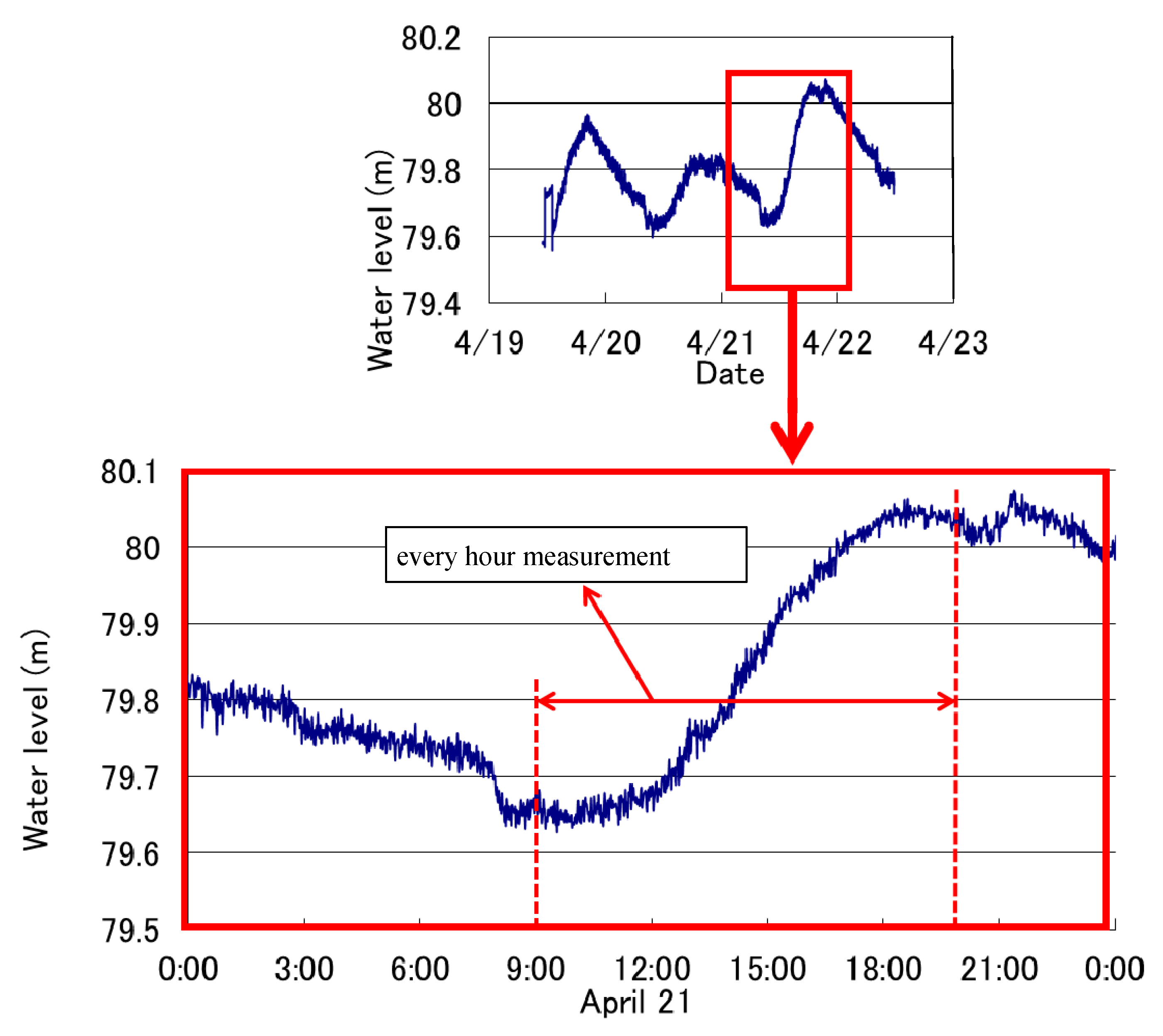
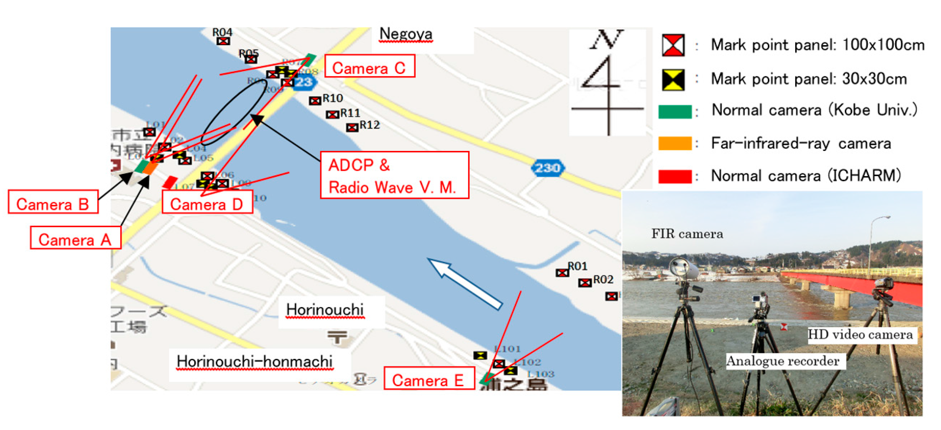
Field investigations were conducted from 19 April to 22 April in 2012 at the Negoya Bridge of the Uono River, which is a major tributary of the Shinano River, the longest river in Japan. The site is located at Horinouchi in Uonuma City of Niigata Prefecture in the middle of Japan. This location was chosen because daily snowmelt flood occurs frequently in early spring, and we could actually observe the increase of water level of about 40 cm due to the snowmelt during our measurements every day as shown in Figure 4. The water level sensor of a pressure type was temporally installed near the panel R04 (Figure 5). On the measurement day, the water level rose up to the full width of the lower channel with a width of about 150 m, while the bank to bank width is about 220 m. The measurements were mainly conducted at the cross-section downstream of the bridge every hour in order to compare the performance of various measurement methods, i.e., STIV with normal cameras, STIV with a FIR camera, RVM, and an ADCP. Floats were also supplied from the bridge to compare their velocity with the surface velocity measured by the above methods. Figure 5 is the measurement site showing the location of cameras and mark point panels to be used for a camera calibration in STIV measurement. The panels were carefully set so that at least six of them are visible for each camera screen. The measurements were conducted jointly with staffs from International Centre for Water Hazard and Risk Management (ICHARM) under the auspices of UNESCO and several consulting companies.
3.2. Image Acquiring Methods
In the present observation, several cameras took images of the water surface from various angles. The cameras are an FIR camera (Camera A in Figure 4) and four normal high-definition video cameras (cameras B to E). Cameras A, B and C viewed the same water surface zone downstream of the bridge where ADCP and radio-wave measurements were executed. Camera D and Camera E took images just upstream and far upstream of the bridge, respectively. Figure 5 shows how the measurement were conducted at the site. It shows that the image-based measurement technique is quite simple, i.e., just take surface images from a riverbank, taking care about the size of the field of view. The important point is to set at least six ground reference points (GRPs) within the field of view for the ortho-rectification of images.
The measurements were repeated every hour for about five minutes from 10:00 a.m. to 8:00 p.m. The FIR camera (FLIR Systems, SR-334, Wilsonville, OR, USA), has a resolution of 320 by 240 pixels and its image sampling frequency is 7.5 fps, while normal high definition (HD) cameras have a resolution of 1920 by 1080 pixels with 30 fps. The video images of the FIR camera were recorded as an NTSC (National Television System Committee) format on an analogue video recorder with a size of 640 by 480 pixels at 30 fps as indicated in Figure 4. Therefore, the recorded images were somewhat blurred with a staggering frame sequence. The relationship between the screen and physical coordinates were determined from the location of mark point panels for each coordinate. Typical panels are made of plywood with a size of 1 m by 1 m. As the resolution of the FIR camera is not high, and, at the same time, it was difficult to detect the panels on the other side of the river about 150 m away from the camera, pocket heating pads were attached on the panel for improving the visibility of panel locations. Since the air temperature is very low (about 5 °C), heated spots were clearly visible in FIR camera screen even from a distant location.
3.3. Comparison of Captured Images
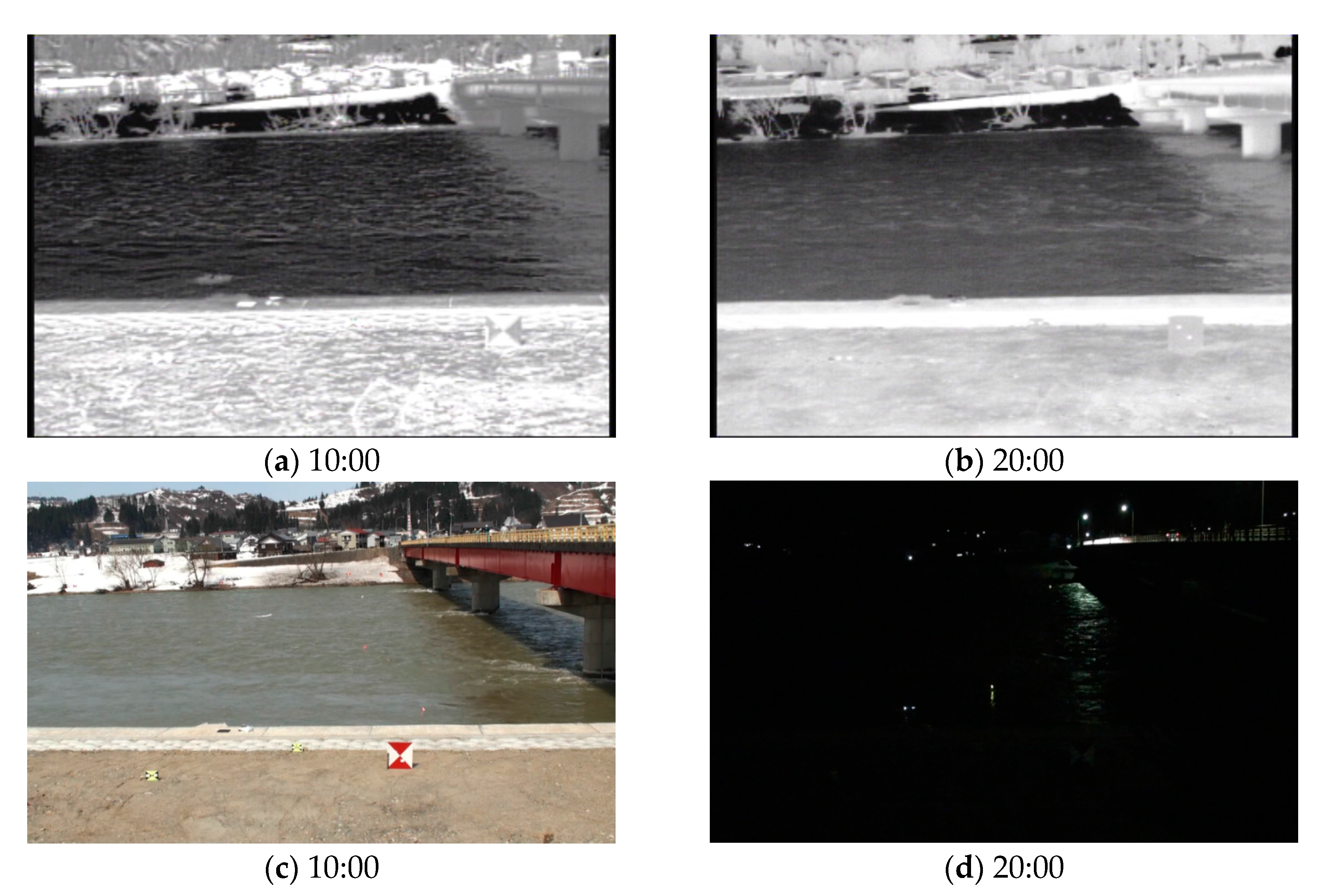
In order to demonstrate the interest of a FIR camera for river flow measurement, images captured in the morning and at night are compared in Figure 6 together with the images captured by a normal camera. It is obvious from the upper images in Figure 6 that the FIR camera can capture the river surface pattern clearly even during the night with low light condition, while a normal camera can recognize only the water surface just beneath street lamps at the bridge as indicated in lower left image in Figure 6. It can be considered that an FIR camera senses only the heat differences of objects, but the intensity of the received infrared ray changes depending on the slope of reflected surface even when the object temperature is the same. It should be noted that the original image size is only 320 by 240 pixels in FIR compared with the normal image size of 1920 by 1080 pixels. Although the surface pattern by FIR camera seems to be rather smoothed out in the night image as seen in Figure 6b, advection of the pattern in the downstream direction was observed in STI, which is a significant advantage over conventional cameras when developing a real-time measurement system using STIV.
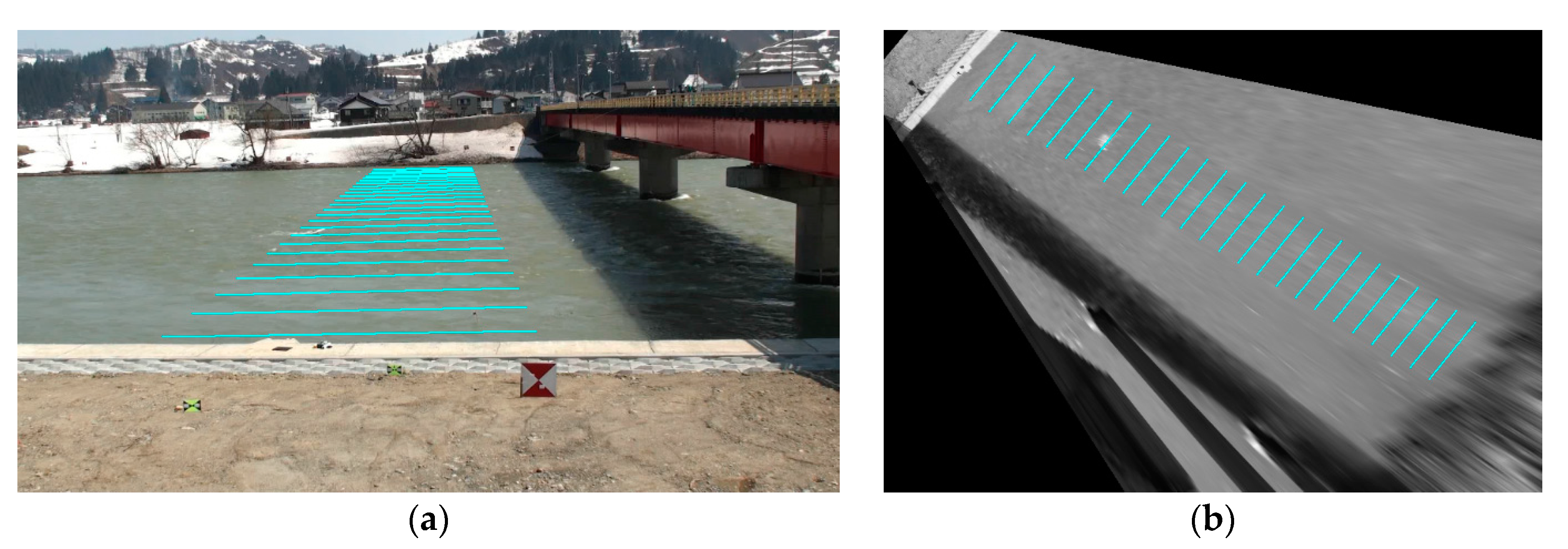
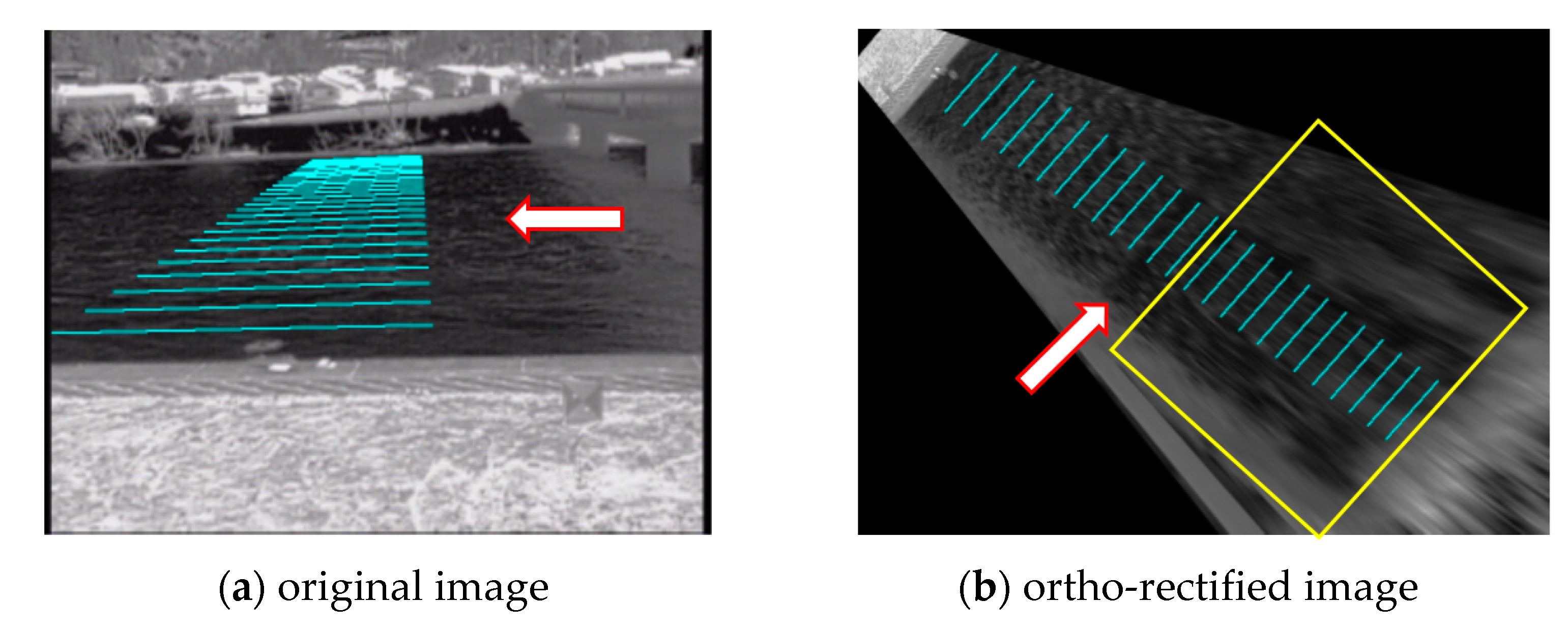
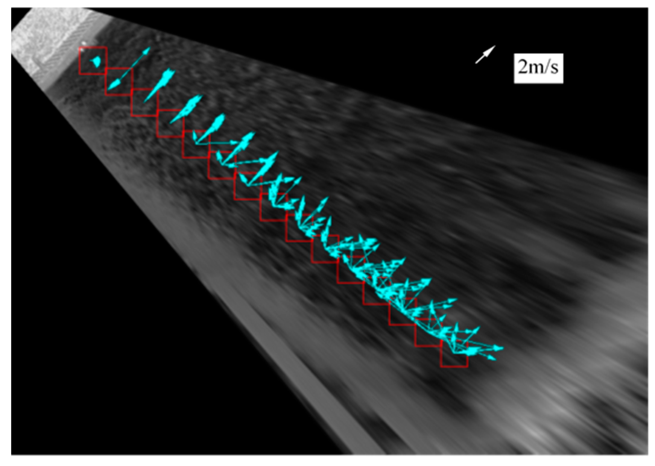
Figure 7 shows 25 search lines set on oblique and rectified images for the FIR camera A. The search lines were drawn parallel to the river bank at an equal spacing in a similar manner indicated in Figure 1. Its length is 17.8 m and the spacing is 5.7 m, covering the river width of about 140 m. It can be noted in Figure 7b that the image texture within a rectangle region becomes significantly blurred after the ortho-rectification. This is because the pixel image is greatly expanded for the region far from the camera location. As an example, the original spatial resolution along the farthest search line is 33.6 cm/pixel in this case, which is a very large value trying to reproduce the actual water surface roughness pattern. Because of this insufficient information of image texture in that region, it was difficult to apply LSPIV to the whole width since LSPIV uses a pattern matching technique to track the surface texture. As an example, Figure 8 provides the results by LSPIV applied to sequential ortho-rectified images such as shown in Figure 7b. The images ortho-rectified with a pixel size of 0.2 m and a time interval of 0.133 seconds were used for the analysis. The template size for the pattern matching in PIV was set at 33 by 33 pixels, which is 6.6 by 6.6 m in physical scale. In Figure 8, instantaneous vectors are superposed to show variations in data. It is obvious that variation in data increases significantly with the distance from the left bank where the FIR camera is located. Since the actual flow direction is almost unidirectional, the scatter in the data is unreliable. This is because the image is largely stretched in the transverse direction in the process to ortho-rectification. On the other hand, the data nearer to the left bank shows almost uniform variation, indicating that reliable data are obtained only until about half-width, i.e., about 70 m, from the left bank. This feature suggests that the flow rate cannot be analyzed from the LSPIV in the cases where the image resolution is low and the image stretching becomes large in the image transformation, such as in the present situation.
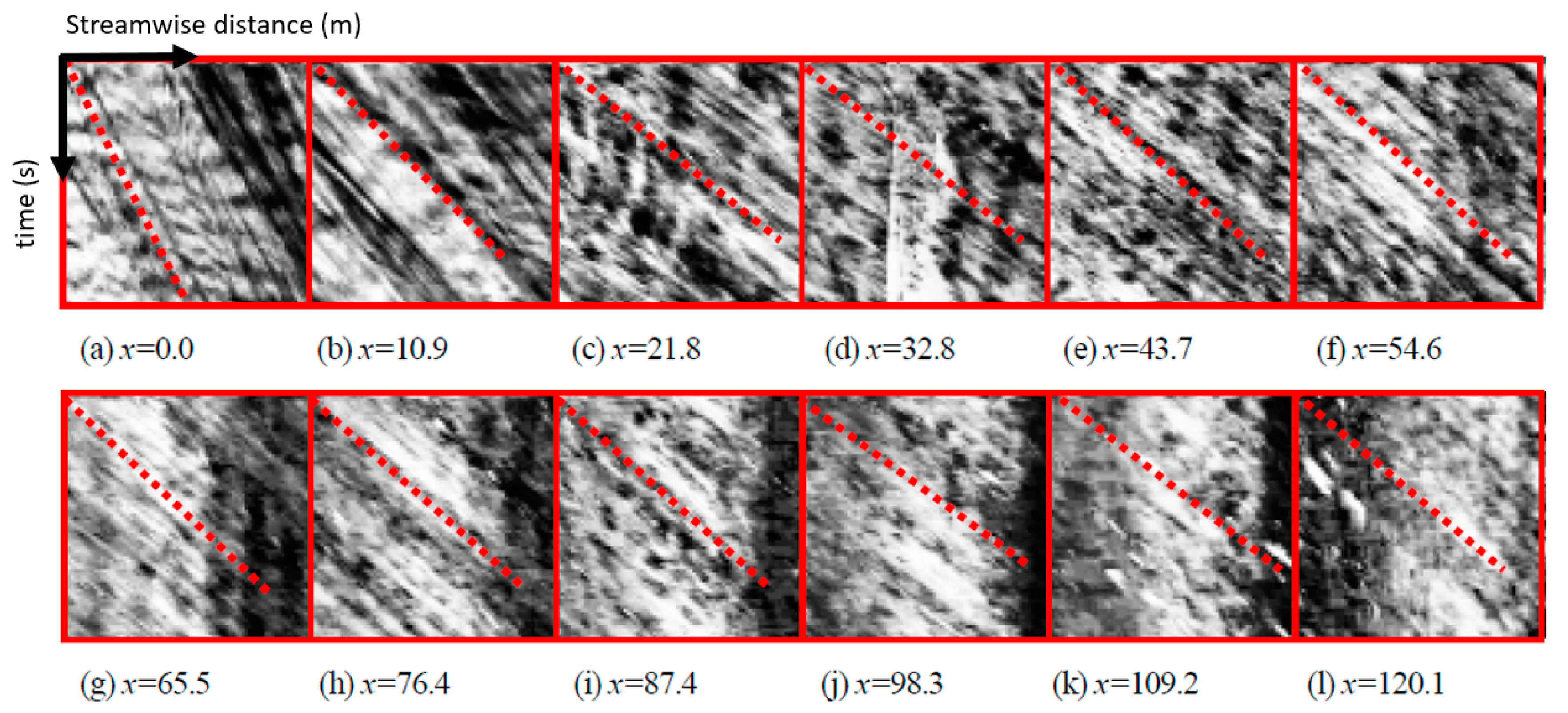
In order to show good sensitivity when using spatiotemporal images, Figure 9 shows the STI obtained by the FIR camera at almost the same position as the STI shown in Figure 2 obtained by a high resolution camera. The images are enhanced by the same technique as for Figure 2. Although the FIR camera used in the measurement have only one sixth of the resolution of the high definition camera, similar patterns appear in the resulting STIs even at the farther locations from the camera location. This feature of STI is the source of robustness in applying STIV to various types of flood flows [16].
3.4. Traceability of Water Surface Features
In using non-contact techniques for surface flow measurement such as RVM, LSPIV or STIV, water surface features generated by turbulence are assumed to be advected with the surface flow velocity as previously mentioned. In order to validate this assumption, an STI for the search line intentionally set along a trajectory of a float captured by camera B is shown in Figure 10 together with an STI by an FIR camera for the same location. The trajectory of the float is visible as a straight line as seen in Figure 10a, indicating that the float moved at a constant speed along the search line, from which its speed can be easily obtained from the slope of the trajectory. In Figure 10a, there appears a texture almost parallel to the float trajectory. An STI at the same location obtained by an FIR camera is shown in Figure 10b. The important point is that the gradient of the oblique patterns obtained by the two cameras is almost the same as that of the float trajectory. Referring to the four straight lines of the same gradient superposed in the figures, a good agreement of the speeds can be visually recognized, indicating the traceability of surface features to the surface flow.
Another example for examining traceability of surface features is shown in Figure 11, which compares a trajectory of a piece of driftwood and surface features. Since these STIs are obtained from the camera D located upstream of the bridge, surface features displays straight uniform patterns. This is because the water surface was not disturbed by the pier of the bridge as in the downstream region. The trajectory of driftwood coincides with the surface pattern gradient so that it seems to be embedded in the pattern. This suggests that measurements by STIV should be conducted on the upstream side of the bridge, without disturbance by the bridge pier
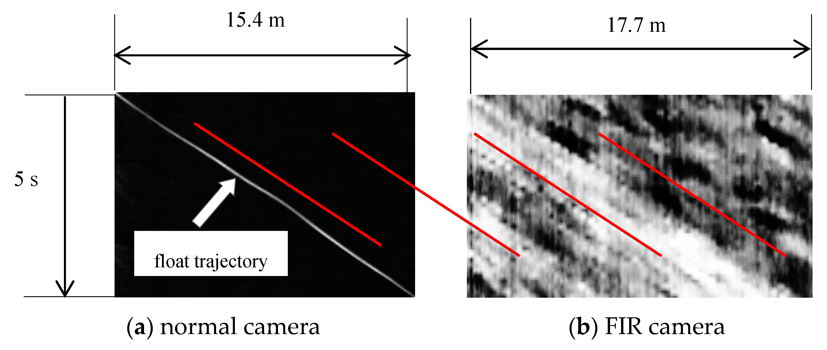
Finally, Figure 12 compares the trajectory of a luminous float on the STI captured by a normal camera and STI by an FIR camera obtained at night. The luminous float is used conventionally in a dark condition in Japan. It has a fluorescent part at the top of the normal float so that an observer can easily detect the light from the river bank. Again, due to the low spatial resolution of the FIR camera used in the present study, oblique patterns displayed in Figure 12b do not have sharp outlines, but it is possible to determine the slope of the general pattern even in such a deteriorated image condition. Referring to the parallel lines drawn in the figure, the gradient of the light trajectory agrees quite well with the pattern slope by the FIR camera. Therefore, the conventional measurement during the night by using a luminous float can be replaced by STIV using an FIR camera. In this respect, STIV is much more robust than LSPIV in which a reliable matching of image pattern has to be established in a sub-pixel level. Alternatively, STI containing a float trajectory, such as indicated in Figure 12a, can be used for STIV measurement when an FIR camera is not available. The gradient of the pattern can be obtained either manually or automatically with the aid of an STIV algorithm [17].
4. Results and Discussion
4.1. Comparison with Other Measurement Methods
As mentioned previously, the measurements were conducted every hour from 10:00 a.m. to 8:00 p.m. During the measurements, the water level rose about 50 cm due to the melting of snow from the mountainous region. The water level repeated up and down changes due to the snowmelt in the daytime as has been indicated in Figure 5. Figure 13 shows surface velocity distributions downstream of the Negoya Bridge at 1:00 p.m. and 8:00 p.m. measured by various methods, i.e., STIV by the far infrared camera on the left bank, STIVs by normal camcorders on the left and the right banks, a radio-wave velocity meter, and an ADCP. The cross-sectional bottom shape measured by ADCP was also indicated in the figure.
As for the ADCP data, the streamwise velocity component closest to the water surface, about 30 cm below it, were compared as representing the surface velocity. Since the ADCP measurement is conducted by tagging the boat-mounted sensor manually in a transverse direction, the data indicated are almost instantaneous values and have a great scatter especially in the region downstream of the bridge piers, where large-scale unsteady wake flow is generated. On the other hand, measurements by a radio-wave velocity meter were conducted by shifting its position step by step manually along the bridge. It measures a locally averaged velocity within a circular spot with a diameter of a few meters on the water surface by utilizing the Doppler shift effect. The obtained data falls into a scattered range of ADCP data.
Regarding the measurements by STIV, plots by the normal video cameras and the FIR camera show a large scatter within the wake flow region with the maximum relative error more than 0.5 m/s as shown in Figure 13a. Compared to the ADCP data, the FIR camera produced a favorable velocity distribution with a relative error of about 10%, which also agreed well with the RVM data. Since normal cameras are impossible to use at night, STIV by the FIR camera are compared with ADCP and RVM as shown in Figure 13b. Keeping in mind the scatter in ADCP data, data by the FIR camera agrees quite with the other data with a relative error of about 10%.
Comparing the STIV data obtained by normal video cameras and the FIR camera, normal cameras record the light reflection from the water surface roughness while the FIR camera mainly detects the temperature difference as well as the radiation intensity that varies with the roughness shape. Since the spatial resolution along a search line decreases with the distance from the camera, there should be some limitation in terms of the width of the river that STIV can be applicable. According to the author’s experience, the present case with a width of about 150 m might be the maximum distance at which STIV can yield reliable data.
Regarding the transverse bed profile at the section downstream of the bridge shown in Figure 13, the river bed is deeper closer to the left bank and a ridge-like deposition occurs downstream of a bridge pier. Another lower deposition can be found closer to the right bank just after the other bridge pier. Generally speaking, water surface velocity distributions measured by the above methods agree well with each other in the entire cross-section with its distribution influenced by the bottom variation, i.e., faster in a deeper zone and slower in a shallower part. The maximum velocity occurred near the left bank increased from about 2.8 m/s at 1:00 p.m. to about 3.3 m/s at 8:00 p.m. due to the increase of discharge.
In order to examine the effect of the bridge piers that disturb the surface features, time variation of velocity distributions measured by STIV with Camera D just upstream of the Negoya Bridge is shown in Figure 14. The location of the Camera D is indicated in Figure 4. As can be seen from Figure 10 obtained at the upstream section, the oblique patterns that appeared on the STI show continuous straight features with little disturbance, indicating that surface features are advected steadily at a constant speed without the influence of hydraulic structures. As a result, the transverse velocity distributions are much smoother than that shown in Figure 13. This feature is important for improving the measurement accuracy by STIV. Unfortunately, we could not calculate the flow rate because the riverbed shape of this section was unknown, but once the topographic data is available, more reliable discharge data could be obtained.
4.2. Discharge Measurement Accuracy
Figure 15 compares a discharge directly measured by ADCP and estimated discharges from surface velocity distributions by STIV and a radio-wave velocity meter. In integrating the velocity distribution measured by ADCP, the surface velocity Us was assumed to be the same as the data 30 cm below the water surface. In using STIV, discharge was obtained by dividing the river width by the interval of the search line Δyi, multiplying the flow velocity at the search line by a surface velocity ratio α, the local flow depth hi, and finally summing the piecewise discharges. Therefore, the discharge can be calculated by the following formula:
Similar flow rate calculation is also performed by RVM, but the number of measurement cross-sections by STIV was much larger than RVM; i.e., 25 sections in STIV and eight sections in RVM. In STIV, the number of sections can be increased easily, but it becomes physically difficult to conduct a simultaneous measurement in using RVM. In the present discharge calculation shown in Figure 14, the conventional value of 0.85 was used for α, and, as a result, underestimated values were obtained when compared to ADCP data. Therefore, using a value of 0.9 for α would increase the degree of coincidence at the section downstream of the bridge. As shown in Figure 14, even with a value of 0.85 for α, the relative error is less than ten percent, which is acceptable in the practical usage of STIV.
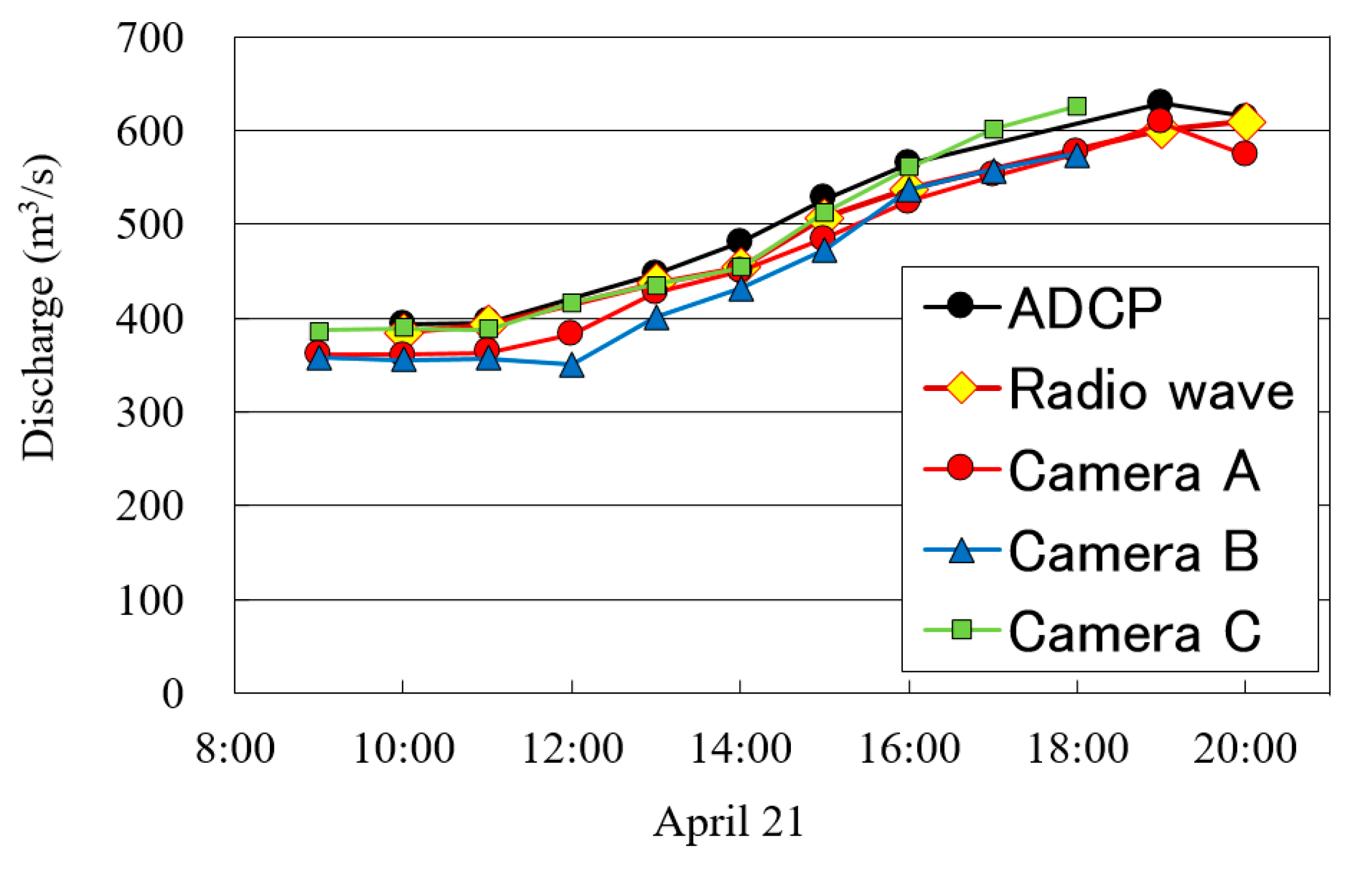
Figure 16 compares the discharge hydrographs obtained by the above methods. The discharge increased about 200 m3/s due to the snowmelt. The discharge began to increase just after noon, reached its peak at 7:00 p.m. and decreased again after that, which indicates a typical feature of snowmelt flood in Japan.
5. Conclusions
Velocity fields of the snowmelt flood that occurred in the Uono River were measured by various cutting-edge methods such as imaging techniques, ADCP and radio-wave velocity meter. Among them, imaging techniques used to be considered difficult to apply during the night. However, this shortcoming was overcome by introducing a far-infrared ray camera in the present study for the first time for flood flow measurement with surface velocities more than 3 m/s. Puelo et al. [21] used a thermal infrared camera to measure small stream flows, but the velocity level was low with the maximum velocity less than 0.9 m/s, and it was not a flood measurement. Regarding the traceability of surface features, the assumption that surface features are advected with the surface velocity was verified by directly comparing it with the velocities of floating objects such as driftwood or floats in a space-time image. It was also made clear that the measurement accuracy of discharge by STIV was comparable to the direct measurement by ADCP with a relative error less than ten percent. In the actual situation of discharge measurements, measurement sections should have to be located upstream of a bridge because surface features at the downstream section can be destroyed by wake flows generated at the piers. Regarding the use of LSPIV, another widely-used image-based technique, it yielded erroneous values where the stretching of the image in the transverse direction is remarkable. On the other hand, STIV yielded stable results even where the image resolution and quality is low farther from the camera location. In that sense, STIV is a promising technique for measuring river discharges safely from a remote place even for an overtopping flood flow. However, the conventional surveillance camera such as closed-circuit television (CCTV) is difficult to use at night with little surrounding light. Therefore, an FIR camera is recommended for establishing a real-time measurement system that works all the time. Further investigation is required to examine the effects of strong wind or heavy rain on the accuracy of STIV measurements.
Acknowledgments
The study was supported by a research grant from the Foundation of River and Basin Integrated Communications (FRICS) Foundation in collaboration with ICHARM. The data other than imaging data were provided through ICHARM. I am grateful to their support of the present research.
Conflicts of Interest
The author declares no conflict of interest.
Abbreviations
The following abbreviations are used in this manuscript:
| ADCP | Acoustic Doppler Current Profiler |
| RVM | Radio-wave Velocity Meter |
| FIR | Far-Infrared Ray |
| ICHARM | International Centre for Water Hazard and Risk Management |
| LSPIV | Large Scale Particle Image Velocimetry |
| STIV | Space Time Image Velocimetry |
| STI | Space time image |
| CCTV | Closed-circuit television |
References
- Schiermeier, Q. Increased flood risk linked to global warming: Likelihood of extreme rainfall may have been doubled by rising greenhouse-gas levels. Nature 2011, 470, 316. [Google Scholar] [CrossRef] [PubMed]
- Okazumi, T.; Nakasu, T. Lessons learned from two unprecedented disasters in 2011—Great East Japan Earthquake and Tsunami in Japan and Chao Phraya River flood in Thailand. Int. J. Disaster Risk Reduct. 2015, 13, 200–206. [Google Scholar] [CrossRef]
- Xu, G.-Y. Climate change and hydrologic models: A review of existing gaps and recent research developments. Water Resour. Manag. 1999, 13, 369–382. [Google Scholar] [CrossRef]
- Moradkhani, H.; Sorooshian, S. General review of rainfall-runoff modeling: Model calibration, data assimilation, and uncertainty analysis. Hydrol. Model. Water Cycle 2009, 63, 1–24. [Google Scholar]
- Turnipseed, D.P.; Sauer, V.B. Discharge Measurements at Gaging Stations. U.S. Geological Survey Techniques and Methods Book 3; USGS: Reston, VA, USA, 2010; Chapter 8; p. 87.
- Fukami, K.; Yamaguchi, T.; Imamura, H.; Tashiro, Y. Current status of river discharge observation using non-contact current meter for operational use in Japan. World Environ. Water Resour. Congr. 2008, 2008, 1–10. [Google Scholar]
- Welber, M.; Le Coz, J.; Laronne, J.B.; Zolezzi, G.; Zamler, D.; Dramais, G.; Hauet, A.; Salvaro, M. Field assessment of non-contact stream gauging using portable surface velocity radars (SVR). Water Resour. Res. 2016, 52, 1108–1126. [Google Scholar] [CrossRef]
- Fujita, I.; Komura, S. Application of video image analysis for measurements of river surface flows. Proc. Hydraul. Eng. JSCE 1994, 38, 733–738. (In Japanese) [Google Scholar] [CrossRef]
- Fujita, I.; Muste, M.; Kruger, A. Large-scale particle image velocimetry for flow analysis in hydraulic engineering applications. J. Hydraul. Res. 1998, 36, 397–414. [Google Scholar] [CrossRef]
- Muste, M.; Fujita, I.; Hauet, A. Large-scale particle image velocimetry for measurements in riverine environments. Water Resour. Res. 2008, 44, W00D19. [Google Scholar] [CrossRef]
- Muste, M.; Hauet, A.; Fujita, I.; Legout, C.; Ho, H.-C. Capabilities of Large-scale Particle Image Velocimetry to characterize shallow free-surface flows. Adv. Water Res. 2014, 70, 160–171. [Google Scholar] [CrossRef]
- Hauet, A.; Creutin, J.-D.; Belleudy, P. Sensitivity study of large-scale particle image velocimetry measurement of river discharge using numerical simulations. J. Hydrol. 2008, 349, 178–190. [Google Scholar] [CrossRef]
- Jodeau, M.; Hauet, A.; Paquier, A.; Le Coz, J.; Dramais, G. Application and evaluation of LS-PIV technique for the monitoring of river surface velocities in high flow conditions. Flow Meas. Instrum. 2008, 19, 117–127. [Google Scholar] [CrossRef]
- Dramais, G.; Le Coz, J.; Camenen, B.; Hauet, A. Advantages of a mobile LSPIV method for measuring flood discharges and improving stage–discharge curves. J. Hydro-Environ. Res. 2011, 5, 301–312. [Google Scholar] [CrossRef]
- Le Coz, J.; Hauet, A.; Pierrefeu, G.; Dramais, G.; Camenen, B. Performance of image-based velocimetry (LSPIV) applied to flash-flood discharge measurements in Mediterranean rivers. J. Hydrol. 2010, 394, 42–52. [Google Scholar] [CrossRef]
- Fujita, I.; Kumano, G.; Asami, K. Evaluation of 2D river flow simulation with the aid of image-based field velocity measurement techniques. In River Flow 2014; Schleiss, A.J., Cesare, G.D., Franca, M.J., Pfister, M., Eds.; Taylor & Francis Group: London, UK, 2014; pp. 1969–1977. [Google Scholar]
- Fujita, I.; Watanabe, H.; Tsubaki, R. Development of a non-intrusive and efficient flow monitoring technique: The space time image velocimetry (STIV). Int. J. River Basin Manag. 2007, 5, 105–114. [Google Scholar] [CrossRef]
- Tsubaki, R.; Fujita, I.; Tsutsumi, S. Measurement of the flood discharge of a small-sized river using an existing digital video recording system. J. Hydro-Environ. Res. 2011, 5, 313–321. [Google Scholar] [CrossRef]
- Fujita, I.; Hara, H. Development of space time image velocimetry introduced fast Fourier transform for improving robustness in river surface flow measurement. J. Hydrosci. Hydraul. Eng. 2011, 29, 123–135. [Google Scholar]
- Fujita, I.; Kosaka, Y.; Yorozuya, A.; Motonaga, Y. Surface flow measurement of snow melt flood using a far infrared camera. J. Jpn. Soc. Civ. Eng. Ser. B1 (Hydraul. Eng.) 2013, 69, I_703–I_708. (In Japanese) [Google Scholar] [CrossRef]
- Puleo, J.A.; McKenna, T.E.; Holland, K.T.; Calanton, J. Quantifying riverine surface currents from time sequences of thermal infrared imagery. Water Resour. Res. 2012, 48. [Google Scholar] [CrossRef]
Figure 1.
Example of an ortho-rectified image (b) for an image (a) obtained by using a normal high definition video camera, each with search lines.
Figure 1.
Example of an ortho-rectified image (b) for an image (a) obtained by using a normal high definition video camera, each with search lines.

Figure 2.
Space time images obtained by normal high definition camera at several transverse location (unit in meter): horizontal scale is 17.6 m and downward vertical scale is ten seconds. Image are enhanced for a better recognition. The dotted line is the main orientation angle of the pattern.
Figure 2.
Space time images obtained by normal high definition camera at several transverse location (unit in meter): horizontal scale is 17.6 m and downward vertical scale is ten seconds. Image are enhanced for a better recognition. The dotted line is the main orientation angle of the pattern.

Figure 3.
Application of gradient tensor method: (a) local angle in segment (φ); (b) coherency distribution; (c) histogram of orientation angles.
Figure 3.
Application of gradient tensor method: (a) local angle in segment (φ); (b) coherency distribution; (c) histogram of orientation angles.
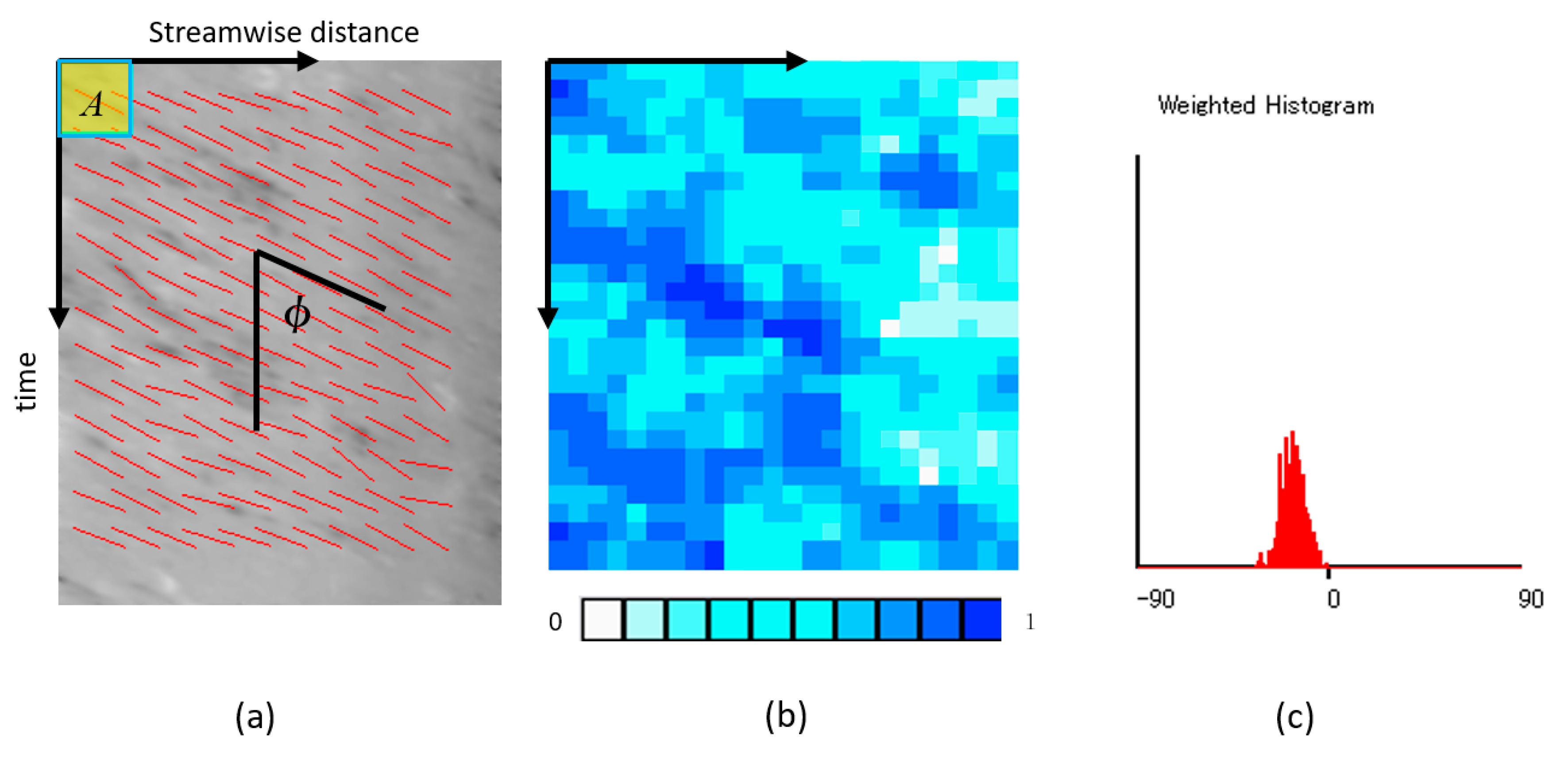
Figure 4.
Water level hydrograph at the measurement site.

Figure 5.
Measurement site description at the Negoya Bridge on the Uono River. L: Panels on the left bank; R: Panels on the right bank; ADCP: acoustic Doppler current profiler; V.M.: velocity meter; FIR: far-infrared-ray; ICHARM: International Centre of Excellence for Water Hazard and Risk Management.

Figure 6.
Comparison of image quality by an FIR camera and a normal high definition video camera: (a) image by FIR camera in the daytime; (b) image by FIR camera at night; (c) image by normal HD camera in the daytime; (d) image by normal HD camera at night.
Figure 6.
Comparison of image quality by an FIR camera and a normal high definition video camera: (a) image by FIR camera in the daytime; (b) image by FIR camera at night; (c) image by normal HD camera in the daytime; (d) image by normal HD camera at night.

Figure 7.
Images from FIR camera A at 10:00: (a) original image taken from the left bank with search lines, (b) ortho-rectified image of (a)
Figure 7.
Images from FIR camera A at 10:00: (a) original image taken from the left bank with search lines, (b) ortho-rectified image of (a)

Figure 8.
Superposed instantaneous velocity vectors measured by large-scale image velocimetry (LSPIV).
Figure 8.
Superposed instantaneous velocity vectors measured by large-scale image velocimetry (LSPIV).

Figure 9.
Space time images obtained by an FIR camera at several transverse locations (units in meters): horizontal scale is 17.6 m and downward vertical scale is ten seconds. Images are enhanced for a better recognition. The dotted line is the main orientation angle of the pattern.
Figure 9.
Space time images obtained by an FIR camera at several transverse locations (units in meters): horizontal scale is 17.6 m and downward vertical scale is ten seconds. Images are enhanced for a better recognition. The dotted line is the main orientation angle of the pattern.
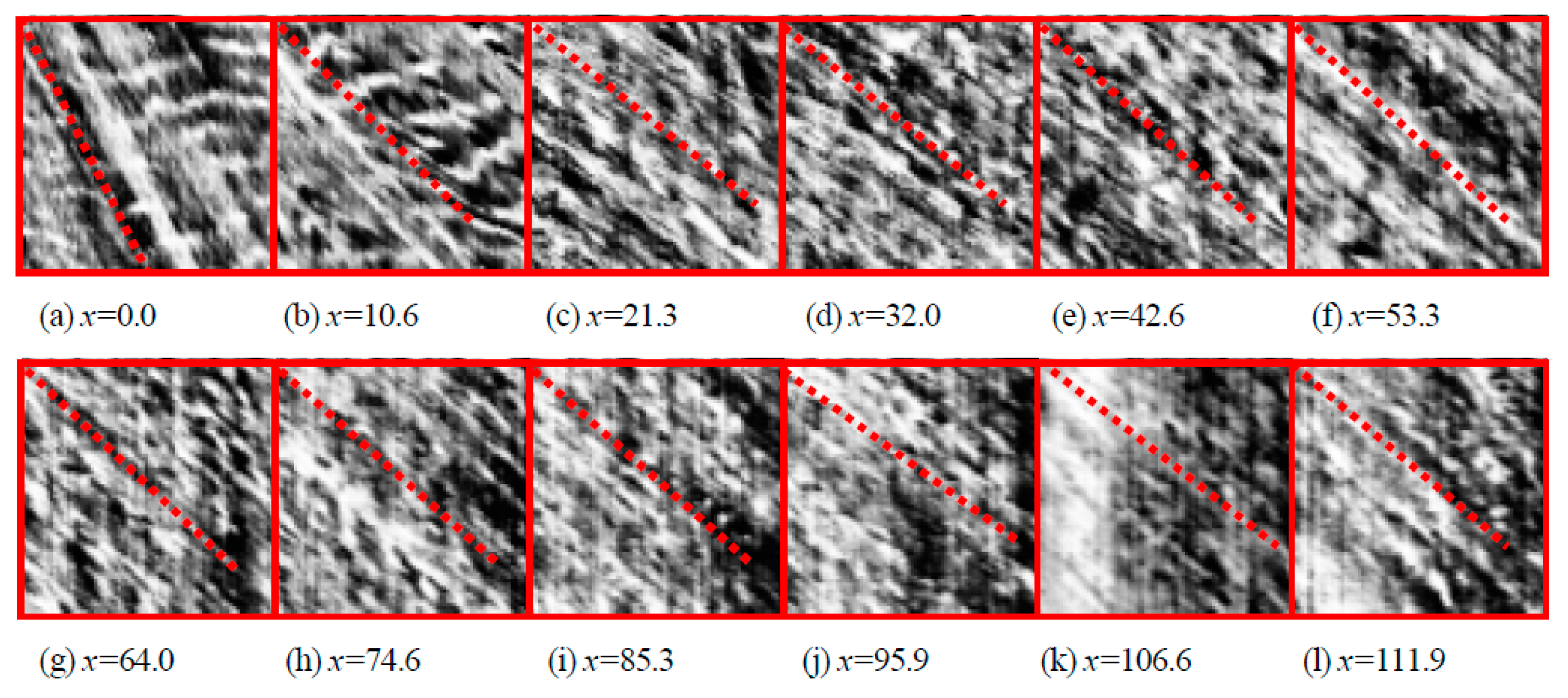
Figure 10.
Comparison of space time image (STI) captured downstream of the bridge in the daytime: (a) STI captured by normal HD camera for a search line along a float trajectory; (b) STI captured by FIR camera for the same search line as (a).
Figure 10.
Comparison of space time image (STI) captured downstream of the bridge in the daytime: (a) STI captured by normal HD camera for a search line along a float trajectory; (b) STI captured by FIR camera for the same search line as (a).
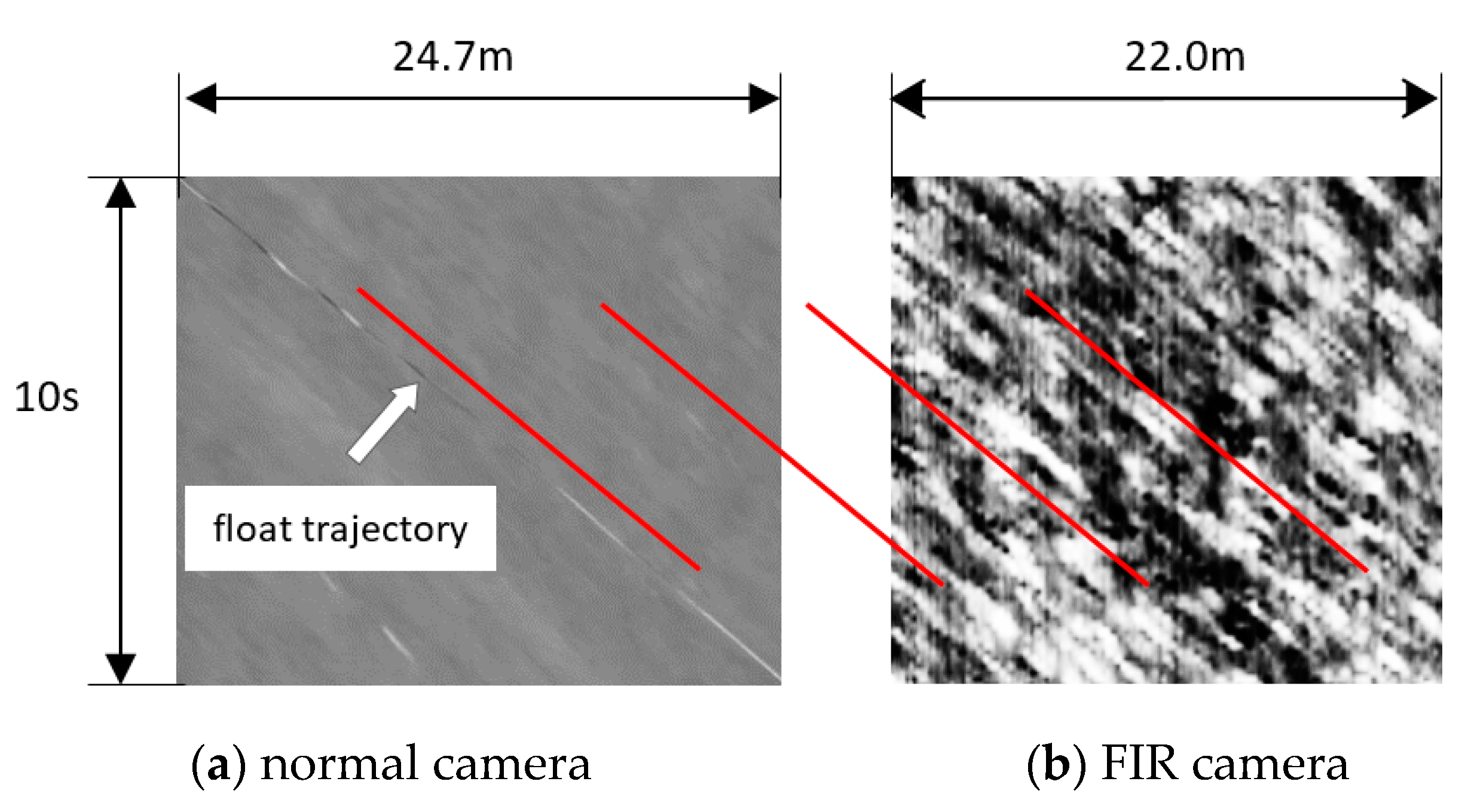
Figure 11.
Comparison of STIs with and without a driftwood obtained at the upstream of the bridge from camera D shown in Figure 5.
Figure 11.
Comparison of STIs with and without a driftwood obtained at the upstream of the bridge from camera D shown in Figure 5.
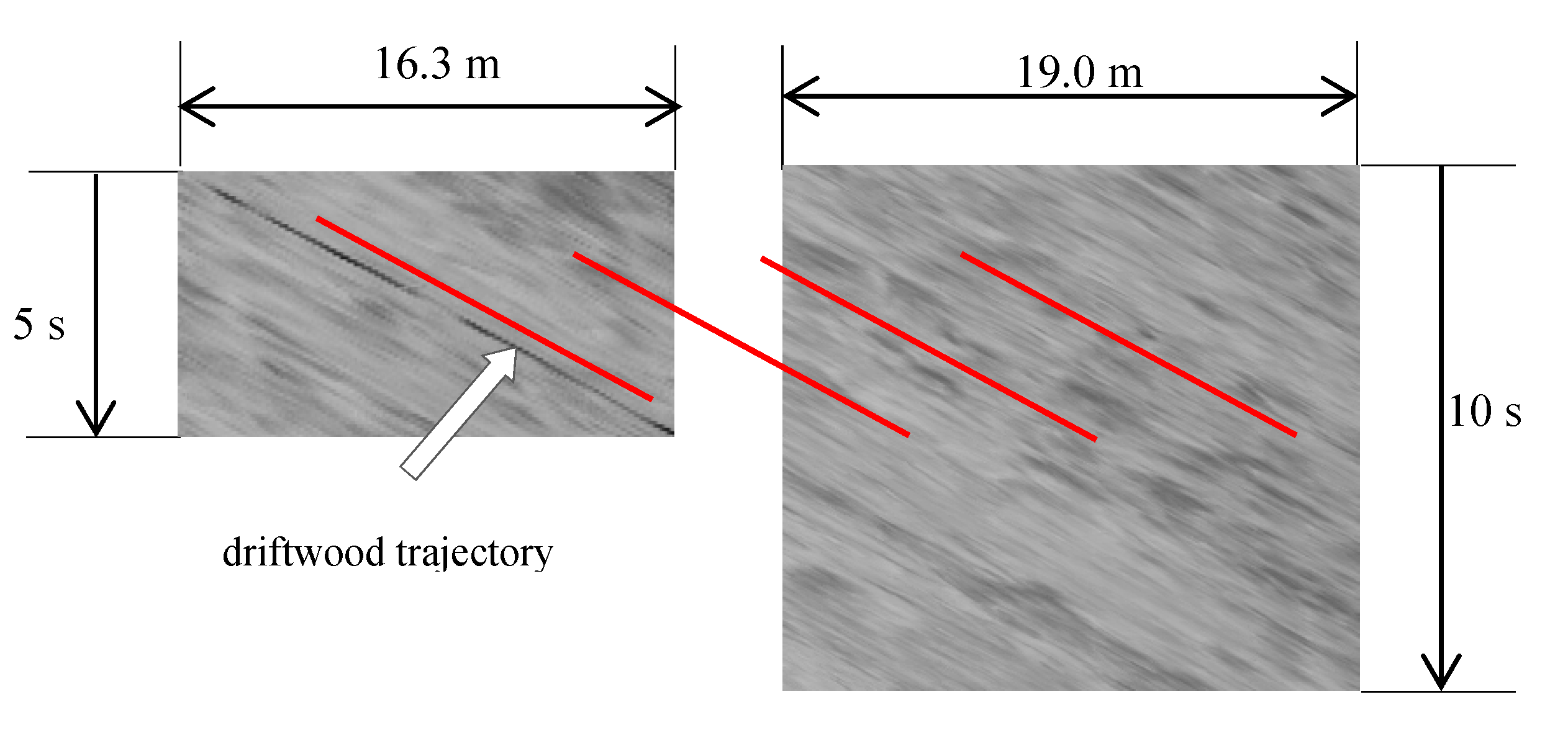
Figure 12.
Comparison of STI obtained at night: (a) STI captured by normal HD camera for a search line along a luminous float trajectory; (b) STI captured by FIR camera for the same search line as (a).
Figure 12.
Comparison of STI obtained at night: (a) STI captured by normal HD camera for a search line along a luminous float trajectory; (b) STI captured by FIR camera for the same search line as (a).

Figure 13.
Comparison of surface velocity distributions by various techniques.
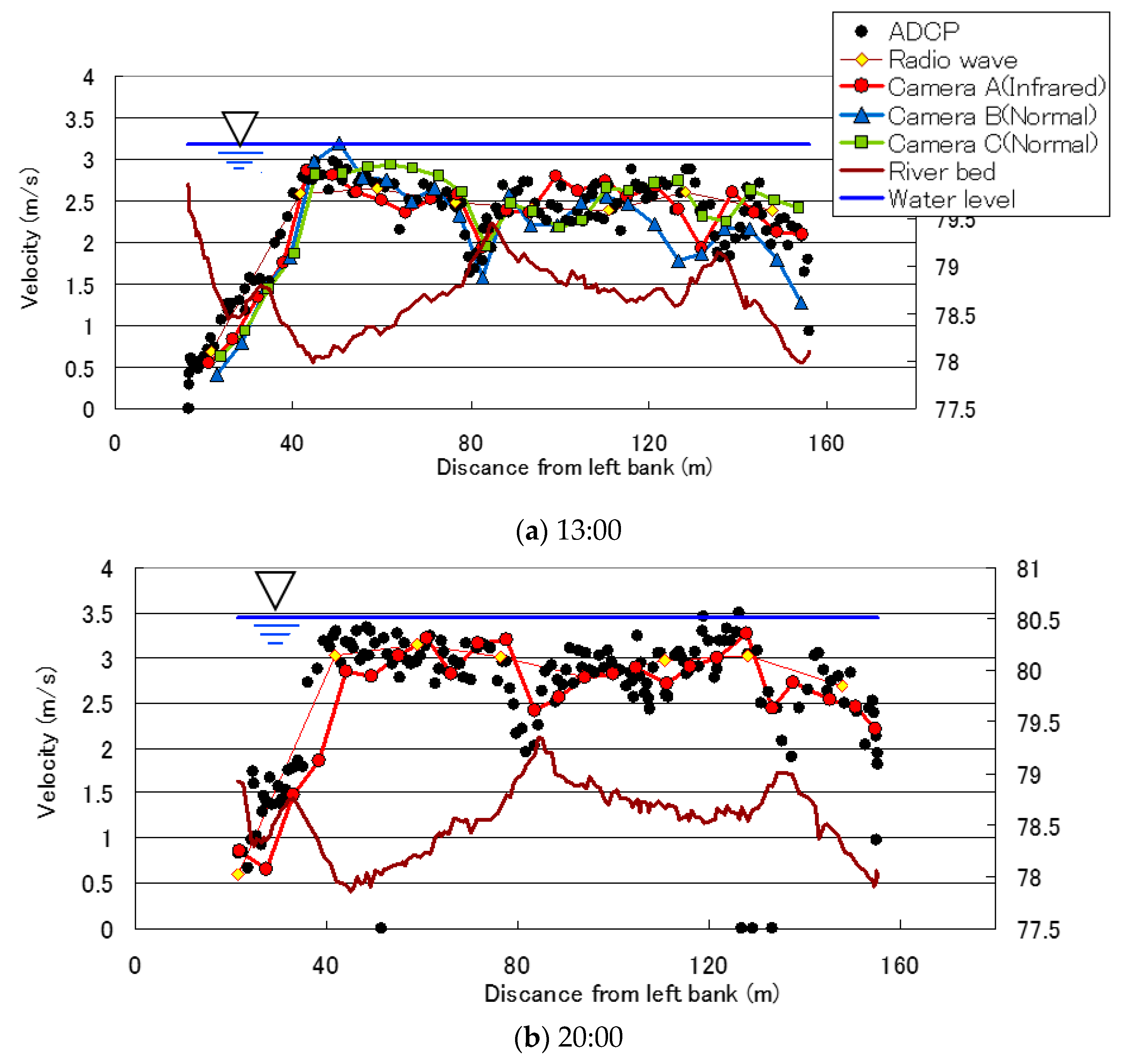
Figure 14.
Surface velocity distribution measured by space time image velocimetry (STIV) at the upstream section of the bridge.
Figure 14.
Surface velocity distribution measured by space time image velocimetry (STIV) at the upstream section of the bridge.
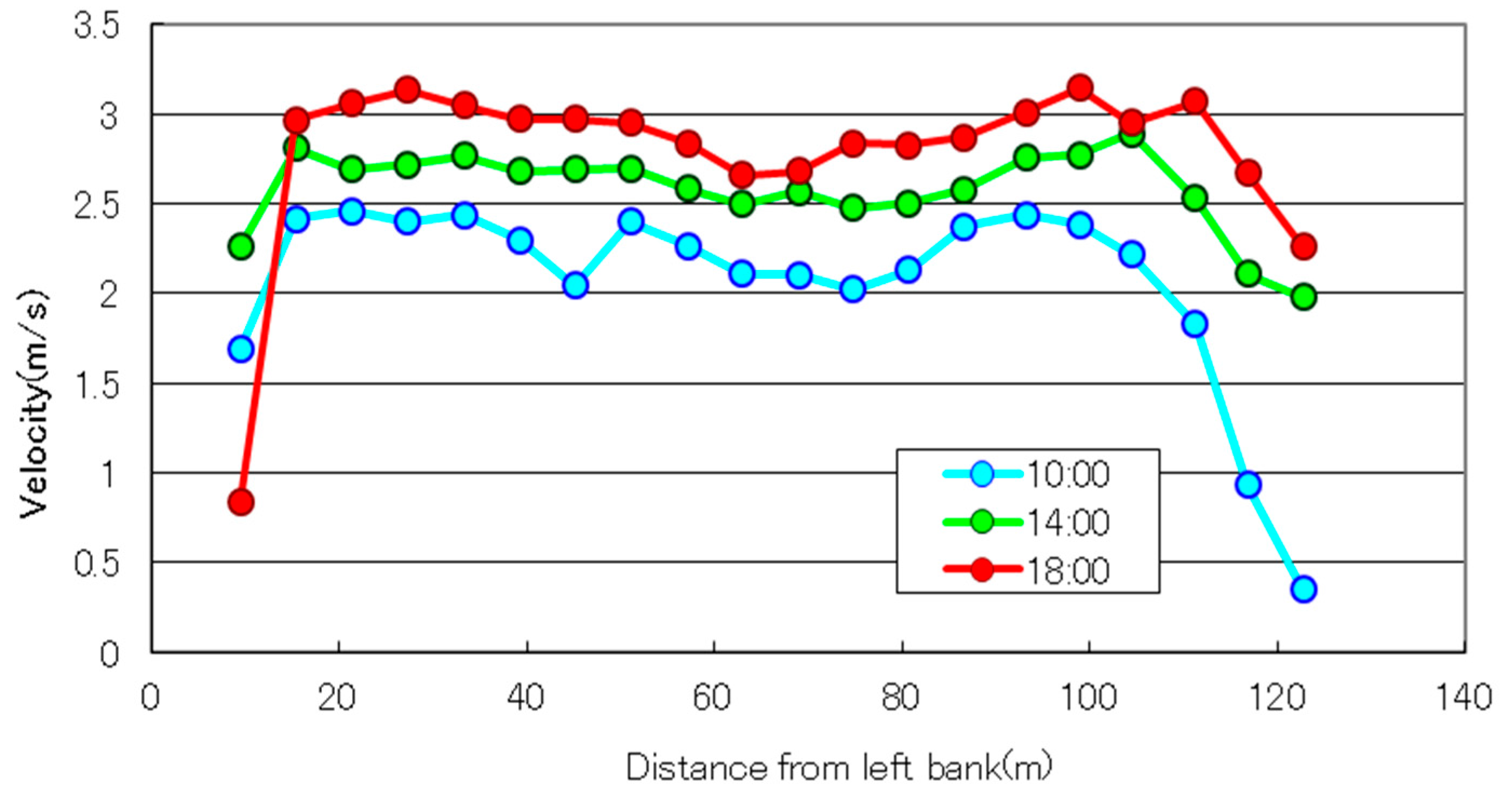
Figure 15.
Comparison of measured discharges.
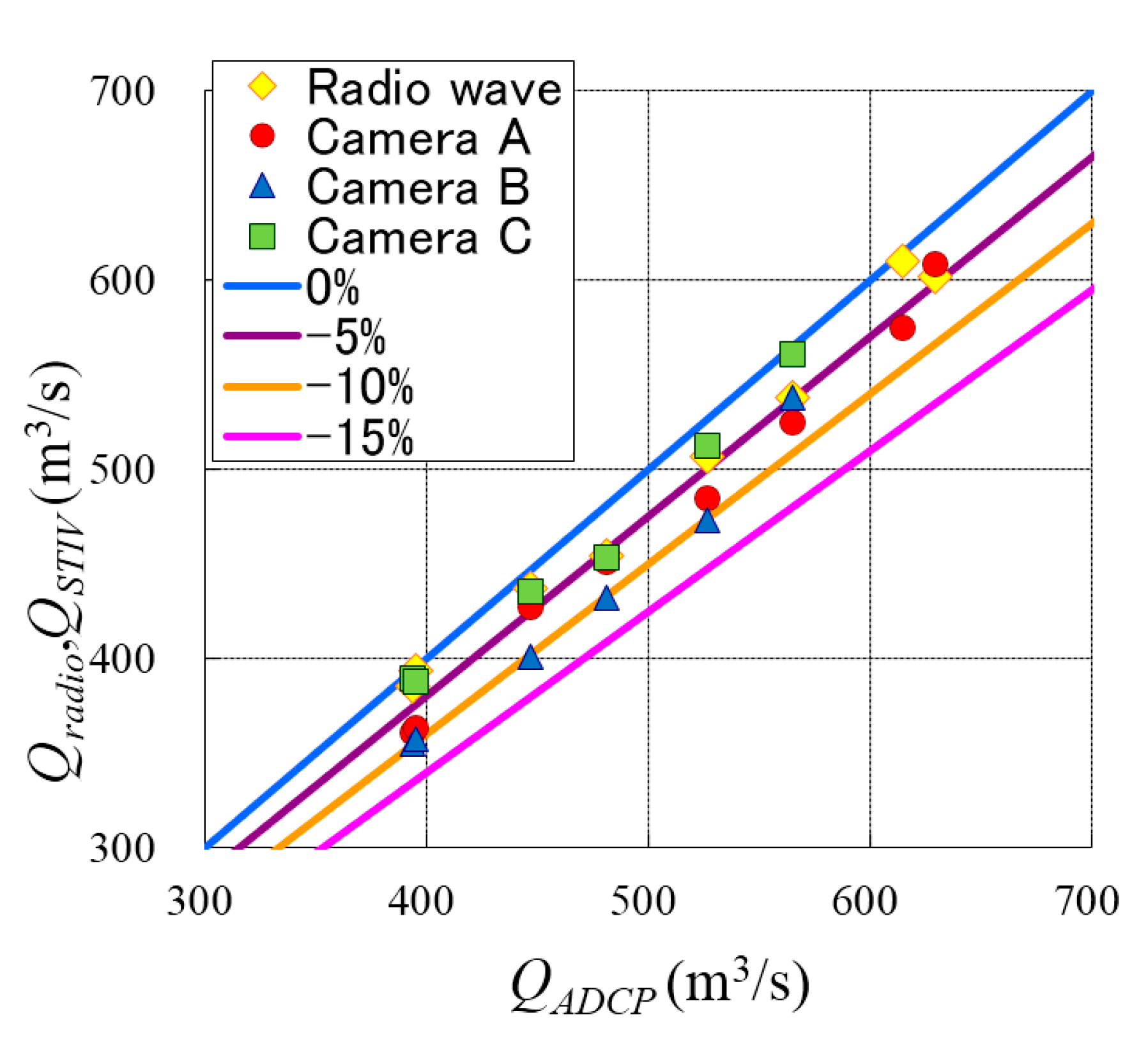
Figure 16.
Discharge hydrographs obtained by various techniques.

© 2017 by the author. Licensee MDPI, Basel, Switzerland. This article is an open access article distributed under the terms and conditions of the Creative Commons Attribution (CC BY) license (http://creativecommons.org/licenses/by/4.0/).
Share and Cite
MDPI and ACS Style
Fujita, I. Discharge Measurements of Snowmelt Flood by Space-Time Image Velocimetry during the Night Using Far-Infrared Camera. Water 2017, 9, 269. https://doi.org/10.3390/w9040269
AMA Style
Fujita I. Discharge Measurements of Snowmelt Flood by Space-Time Image Velocimetry during the Night Using Far-Infrared Camera. Water. 2017; 9(4):269. https://doi.org/10.3390/w9040269
Chicago/Turabian StyleFujita, Ichiro. 2017. "Discharge Measurements of Snowmelt Flood by Space-Time Image Velocimetry during the Night Using Far-Infrared Camera" Water 9, no. 4: 269. https://doi.org/10.3390/w9040269
Note that from the first issue of 2016, this journal uses article numbers instead of page numbers. See further details here.