
Estimation of Active Stream Network Length in a Hilly Headwater Catchment Using Recession Flow Analysis


1
Nanjing Hydraulic Research Institute, Hydrology and Water Resources Department, Nanjing 210029, China
2
Department of Bioproducts and Biosystems Engineering, University of Minnesota, Twin Cities, MN 55108, USA
3
State Key Laboratory of Hydrology-Water Resources and Hydraulic Engineering, and College of Hydrology and Water Resources, Hohai University, Nanjing 210098, China
4
Science and Technology Novelty-Checking Institute, Hohai University, Nanjing 210098, China
*
Authors to whom correspondence should be addressed.
Water 2017, 9(5), 348; https://doi.org/10.3390/w9050348
Submission received: 21 March 2017
/
Revised: 12 May 2017
/
Accepted: 13 May 2017
/
Published: 16 May 2017
(This article belongs to the Special Issue Hillslope and Watershed Hydrology)
Abstract
:Varying active stream network lengths (ASNL) is a common phenomenon, especially in hilly headwater catchment. However, direct observations of ASNL are difficult to perform in mountainous catchments. Regarding the correlation between active stream networks and stream recession flow characteristics, we developed a new method to estimate the ASNL, under different wetness conditions, of a catchment by using streamflow recession analysis as defined by Brutsaert and Nieber in 1977. In our study basin, the Sagehen Creek catchment, we found that aquifer depth is related to a dimensionless parameter defined by Brutsaert in 1994 to represent the characteristic slope magnitude for a catchment. The results show that the estimated ASNL ranges between 9.8 and 43.9 km which is consistent with direct observations of dynamic stream length, ranging from 12.4 to 32.5 km in this catchment. We also found that the variation of catchment parameters between different recession events determines the upper boundary characteristic of recession flow plot on a log–log scale.
1. Introduction
Recession flow analysis has been used to estimate catchment-scale hydraulic parameters for a long time. Brutsaert and Nieber [1] first linked the solution of the Boussinesq equation to a power law relationship as follows:
where Q is discharge during the period of streamflow recession and is the recession rate of discharge. Parameters α and β can be estimated from a −dQ/dt vs. Q plot on a log–log scale. Specifically, α is related to aquifer hydraulic properties by comparing with several analytical solutions of the Boussinesq equation for a horizontal aquifer. Despite some limitations of this method when applied to sloping aquifers [2,3,4], this methodology has subsequently been expanded and applied in many mountainous catchments such as the Yosocuta Watershed in Mexico [5], the Dongjiang Basin in China [6], the arid Coquimbo Region of Chile [7], the Beca River Basin in Portugal [8], and the Massif Central in France [9].
For a given catchment, parameter α in Equation (1) has been found to vary significantly across recession events. It has been shown that aquifer antecedent storage (represented by the average depth of saturated aquifer) has an obvious influence on streamflow recession dynamic and thus on the variation of α [10,11,12,13]. Besides antecedent storage, the dynamic of an active stream network might also lead to the variation of α across recession events. A number of studies have characterized the changes of active stream networks at different spatial and temporal scales. Recently, thorough summaries of this phenomenon were given by Godsey and Kirchner [14] and Shaw [15]. Variances of ASNL have not been widely taken into account in recession flow analysis, although it is a common phenomenon, especially in mountainous catchment. Biswal and Marani [16] proposed that recession flow was a function of the flow per unit of river length and the dynamic stream network, and assumed that recession flow was predominantly controlled by the dynamic stream network in a sloping basin. As a result, the parameters in Equation (1) are related to the signatures of catchment geomorphology [11,17,18,19]. Vannier et al. [9] distinguished the length of permanent and temporary streams in the estimation of catchment-scale soil properties, but did not estimate variation of ASNL across different recession events.
Although whether or not a change of active stream network has a causal effect on the dynamics of streamflow recession is still under debate, there is no doubt that there is a correlation between active stream network and stream recession flow characteristics [14,15,16]. Thus, we propose to estimate ASNL by using an analysis of recession flow. Our study was carried out in Sagehen Creek, a hilly headwater watershed located in the Sierra Nevada mountain range of California.
2. Description of the Study Catchment and Associated Data
Sagehen Creek is located on the east side of the northern Sierra Nevada (Figure 1). The drainage area of the watershed is 27 km2. The land surface elevation in the watershed ranges from 1935 to 2653 m, and the average slope of surface is about 15.8%. The geology of the Sagehen Creek catchment consists of granodiorite bedrock overlain by volcanics, which are overlain by till and alluvium. Although very little is known regarding the depths of different geologic formations, the volcanics are assumed to range in thickness between 50 and 300 m. Alluvium is assumed to range in thickness between 0 and 10 m [20]. Sagehen has a Mediterranean-type climate with cold, wet winters and warm, dry summers [21]. Mean annual temperature from 1980 to 2002 was 4 °C, at an altitude of 2545 m. Mean annual precipitation from 1960 to 1991 was 970 mm. Approximately 80% of precipitation falls as snow. Daily mean streamflow data were obtained at the gage near the outlet of the catchment (gauging station number: 10343500). Mean daily streamflow was approximately 1 m3/s during snowmelt in May and June for 1953–2003. Sagehen Creek is a documented example of the application of the GSFLOW model to a watershed [20]. The GSFLOW model is composed of a surface water model—PRMS—coupled with MODFLOW, a groundwater flow model [20]. In the Markstrom et al. study [20], the GSFLOW model was calibrated to simulate the observed streamflow given the observed meteorological data collected for Sagehen Creek watershed. The calibrated hydraulic conductivity and specific yield for the alluvium have ranges of 0.026–0.39 m/d and 0.08–0.15, respectively. The geometric means of hydraulic conductivity and specific yield are 0.075 m/d and 0.1, respectively. A period of 16 water years, 1 October 1980 to 30 September 1996 was taken in this research. This time period was previously evaluated by the GSFLOW model. As such, recession flow analysis can be performed by using more reliable hydrologic fluxes (infiltration, actual evapotranspiration) simulated by GSFLOW. Digital elevation model data, at 30 m resolution, were obtained from USGS (available at: http://nationalmap.gov/viewer.html) and were used to stream network analysis in Section 3.2.
3. Method
3.1. Theory
One of the most commonly used analytical solutions for discharge recession of sloping aquifers was formulated by Brutsaert [22]. This solution gives the outflow from the hillslope as
where Q is the discharge out of the aquifer, , , p is a constant assumed to be 0.3465 [1,2,23], is the slope angle of the aquifer, k is the hydraulic conductivity, f is the specific yield, B is the active stream network length, D is the initial saturated thickness of the aquifer, L is the breadth of the aquifer, and is the th root of Equation (3), which can be computed numerically with
In the case where in Equation (2), the discharge (Q) from the aquifer is simplified to
Then the recession rate of the discharge can be written as
Thus
As was shown by Rupp and Selker [2] and Pauritsch et al. [4], when dQ/dt and Q derived from Equation (2) are plotted on a log–log scale, the recession curve has an obvious transition point, which separates the curve into an early time domain and a late time domain. The curve in the early time domain is concave. A similar concave recession pattern was also found based on observed streamflow in Sagehen Creek (shown later in Section 3.3). We consider the early time domain to be the more typical case, at least in Sagehen Creek, because in many cases rainfall events prevent recessions from extending beyond the early time period. Since the short time behavior illustrated by Equations (4)–(7) should be the initial segment of early time domain, we used Equation (6) and the early time solution of Equation (2) to perform the following parameter estimation.
3.2. Estimation of Aquifer Breadth
In general, the breadth of the aquifer is calculated as
where A is the catchment area. When we treat the stream network length as a dynamic rather than a stable variable, the area also should be taken as the contribution area related to the active stream instead of the total area. Otherwise, Equation (8) will lead to an unrealistically large value of L when ASNL shrinks significantly.
Based on the empirically observed dynamic of the stream network [24], the hillslopes including order-one streams stop contributing to streamflow first, indicating the shrinkage of the contribution area. As the catchment drainage continues, only the areas connected to high order streams contribute. Following this general idea as shown in Figure 1, we used GIS to generate a stream network with a total length of 30.6 km, including three Strahler orders by ignoring several minor details. A total of 16 first-order tributaries with the combined length of 20.8 km were found (dashed lines in Figure 1). Each of them relates to a hillslope contribution area (the gray zone in Figure 1). With the assumption that the hillslope will stop contributing to higher order stream as soon as the related order-one tributary shrinks totally, we generated a series of ASNL and contributing areas with different combinations of the shrinkage of order-one streams. Figure 2 shows the calculated breadth based on Equation (8), with the dynamic contributing area and ASNL. As a result of our calculations, the breadth has a narrow range, from 413 m to 517 m, with a mean of 452 m and a standard deviation of 16.2 m. This illustrates that the breadth has a relatively stable value with the variation of the active stream network. This is not surprising, since the breadth of the aquifer is a transformation of drainage density, which tends to reach a state of equilibrium [25,26].
3.3. Recession Flow Analysis
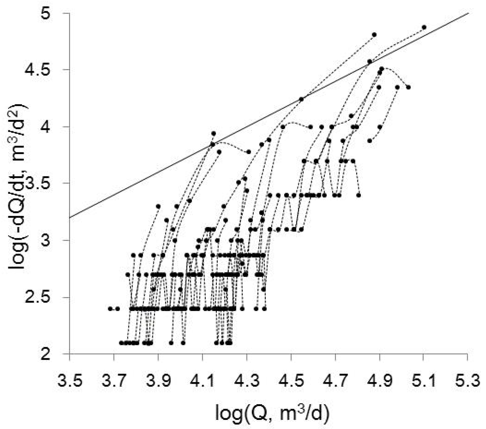
Recession analysis was carried out based on the observed streamflow over the 16-year period. The backward difference approximation of dQ/dt (=(Qt−△t − Qt)/△t) was calculated using consecutive daily flows and plotted against the arithmetic mean ((Qt−△t + Qt)/2) of the corresponding flows [1]. Next, along with simulated actual daily evapotranspiration (AET) from the soil, and infiltration (AI) into the soil—both calculated by the GSFLOW model—recession stream flows were selected according to the following criteria [27,28,29]: (1) data points with no positive values of dQ/dt, and (2) data points when the absolute ratio of (AI-AET) to observed Q is smaller than 0.1. As a result, 51 individual recessions with at least four continuous days’ length were derived. As is shown in Figure 3, the plot of these individual recessions produces a concave shape.
Two details should be considered when applying these selected recession curves. One is the influence of snowmelt. Snowmelt water can exceed the infiltration capacity of the soil, and GSFLOW does calculate the infiltration and surface runoff generated by snowmelt. Since the selection of recession data was based on the absences of significant net infiltration (AI-AET) during the recession period, we assumed there was no significant snowmelt during the selected recessions. Thus, the influence of snowmelt may be ignored, although minor snowmelt may discharge to the stream directly. The second important detail is the inverse U shape of several recession curves at the beginning of the recession. Consistent with Pauwels and Troch [30], the inverse U shape can be explained by the effect of recharge. The (AI-AET) metric calculated by the GSFLOW model was not completely consistent with the infiltration in the real catchment, although the model has been calibrated. Hence the recessions derived from the observed streamflow still can be influenced by real recharge. These initial data points were ignored during the following analysis.
3.4. Estimation of ASNL
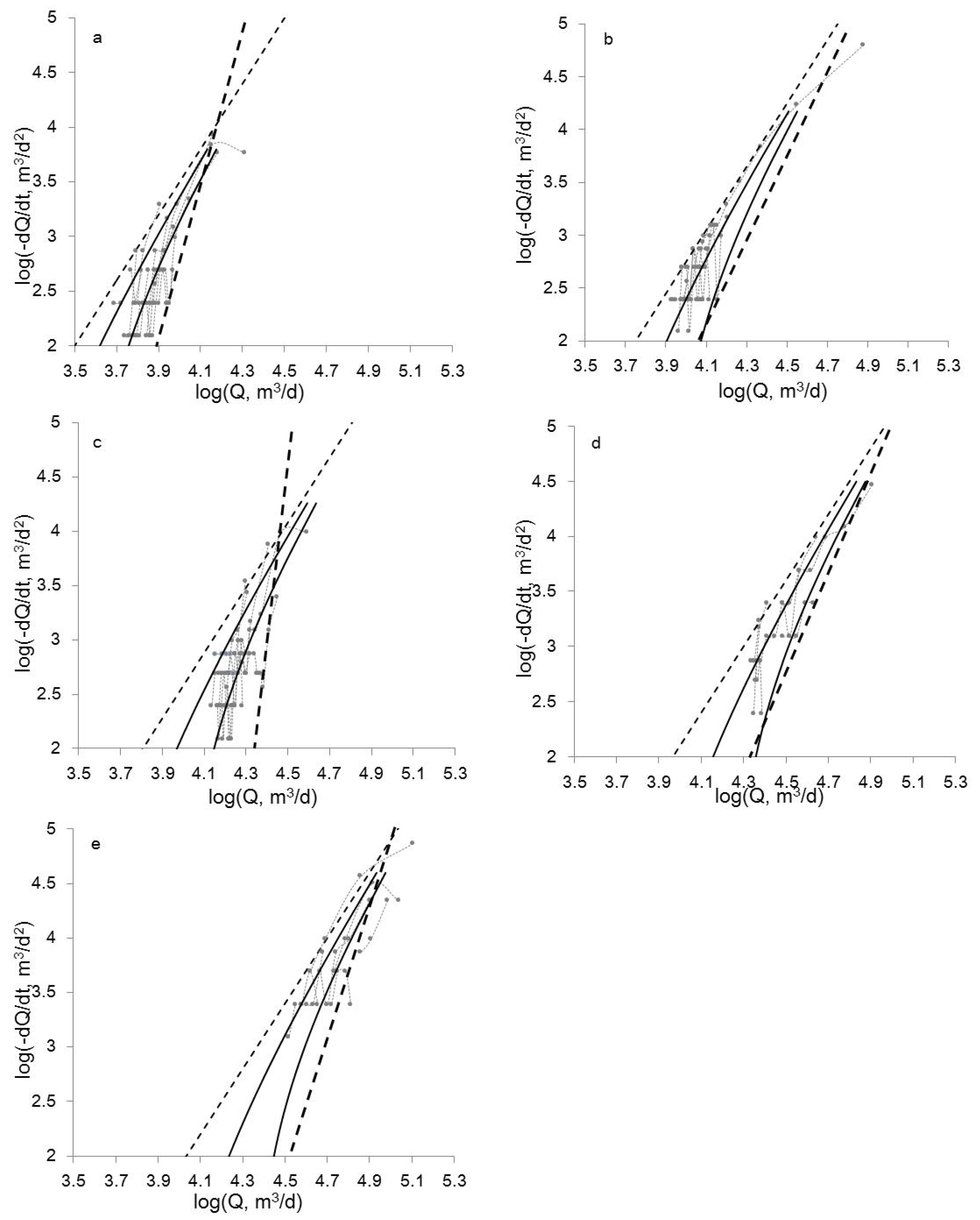
The 51 individual recession curves were separated into several ranges according to the logarithmic values of the minimum discharge at the end of each recession (Qmin). The number of ranges was chosen subjectively to make each range include at least seven recession curves with similar values of Qmin. As a result, five ranges were used, and are shown in Figure 4 and Table 1. The mean discharge of recessions of each range varies between 8054–58,899 m3/d and encompasses a wide range of wetness conditions. Each plot in Figure 4 was indicated by two straight dash lines. The upper envelope was placed with a slope of 3. In keeping with Equation (5), this upper envelope represented the short time recession behavior. The lower envelope was placed visually by ignoring the data points with an inverse U shape. Thus, all of these initial data points were ignored during the following analysis.
The value of log (α) is taken as the intercept of the line of upper envelope with y-axis. Key values of each plot are summarized in Table 1. With the geometric means of k and f, and the mean of L estimated in Section 3.2, B can be obtained using Equation (6) as long as D is specified, and then the recession flow is calculated with Equation (2). The calculation process was repeated by increasing D from 0 with an interval of 1 m regularly. Only the values of D which led to the recession curve (dQ/dt vs. Q on a log–log scale) being located between two envelopes in Figure 4 were noted down. Hence the ranges of both D and B were obtained.
4. Results
As a result, the preliminary range of D, 4–27 m, was estimated, which is not related to α. The two black curves shown in Figure 4 are based on the solutions of Equation (2) when D equals 4 m (right curve), and 27 m (left curve). We infer that the established range of D is only related to a dimensionless parameter, , which represents the magnitude of the slope term in Equation (2) [22]. When D is large enough (more than 27 m in this case), −aL has a small value, which leads to the catchment’s behavior as a horizontal flow. Under this condition, the concave shape of the early recession curve disappears. On the other hand, for a small value of D (less than 4 m in this case), −aL is large, which lead the catchment to behave as a steeper aquifer. In this case, the duration of early recession is very short, less than one day; it therefore cannot be shown in a log–log plot with a time interval of one day.
In fact, Equation (6) illustrates a negative power law relationship between B and D. Figure 5 shows the curves of B vs. D for all of the five different ranges illustrated by Figure 4. The range of ASNL estimated by Equation (6) is shown in Table 1. Thus, a maximum range of stream network length, 1.6–173.5 km, can be obtained. With several additional assumptions, a more reasonable range of ASNL might be concluded. For example, as stated in Section 2, the thickness of alluvium in Sagehen Creek catchment is assumed to range between 0 and 10 m. If we take the saturated aquifer depth as 10 m in the wettest conditions (illustrated by curve e in Figure 5), ASNL would be estimated at 43.9 km. It is reasonable to expect the shrinkage of the stream network and decrease of the saturated aquifer’s depth during the drying period of the catchment. The reasonable range of ASNL should thus be located in the gray zone shown in Figure 5. Moreover, with the assumption that only stream channels with high orders are active in dry conditions (illustrated by curve a in Figure 5), ASNL is expected to equal the length of the high order stream based on the result in Section 3.2, which is 9.8 km. As a result, the estimated ASNL is between 9.8 km and 43.9 km. With the illustrated dash line in Figure 5, each value of ASNL related to five different ranges can be further estimated. The results are shown in Table 1.
5. Discussion
5.1. Comparison with Prior Results
Godsey and Kirchner [14] calculated dynamic stream length based on a field survey in Sagehen Creek. They found the connected flowing network length had a range of 12.4–32.5 km. while the stream flow discharge had a range of 4080–47,872 m3/d. Consistent with their results, we revealed a range of 9.8–43.9 km when the average stream flow discharge ranges between 8054–58,899 m3/d. Another estimation can be obtained from The National Hydrography Dataset (NHD) (http://nhd.usgs.gov/) maps. The NHD was developed by the USGS to support hydrography research [31]. Based on the NHD of Sagehen Creek, we calculated the lengths of the perennial, intermittent, and ephemeral stream, which are 6.8, 3.7, and 62.4 km respectively. The total stream network length is 72.9 km, which is about twice the estimated ASNL in wet conditions found in our research. One possibility for the discrepancy is that the length of stream in the NHD was mapped in high resolution (The map scale of the high-resolution NHD is 1:24,000), so that some minor channels were also mapped. These minor channels are mostly active only during rainfall events and transit surface runoff. We estimated ASNL based only on the recession flow discharging mostly from catchment storage, and ignored the influence of the surface runoff. Thus the minor stream network should shrink, and was not taken into account in our research. Another possibility is that the saturated depth in wet conditions may be smaller than 10 m. For example, when the saturated depth is taken as 7 m in wet conditions, a channel length of 74.9 km can be estimated based on the curve in Figure 5. However, without more detailed information on the dynamics of the groundwater table for Sagehen Creek, it is not easy to quantify the saturated depth accurately.
5.2. Uncertainty of the Parameters
As stated in Section 3.1, the analytical solution for an ideal rectangle sloping aquifer was used to perform the estimation of ASNL. It is obvious that a real catchment, such as Sagehen Creek, is far more complicated than a simple ideal catchment. Thus the catchment(s) average parameters, such as i, D, k, f, etc., should be obtained using an appropriate method. To account for the spatial variability of the catchment properties, these parameters are usually calculated with a reasonable range instead of a unique value. Thus, the uncertainty of the parameters in Equations (2)–(6) will introduce inaccuracy to the result. As shown in Section 5.1, the estimated ASNL changes significantly when the saturated depth value changes.
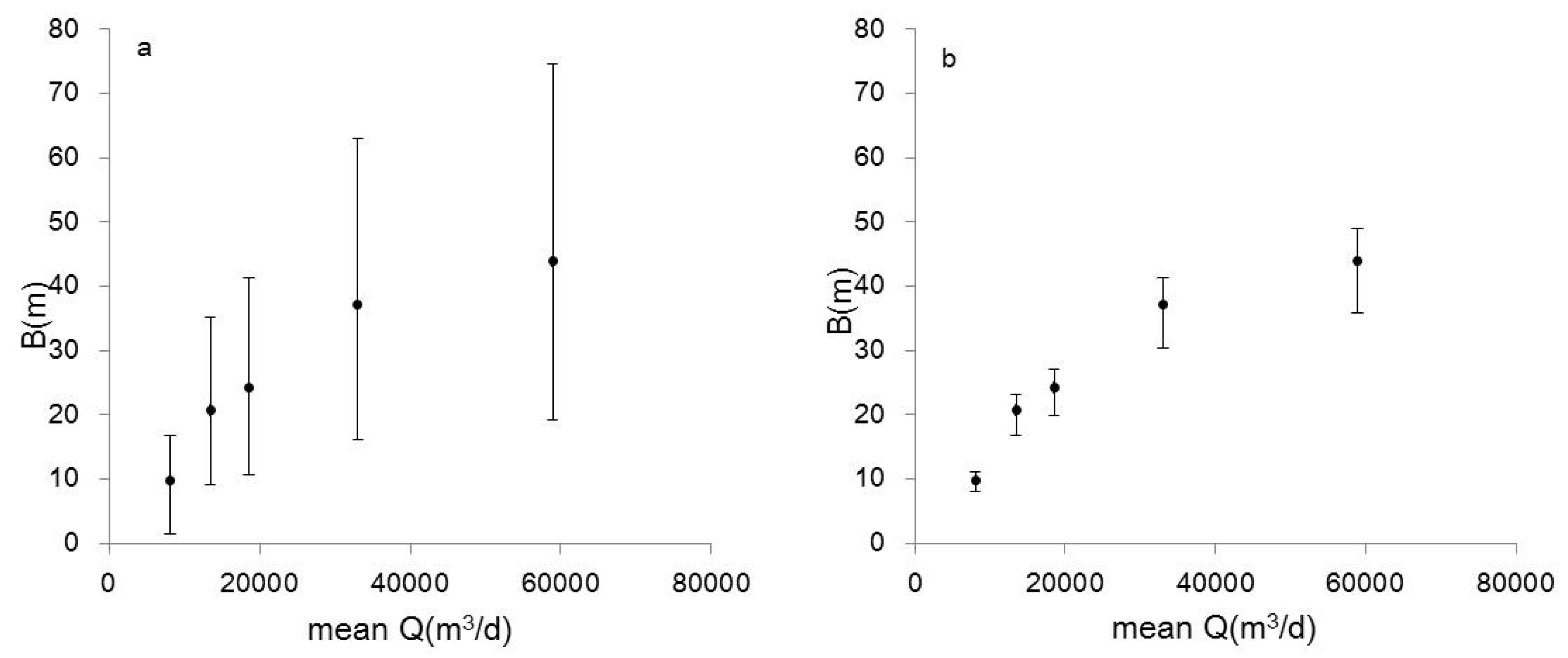
To reveal the influence of parameter uncertainty on the estimated result, sensitivity analysis of k and f was further carried out. Based on the parameters calibration result using GSFLOW in Sagehen Creek, the analysis range of k and f was taken as 0.026–0.39 m/d and 0.08–0.15, respectively. As in shown in Figure 6, the sensitivity of the results to f seems relatively limited, while the variation of k has obvious influence on the estimated results. The method proposed by Brutsaert and Nieber [1] is focused on the estimation of catchment averaged hydrogeological properties; thus, we consider the geometric means of k and f to be more appropriate in use as input for the estimation than their maximum or minimum values.
Consistent with prior research, and inherent to our research, is the assumption that there is no change in k and f in different recession events for a given catchment. As shown in Table 1, α increases by almost 40 times from wet to dry conditions. This would also imply the significant decrease of the product (kf), based on the negative relationship between α and kf shown by Equation (6). However this is less realistic. When the catchment dries and saturated areas shrink, the hydraulic response is dominated by riparian areas [32], and thus both k and f should increase generally. As a result, the most probable reason for the increase of α is the shrinking of ASNL when the watershed dries up.
5.3. Advantages and Limitations
The presented approach shows how to estimate ASNL by using recession flow analysis. This research moves our knowledge of recession flow forward. That is, the information embedded in observed recession streamflows can be used not only to estimate hydrogeology parameters, but also to estimate the total length of an active stream, especially in a hilly catchment. The method mainly relies on measured streamflow at the outlet of the catchment, thus it can be easily applied to other catchments.
However, the limitations are also obvious. Since we used observed streamflow at the gauge of catchment outlet, only those active stream channels connecting to the outlet can be estimated. Godsey and Kirchner [14] showed many disconnected stream channels based on their field survey. These disconnected stream channels cannot be estimated by the present approach. Another limitation of this study is that only one hilly catchment, Sagehen Creek, was tested. The accuracy of the method may be influenced by the catchment characteristics, such as topography, geology, climate etc. For example, the stream network would likely be less dynamic in a flat and rainy catchment, so that ASNL may be taken as static instead of dynamic and recession flow characteristics should have less relationship to channel length. More complete and reliable conclusions about the present approach will be reached only after broad applications in different catchments.
5.4. Precautions and Requirements
In this study, net infiltration flux (AI-AET) calculated by GSFLOW was used to select recession stream flows. Hydrologic fluxes are generally not known, but would be determined from measurements or calculated using some acceptable method. Thus, before the application of the present approach to a given catchment, hydrologic fluxes such as actual evapotranspiration and infiltration should be estimated based on some other method a priori. It is also necessary to have some preliminary understanding of catchment parameters such as hydraulic conductivity, specific yield, aquifer thickness, and slope angle of the aquifer. Generally, the more accurate these parameters are, the less the uncertainty of the estimated ASNL.
5.5. The Behavior of Short Time Recession
As shown in Figure 3, a cloud of −dQ/dt vs. Q points is composed of a bunch of recession curves. The upper boundary of these points illustrates short time recession flow behavior between different recession events. An upper boundary with a slope of 1 has also been observed in other studies [5,7,8,33,34]. While it has not been discussed widely, Mendoza et al. [5] hypothesized that this 1:1 line might represent some maximum physical limit of the contributing aquifer on otherwise random-like recession flow behavior. We infer that this upper boundary with a slope of 1 reflects the variation of catchment parameters between different recession events. Based on Equations (4) and (6), the log form of Q and dQ/dt can be shown as
Thus
As in shown by Equations (9) and (10), although the change of certain parameters (B, k, f, D, or i) between different recession events would lead to variations of α and the shape of recession curves, the variation of α has an equivalent influence on the magnitudes of Q and dQ/dt in a log–log scale. That is, as indicated by Equation (11), those data points with the same recession time (t) between different recession events would be located on a straight line with a slope of 1 and a y-intercept of −log(2t). It should be noted that this behavior is reflected only by the very early recession data, since Equations (4) and (6) are only valid for short recession times.
6. Concluding Remarks
Varying ASNL is a common phenomenon, especially in hilly headwater catchments. Accurate estimation of ASNL is valuable for hydrological modeling and is essential to hydro ecosystem maintenance and water resource sustainability. To address the difficulty in direct measurement of changes in the active stream network, this research links ASNL to recession flow dynamic. This approach shows how to estimate ASNL by using analysis of recession flow. To our knowledge, this has never been carried out before. In this first application to the Sagehen Creek catchment, the estimated range of ASNL is consistent with prior results. More complete and reliable conclusions about the present approach will be reached after broad applications in different catchments.
Acknowledgments
This research was partially supported by National Key Research and Development Program of China (No. 2016YFC040281002, 2016YFC0402808, and 2016YFC0402701), National Nature Science Foundation of China (No. 51409161), Natural Science Foundation of Jiangsu Province (Grants No. BK20140080), the Fundamental Research Funds for the Central Universities of China (No. 2015B28514), and the Priority Academic Program Development of Jiangsu Higher Education Institutions.
Author Contributions
Wei Li served as lead and corresponding author, and designed the program of research; Ke Zhang performed the analyses; Yuqiao Long provided editorial improvements to the paper; Li Feng analyzed the background of recession flow and improved the introduction.
Conflicts of Interest
The authors declare no conflict of interest.
References
- Brutsaert, W.; Nieber, J.L. Regionalized Drought Flow Hydrographs from a Mature Glaciated Plateau. Water Resour. Res. 1977, 13, 637–643. [Google Scholar] [CrossRef]
- Rupp, D.E.; Selker, J.S. On the use of the Boussinesq equation for interpreting recession hydrographs from sloping aquifers. Water Resour. Res. 2006, 42. [Google Scholar] [CrossRef]
- Bogaart, P.W.; Rupp, D.E.; Selker, J.S.; van der Velde, Y. Late-time drainage from a sloping Boussinesq aquifer. Water Resour. Res. 2013, 49, 7498–7507. [Google Scholar] [CrossRef]
- Pauritsch, M.; Birk, S.; Wagner, T.; Hergarten, S.; Winkler, G. Analytical approximations of discharge recessions for steeply sloping aquifers in alpine catchments. Water Resour. Res. 2015, 51, 8729–8740. [Google Scholar] [CrossRef]
- Mendoza, G.F.; Steenhuis, T.S.; Walter, M.T.; Parlange, J.-Y. Estimating basin-wide hydraulic parameters of a semi-arid mountainous watershed by recession-flow analysis. J. Hydrol. 2003, 279, 57–69. [Google Scholar] [CrossRef]
- Zhang, L.; Chen, Y.D.; Hickel, K.; Shao, Q. Analysis of low-flow characteristics for catchments in Dongjiang Basin, China. Hydrogeol. J. 2008, 17, 631–640. [Google Scholar] [CrossRef]
- Oyarzún, R.; Godoy, R.; Núñez, J.; Fairley, J.P.; Oyarzún, J.; Maturana, H.; Freixas, G. Recession flow analysis as a suitable tool for hydrogeological parameter determination in steep, arid basins. J. Arid Environ. 2014, 105, 1–11. [Google Scholar] [CrossRef]
- Santos, R.M.B.; Sanches Fernandes, L.F.; Moura, J.P.; Pereira, M.G.; Pachecoe, F.A.L. The impact of climate change, human interference, scale and modeling uncertainties on the estimation of aquifer properties and river flow components. J. Hydrol. 2014, 519, 1297–1314. [Google Scholar] [CrossRef]
- Vannier, O.; Braud, I.; Anquetin, S. Regional estimation of catchment-scale soil properties by means of streamflow recession analysis for use in distributed hydrological models. Hydrol. Process. 2014, 28, 6276–6291. [Google Scholar] [CrossRef]
- Bart, R.; Hope, A. Inter-seasonal variability in baseflow recession rates: The role of aquifer antecedent storage in central California watersheds. J. Hydrol. 2014, 519, 205–213. [Google Scholar] [CrossRef]
- Biswal, B.; Nagesh Kumar, D. Study of dynamic behaviour of recession curves. Hydrol. Process. 2014, 28, 784–792. [Google Scholar] [CrossRef]
- Patnaik, S.; Biswal, B.; Nagesh Kumar, D.; Sivakumaer, B. Effect of catchment characteristics on the relationship between past discharge and the power law recession coefficient. J. Hydrol. 2015, 528, 321–328. [Google Scholar] [CrossRef]
- Shaw, S.B.; McHardy, T.M.; Riha, S.J. Evaluating the influence of watershed moisture storage on variations in base flow recession rates during prolonged rain-free periods in medium-sized catchments in New York and Illinois, USA. Water Resour. Res. 2013, 49, 6022–6028. [Google Scholar] [CrossRef]
- Godsey, S.E.; Kirchner, J.W. Dynamic, discontinuous stream networks: Hydrologically driven variations in active drainage density, flowing channels and stream order. Hydrol. Process. 2014, 28, 5791–5803. [Google Scholar] [CrossRef]
- Shaw, S.B. Investigating the linkage between streamflow recession rates and channel network contraction in a mesoscale catchment in New York state. Hydrol. Process. 2016, 30, 479–492. [Google Scholar] [CrossRef]
- Biswal, B.; Marani, M. Geomorphological origin of recession curves. Geophys. Res. Lett. 2010, 37, L24403. [Google Scholar] [CrossRef]
- Mutzner, R.; Bertuzzo, E.; Tarolli, P.; Weijs, S.V.; Nicotina, L.; Ceola, S.; Tomasic, N.; Rodriguez-Iturbe, I.; Parlange, M.B.; Rinaldo, A. Geomorphic signatures on Brutsaert base flow recession analysis. Water Resour. Res. 2013, 49, 5462–5472. [Google Scholar] [CrossRef]
- Biswal, B.; Nagesh Kumar, D. What mainly controls recession flows in river basins? Adv. Water Resour. 2014, 65, 25–33. [Google Scholar] [CrossRef]
- Biswal, B.; Marani, M. ‘Universal’ recession curves and their geomorphological interpretation. Adv. Water Resour. 2014, 65, 34–42. [Google Scholar] [CrossRef]
- Markstrom, S.L.; Niswonger, R.G.; Regan, R.S.; Prudic, D.E.; Barlow, P.M. GSFLOW-Coupled Ground-Water and Surface-Water FLOW Model Based on the Integration of the Precipitation-Runoff Modeling System (PRMS) and the Modular Ground-Water Flow Model (MODFLOW-2005); U.S. Geological Survey: Reston, VA, USA, 2008; p. 240.
- Manning, A.H.; Clark, J.F.; Diaz, S.H.; Rademacher, L.K.; Earman, S.; Plummer, L.N. Evolution of groundwater age in a mountain watershed over a period of thirteen years. J. Hydrol. 2012, 460–461, 13–28. [Google Scholar] [CrossRef]
- Brutsaert, W. The unit response of groundwater outflow from a hillslope. Water Resour. Res. 1994, 30, 2759–2763. [Google Scholar] [CrossRef]
- Brutsaert, W.; Lopez, J.P. Basin-scale geohydrologic drought flow features of riparian aquifers in the Southern Great Plains. Water Resour. Res. 1998, 34, 233–240. [Google Scholar] [CrossRef]
- Chen, B.; Krajewski, W.F. Recession analysis across scales: The impact of both random and nonrandom spatial variability on aggregated hydrologic response. J. Hydrol. 2015, 523, 97–106. [Google Scholar] [CrossRef]
- Brutsaert, W. Long-term groundwater storage trends estimated from streamflow records: Climatic perspective. Water Resour. Res. 2008, 44. [Google Scholar] [CrossRef]
- Lyon, S.W.; Giesler, R.; Humborg, C. Estimation of permafrost thawing rates in a sub-arctic catchment using recession flow analysis. Hydrol. Earth Syst. Sci. 2009, 13, 595–604. [Google Scholar] [CrossRef]
- Kirchner, J.W. Catchments as simple dynamical systems: Catchment characterization, rainfall-runoff modeling, and doing hydrology backward. Water Resour. Res. 2009, 45. [Google Scholar] [CrossRef]
- Stoelzle, M.; Stahl, K.; Weiler, M. Are streamflow recession characteristics really characteristic? Hydrol. Earth Syst. Sci. 2013, 17, 817–828. [Google Scholar] [CrossRef]
- Shaw, S.B.; Riha, S.J. Examining individual recession events instead of a data cloud: Using a modified interpretation of dQ/dt–Q streamflow recession in glaciated watersheds to better inform models of low flow. J. Hydrol. 2012, 434–435, 46–54. [Google Scholar] [CrossRef]
- Pauwels, V.R.N.; Troch, P.A. Estimation of aquifer lower layer hydraulic conductivity values through base flow hydrograph rising limb analysis. Water Resour. Res. 2010, 46. [Google Scholar] [CrossRef]
- Simley, J.D.; Carswell, J.W. The National Map—Hydrography; U.S. Geological Survey: Reston, VA, USA, 2009.
- Troch, P.A.; Berne, A.; Bogaart, P.; Harman, C.; Hillberts, A.G.J.; Lyon, S.W.; Paniconi, C.; Pauwels, V.R.N.; Rupp, D.E.; Selker, J.S.; et al. The importance of hydraulic groundwater theory in catchment hydrology: The legacy of Wilfried Brutsaert and Jean-Yves Parlange. Water Resour. Res. 2013, 49, 5099–5116. [Google Scholar] [CrossRef]
- Malvicini, C.F.; Steenhuis, T.S.; Walter, M.T.; Parlange, J.-Y.; Walter, M.F. Evaluation of spring flow in the uplands of Matalom, Leyte, Philippines. Adv. Water Resour. 2005, 28, 1083–1090. [Google Scholar] [CrossRef]
- Rupp, D.E.; Selker, J.S. Information, artifacts, and noise in dQ/dt−Q recession analysis. Adv. Water Resour. 2006, 29, 154–160. [Google Scholar] [CrossRef]
Figure 1.
Map of the Sagehen Creek catchment. The stream network is extracted using the flow accumulation threshold of 300 with GIS. The dash lines illustrate the order-one streams. Each order-one stream is associated with a hillslope contribution area (gray zone). The continuous black lines illustrate the order-two and order-three streams.
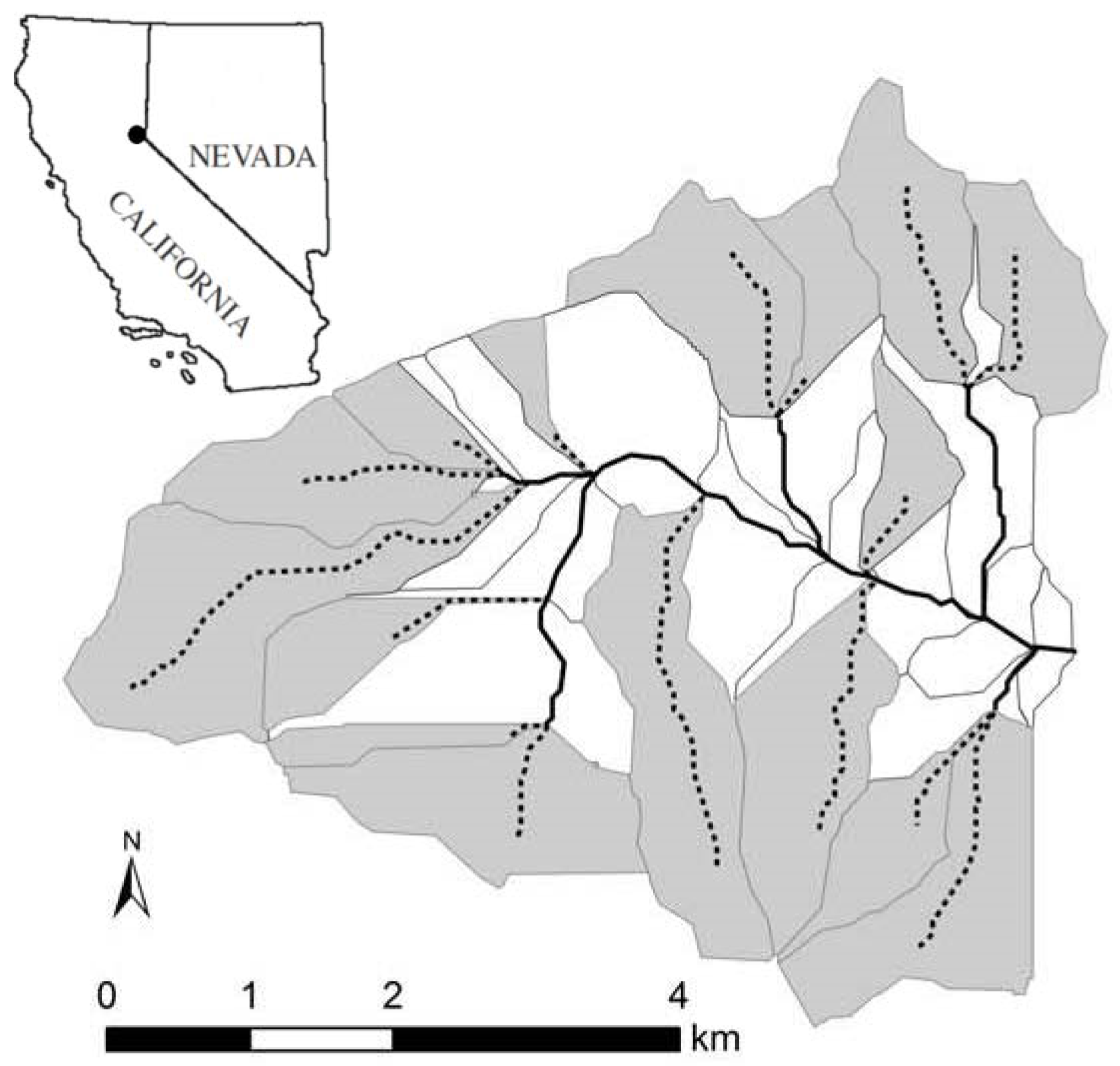
Figure 2.
The calculated breadth (L) based on Equation (8) with different ASNL (B).
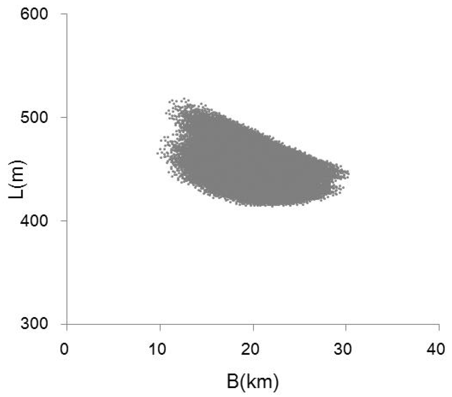
Figure 3.
Plot of log(−dQ/dt) vs. log(Q) derived from the observed streamflow for 51 individual recession events selected over a period of 16 years. The straight line with a slope of 1 illustrates the upper boundary of the plot. This upper boundary is discussed in Section 5.5.
Figure 3.
Plot of log(−dQ/dt) vs. log(Q) derived from the observed streamflow for 51 individual recession events selected over a period of 16 years. The straight line with a slope of 1 illustrates the upper boundary of the plot. This upper boundary is discussed in Section 5.5.

Figure 4.
Separated plots of dQ/dt vs. Q, based on the range of Qmin on a log scale: (a) log(Qmin) < 3.9, (b) 3.9 ≤ log(Qmin) < 4.1, (c) 4.1 ≤ log(Qmin) < 4.3, (d) 4.3 ≤ log(Qmin) < 4.5, and (e) log(Qmin) ≥ 4.5. Gray dots illustrate the recession curves in each range. Two straight dash lines illustrate the upper and lower envelopes. Two black curves are obtained from the solution Equation (2) with the condition of D equal to 4 m (right curve), and 27 m (left curve).

Figure 5.
B vs. D curves calculated using Equation (6). The five black curves are related to five ranges, respectively. The gray zone illustrates the possible range of active stream network. The dash line in the gray zone illustrates the estimated ASNL according to the assumptions stated in Section 4.
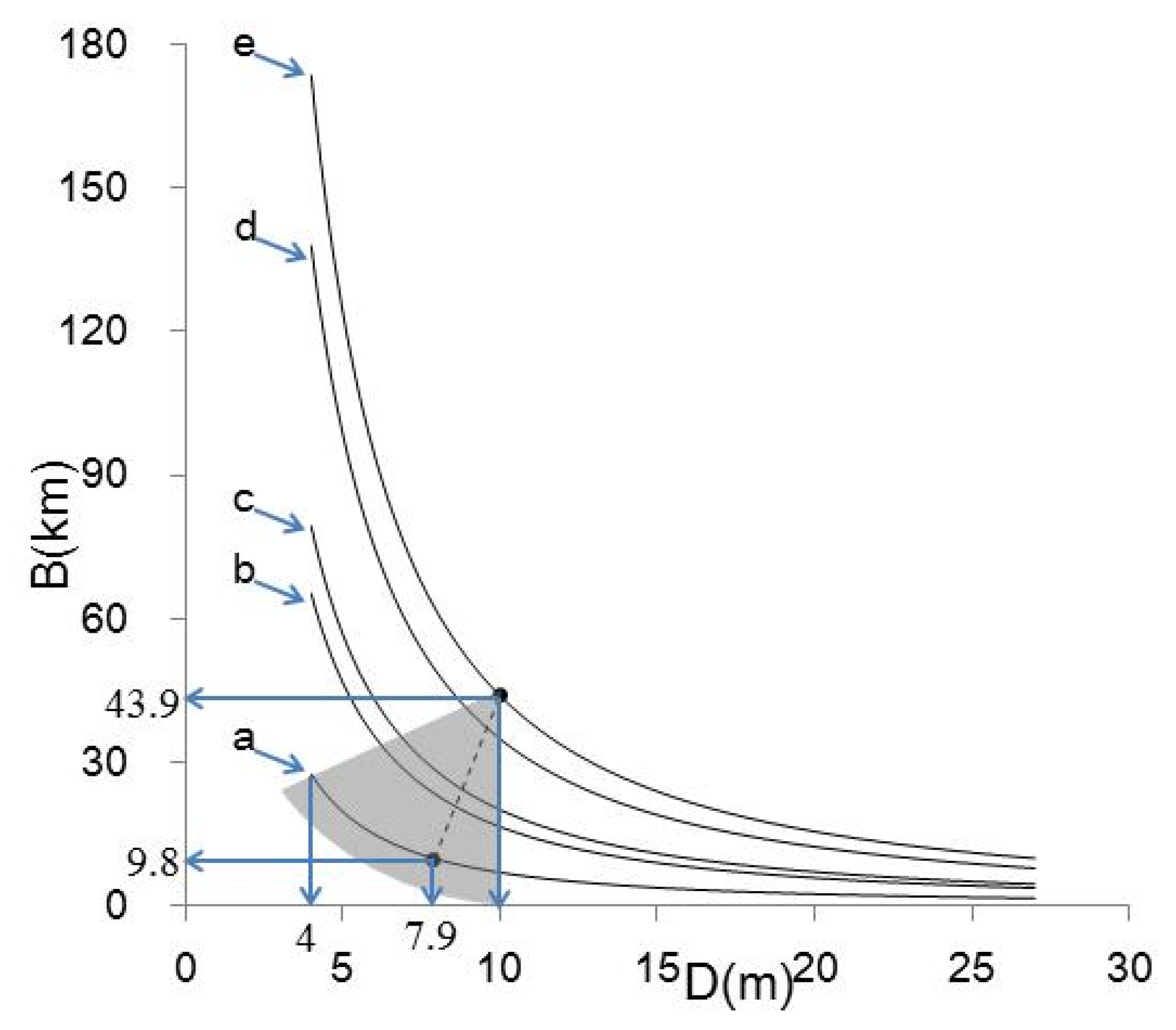
Figure 6.
Sensitivity analysis of estimated ASNL as influenced by variations in k and f: (a) the error bars illustrate the influence of k with a range of 0.026–0.39 m/d; (b) the error bars illustrate the influence of f with a range of 0.08–0.15.
Figure 6.
Sensitivity analysis of estimated ASNL as influenced by variations in k and f: (a) the error bars illustrate the influence of k with a range of 0.026–0.39 m/d; (b) the error bars illustrate the influence of f with a range of 0.08–0.15.

Table 1.
Key values of each plot in Figure 4a–e and estimated ASNL
Table 1.
Key values of each plot in Figure 4a–e and estimated ASNL
| Parameters | a | b | c | d | e |
|---|---|---|---|---|---|
| Range of log(Qmin, m3/d) | <3.9 | 3.9 – 4.1 | 4.1 – 4.3 | 4.3 – 4.5 | ≥4.5 |
| Number of recession curves | 13 | 11 | 13 | 7 | 7 |
| Mean Q (m3/d) | 8054 | 13445 | 18520 | 33041 | 58899 |
| α (d/m6) | 3.16 × 10⁻⁹ | 5.62 × 10⁻¹⁰ | 3.80 × 10⁻¹⁰ | 1.26 × 10⁻¹⁰ | 7.94 × 10⁻¹¹ |
| Range of ASNL (km) | 1.6–27.5 | 3.7–65.2 | 4.5–79.3 | 7.9–137.8 | 9.9–173.5 |
| ASNL (B) estimated from the dash line in Figure 5 (km) | 9.8 | 20.7 | 24.3 | 37.1 | 43.9 |
© 2017 by the authors. Licensee MDPI, Basel, Switzerland. This article is an open access article distributed under the terms and conditions of the Creative Commons Attribution (CC BY) license (http://creativecommons.org/licenses/by/4.0/).
Share and Cite
MDPI and ACS Style
Li, W.; Zhang, K.; Long, Y.; Feng, L. Estimation of Active Stream Network Length in a Hilly Headwater Catchment Using Recession Flow Analysis. Water 2017, 9, 348. https://doi.org/10.3390/w9050348
AMA Style
Li W, Zhang K, Long Y, Feng L. Estimation of Active Stream Network Length in a Hilly Headwater Catchment Using Recession Flow Analysis. Water. 2017; 9(5):348. https://doi.org/10.3390/w9050348
Chicago/Turabian StyleLi, Wei, Ke Zhang, Yuqiao Long, and Li Feng. 2017. "Estimation of Active Stream Network Length in a Hilly Headwater Catchment Using Recession Flow Analysis" Water 9, no. 5: 348. https://doi.org/10.3390/w9050348
Note that from the first issue of 2016, this journal uses article numbers instead of page numbers. See further details here.