Application of Multi-Step Parameter Estimation Method Based on Optimization Algorithm in Sacramento Model


1
Institute of Water Resources and Hydro-Electric Engineering, Xi’an University of Technology, Xi’an 710048, China
2
State Grid Gansu Electric Power Company, Gansu Electric Power Research Institute, Lanzhou 730050, China
*
Author to whom correspondence should be addressed.
Water 2017, 9(7), 495; https://doi.org/10.3390/w9070495
Submission received: 4 May 2017
/
Revised: 24 June 2017
/
Accepted: 3 July 2017
/
Published: 7 July 2017
Abstract
:The Sacramento model is widely utilized in hydrological forecast, of which the accuracy and performance are primarily determined by the model parameters, indicating the key role of parameter estimation. This paper presents a multi-step parameter estimation method, which divides the parameter estimation of Sacramento model into three steps and realizes optimization step by step. We firstly use the immune clonal selection algorithm (ICSA) to solve the non-liner objective function of parameter estimation, and compare the parameter calibration result of ideal artificial data with Shuffled Complex Evolution (SCE-UA), Parallel Genetic Algorithm (PGA), and Serial Master-slaver Swarms Shuffling Evolution Algorithm Based on Particle Swarms Optimization (SMSE-PSO). The comparison result shows that ICSA has the best convergence, efficiency and precision. Then we apply ICSA to the parameter estimation of single-step and multi-step Sacramento model and simulate 32 floods based on application examples of Dongyang and Tantou river basins for validation. It is clearly shown that the results of multi-step method based on ICSA show higher accuracy and 100% qualified rate, indicating its higher precision and reliability, which has great potential to improve Sacramento model and hydrological forecast.
1. Introduction
The Sacramento model is a conceptual hydrologic model, which was proposed by the Sacramento Forecast Center of National Weather Service during the period from the late 1960s to the early 1970s. It has been widely applied to the semi-humid region up to now. What is similar to the Stanford model is that the Sacramento model is a consecutive model, and it includes 17 parameters. As is known to us all, it is essential that the parameter should be correctly determined, or the model will lose its efficiency. Therefore, the parameter calibration of conceptual watershed hydrologic model has always been an important content of the flood forecasting, which belongs to the nonlinear optimization problem.
A lot of work about parameter calibration has been done in recent years. With the development of computer science, various optimization algorithms have been explored to deal with the non-liner functions of the parameter optimization in hydrological models, such as Rosenbrock algorithm [1], Shuffled Complex Evolution-University of Arizona (SCE-UA) [2,3,4,5,6], genetic algorithm (GA) [7,8,9,10], particle swarm optimization (PSO) [11,12], Parallel genetic algorithm (PGA) [10], etc.
However, most of these optimization algorithms are still limited with convergence problems, and need further improvement. The Rosenbrock algorithm and SCE-UA require strict model structure and optimization guidelines, which could be significantly influenced by initial conditions and trapped in local optimum. The GA with strong robustness and versatility can generally solves the analytic expressions of objective functions and constrains, but it often runs into problems of premature convergence or slow convergence. The PSO and improved PSO algorithms also cannot avoid the weakness of slow convergence and may be easily trapped in local extremum.
As the famous conceptual watershed hydrologic model of the United States, there usually exists a large difference between the simulated result and actual measured values in the Sacramento model because of the numerous parameters and their defective calibration. Despite the fact that varied objective functions have been tried to improve the deviation of the simulated results through single-step optimization, the effect is rather limited [13]. Thus, the multi-step parameter calibration method comes into being.
The multi-step automatic parameter calibration method was developed by Terri S. Hogue et al. for the National Weather Service [14]. In the year of 2006, their team analyzed the reliability of the multi-step automatic parameter calibration method, and researched the model’s availability in a variety of climatic and hydrologic conditions [15]. Meanwhile, they cooperated with the Hydrologic Laboratory of National Weather Service and then developed an advanced parameter calibration method. The “in house” National Weather Service algorithm was used to optimize the hydrologic model, and it was applied to the Sacramento Soil Moisture model and SNOW-17 model for streamflow forecasting, which had achieved desirable results. The method can be well adapted to hydrologic model, though it was only used within the forecasting system of National Weather Service before. The achievements of their studies have showed that the multi-step automatic parameter calibration method presents excellent performance in each basin, even though in the complex terrain of the western United States.
As we can see, the traditional optimization algorithm which applied to parameter calibration of the Sacramento model still has a lot of problems such as early maturing and slowly convergent speed. Besides, the traditional methods may be easy to fall into the local optimum, and its simulative fitness is poor. In view of the above limits, this paper firstly applies the immune clonal selection algorithm (ICSA) based on artificial immune system in the parameter estimation of Sacramento model, which is more accurate and has fast convergence. We pick the artificial hydrological data from the particular water basins to verify the accuracy and performance of ICSA, and compare the results with other three algorithms, i.e., SCE-UA, PGA, and Serial Master-slaver Swarms Shuffling Evolution Algorithm Based on Particle Swarms Optimization (SMSE-PSO). Then, based on the ICSA, we improved the multi-step parameter calibration method in order to increase the accuracy of the Sacramento model simulation, and give out the detailed evaluation of the simulation results which are obtained from the particular water basins.
2. Materials and Methods
2.1. Immune Clonal Selection Algorithm
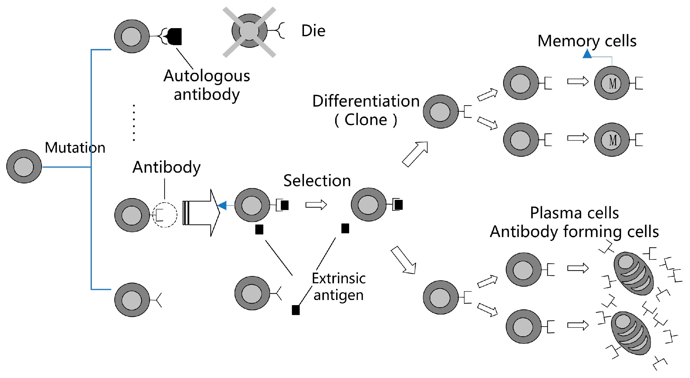
Burnet and Talmage [16,17] proposed the famous antibody clonal selection theory in 1957, of which the basic principle is described as: the antibody is a natural product and exists on the cell surface in the form of receptor; the antigen selectively reacts with antibody. The reaction of antigens and corresponding antibody receptors leads to the clonal expansion of cells, of which some differentiate into antibody forming cells and others differentiate into immune memory cells to participate the following secondary immune response. In this process, the cells activate, differentiate and proliferate through clone to increase the number of antibodies, and finally clear the antigens by immune response. Therefore, the clonal selection is dynamic process of self-adaption to antigen stimulation in biology immune system, through which the generated biological features of study, learn and antibody diversity can be prominent references to the artificial immune system. At present, the most classic simulation method to describe the mechanism of antibody clonal selection is the immune clonal selection algorithm (ICSA) raised by De Castro in 2000 [18], and the follow-up researchers also have developed several advanced clonal selection algorithms from diverse angles [19]. The ICSA simulates the maturity process of antibody population through clone, hypermutation and selection. The principle diagram of ICSA is shown in Figure 1.
The ICSA has splendid performance in searching and finding solutions irrelevant to problem. The essence of clone in ICSA is to produce a mutant solution group near the candidate solutions of every generation according to affinity, which enlarges the search range of solutions (i.e., it enlarges the diversity of antibodies). The simultaneous global search and local search effectively avoid being trapped in local minimum and premature convergence of evolutionary programming, while the clone selection accelerates convergence. The process of clonal selection can be recognized as: the problem in low-dimensional space is transferred into higher-dimensional space for solution, then the solutions are projected back to low-dimensional space. The detail of ICSA method can be seen in the reference [20].
The solution procedure of ICSA is showed as below.
Step 1: Population initialization: suppose the population size of antibody is N, the clonal size of antibody is , the mutation probability is , and the recombination probability is . Then randomly generate the initial population , in which the matrix contains the all parameters of the Sacramento model, and set the mature condition of affinity (that is the objective function), the currently iterations is .
Step 2: Calculate the affinity of antibody population , if the mature condition of affinity is satisfied, then output the antibody with highest affinity and stop the algorithm. Otherwise, go to the step 3.
Step 3: The cloning operation of antibody population : , then obtain the antibody population .
Step 4: The immune gene operation of antibody population : , then obtain the antibody population .
Step 5: The selection and recombination of antibody population : , then obtain the antibody population .
Step 6: Calculate the affinity of .
Step 7: According to the size of affinity, perform the clonal selection operation towards the antibody population and : , then obtain the next generation antibody population .
Step 8: , then go back to the Step 2.
2.2. The Parameter Estimation in Sacramento Model for Artificial Generated Data
2.2.1. Sacramento Model
The Sacramento model is a conceptual model described by a series of mathematical expressions with certain physical concepts, which is a comprehensive river rainfall-runoff model used to simulate the hydrological cycle based on the soil moisture, infiltration, drainage and evapotranspiration characteristics. Each of its variables represents an independent and understandable characteristic of the hydrological cycle, and the model parameter can be derived from the rainfall, flow data and the basin characteristic. The Sacramento model consists of three parts: evapotranspiration calculation, runoff-yield calculation and flow-concentration calculation [21]. The model structure [22,23,24] is showed in Figure 2.
As we can see, the soil is divided into upper and lower zones, and the water storage of each layer can be divided into the tension water and free water [25]. The rainfall first supplements the evenly distributed tension water in the upper zone, and then supplements the free water in the upper zone. The tension water subsided for evapotranspiration, and the free water will infiltrate into the lower zone and generate the lateral interflow. Besides, the Evapotranspiration calculation mainly accounts for five kinds of evapotranspiration, including the amount of evaporation on an impervious area , tension water evapotranspiration in the upper zone , free water evapotranspiration in upper zone , evapotranspiration on the water area of the watershed , tension water evapotranspiration in the lower zone .
It is a continuum model including 17 parameters, in which PCTIM, ADIMP and SARVA are three parameters of the direct runoff, UZTWM, UZFWM and UZK are three parameters of the water capacity of upper zone, ZPERC and REXP are the parameters of percolation, PFREE, LZTWM, LZFSM, LZSK, LZFPM, LZPK, RSERV, SIDE and SSOUT are the 9 parameters of water capacity of lower zone, and it is mainly adapted to semi-arid and semi-humid regions. Table 1 lists the value range and physical meaning of parameters in Sacramento model.
2.2.2. Objective Function
Objective functions are used to evaluate the consistency of simulated flow with measured flow, and different objective functions correspond to different characteristics in hydrologic process. In this paper we choose the following objective function based on comprehensive considerations of overall water quantity balance and the consistency with flow process:
In Equation (1), is the parameter to control the flow magnitude (threshold value); is the measured flow and is the average measured flow; is the calculated flow from the model and is the average calculated flow; is the number of flood occurrences of which , and is the number of flood occurrences of which ; is the length of calibration data; is the weight coefficient for different objective functions. The Equation (1) shows that different and can be used for different application requirements.
2.2.3. Study Basin
We choose the Dongyang river basin above Balihutong hydrological station and the Tantou river basin above Yihetantou hydrological station between the Yellow River Huayuankou and Sanmenxia interval, as the study water basin, which are shown in Figure 3.
The Dongyang basin is a semi-humid and semi-arid region with the area of 537 km2 and average annual rainfall of 550 mm, including several important rainfall stations such as Shibandao, Hengheng and Huangyuan. In this paper we take the average rainfall of the three stations as the rainfall of the entire Dongyang basin, and take the flow of Balihutong station as the basin outflow. Also, the Tantou basin is a semi-humid and semi-arid region with the area of 1695 km2 and average annual rainfall of 580 mm, including several important rainfall stations such as Taowan, Miaozi, Baitu, and Tantou. Similarly, the average rainfall of the four stations is taken as the rainfall of the entire Tantou basin, and the flow of Tantou station is taken as the basin outflow.
2.2.4. The Generation of Artificial Data (the Ideal Data)
In order to judge whether the ICSA method is practical and available for the Sacramento model parameter calibration, we use the artificial data to calibrate the parameter for validation. The detailed procedure is showed as below.
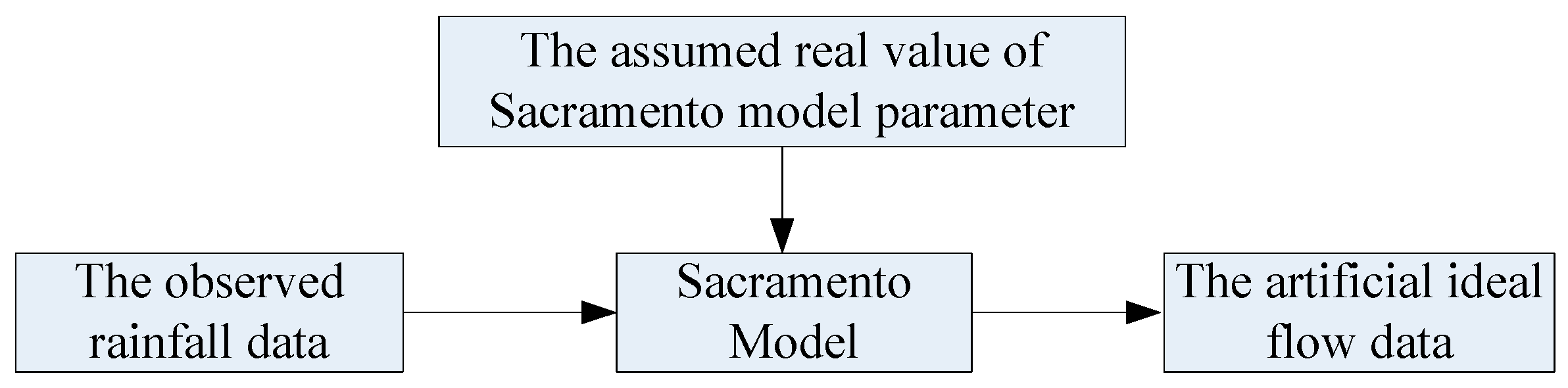
Step 1: Suppose a set of parameter value as the real value of the model parameter, and take the observed rainfall data as the input of model, then we can obtain a set of ideal flow data, that is to say, the artificial ideal flow data.
Step 2: Take the observed rainfall data as the input, and take the corresponding ideal flow data as output of model to calibrate the parameter, then we can obtain a set of calculated parameter values and corresponding calculated flow data.
Step 3: The real parameter is compared with the calculated parameter, and the ideal flow data is compared with the calculated flow data, then conduct analysis and evaluation.
The framework diagram of artificial ideal data generation is showed in Figure 4.
2.2.5. Parameter Estimation
In order to compare the performances of different algorithms in parameter estimation of Sacramento model, we assume a series of artificial generated data to be the real values of the parameters for the validation of parameter estimation. The study basins are aforementioned Dongyang and Tantou river basins. Then we utilize the rainfall and evaporation data of two floods (No.820801 and No.820730) and Sacramento model to simulate these two floods, and employ SCE-UA, PGA, SMSE-PSO, ICSA to calibrate parameters. Our PC infrastructure is that the CPU is Intel Core i7-3537U CPU, the CPU Clock Speed is 2.50 GHz, the Operating System is Windows 8.1, and the Programming Language we used is Java. We set the initial population size = 80, the largest iterations = 300, the precision of coding = 0.001, = 800 m3/s, = 0.6, so as to ensure the comparison of the four algorithms is under the same condition. We run each algorithm for 5 times and obtain the optimal results according to objective functions. Detailed results are shown in Table 2 and Table 3.
Here we use the Nash-Sutcliffe model efficiency coefficient (NSE) [26] as the evaluation criterion, and it is calculated as:
in which denotes the number of flood time periods, denotes the simulated flow, denotes the measured flow, denotes the measured average flow.
Table 2 gives out the parameter estimation results of the artificial generated data. We can see that the calibration values are very close to the assumed real values with small errors, indicating that the optimal results of all four algorithms can converge to real values.
Table 3 clearly demonstrates the parameter calibration performances of the four algorithms. All four algorithms have converged to real values with NSE approaching very close to 1. The running time and iterations directly reflects the efficiency and convergence rate of the employed algorithm. For each algorithm, the running time and iterations of No.820801 Flood is smaller than that of No.820703 Flood, which is resulted from shorter last time and thus simpler calculation of the No.820801 Flood. As for the same flood, the running time and iterations of SCE-UA are the largest among four algorithms, while that of the proposed ICSA are the smallest. Clearly, the rank of efficiency and convergence rate of the four algorithms is ICSA > SMSE-PSO > PGA > SCE-UA. Besides, the ICSA owns the smallest objective function values in both two floods (2.1943 and 8.4972, respectively), implying the best consistency of the simulated results and real values.
From Table 2 and Table 3 we can conclude that ICSA shows the best parameter estimation performance among all four algorithms in the experimental Sacramento model, with the highest efficiency, precision, and convergence rate. Besides, we can find that there exists some difference between the parameter calibration results obtained from each algorithm. Although the difference is quite small and the artificial ideal data were used to calibrate the parameter, it still leads to a large difference in the objective function value, and the NSE does not reach the optimal value yet. This may be caused by these two reasons, on the one hand, it may be a problem of optimal algorithm, for example, the algorithm is not good enough, or the setting termination condition is not reasonable (the maximum iterations is too small). On the other hand, the uncertainty of the model structure may be the primary cause, particularly the parameter uncertainty, in other words, although the ideal data is used for parameter calibration, if the model structure has any fault, it will still result in errors. Therefore, we will give a detailed analysis of parameter uncertainty in the next section.
2.2.6. The Analysis of Parameter Uncertainty
The parameter uncertainty analysis consists of two contents, the sensitivity analysis and the equifinality, and this paper will also analyze the parameter uncertainty through the two aspects.
The Parameter Sensitivity Analysis
The sensitivity analysis is to study the model response caused by the model parameter variation, and focus on the consideration about the contribution of model parameter variation to the model output, in order to identify whether the parameters have a great impact on the model response or not. The sensitivity analysis method applied to hydrologic model can be generally divided into the local sensitivity analysis method and global sensitivity analysis method.
Local sensitivity analysis (LSA) method pays attention to the impact on the model output caused by single parameter, with the advantage of simple, fast and strong operability, among which the perturbation analysis method [27] is widely used because of its simple and practical character. However, the variation of one parameter value may impact the sensitivity of the other parameters, due to the poor consideration about the interaction of all parameters, the LSA method is lack of stability and there are also some limitations.
While in the global sensitivity analysis (GSA) method, the impact on the model output caused by the change of multiple parameters and the interaction of all parameters can be simultaneously taken into account, and we can obtain a comprehensive understanding about the sensitivity of each parameter, which is applicable for the hydrologic model with multiple parameters. For example, the GLUE method [28], the Sobol method [22,29], the RSA method [30] and the RSMSobol method [31], all of them are the commonly used GSA method.
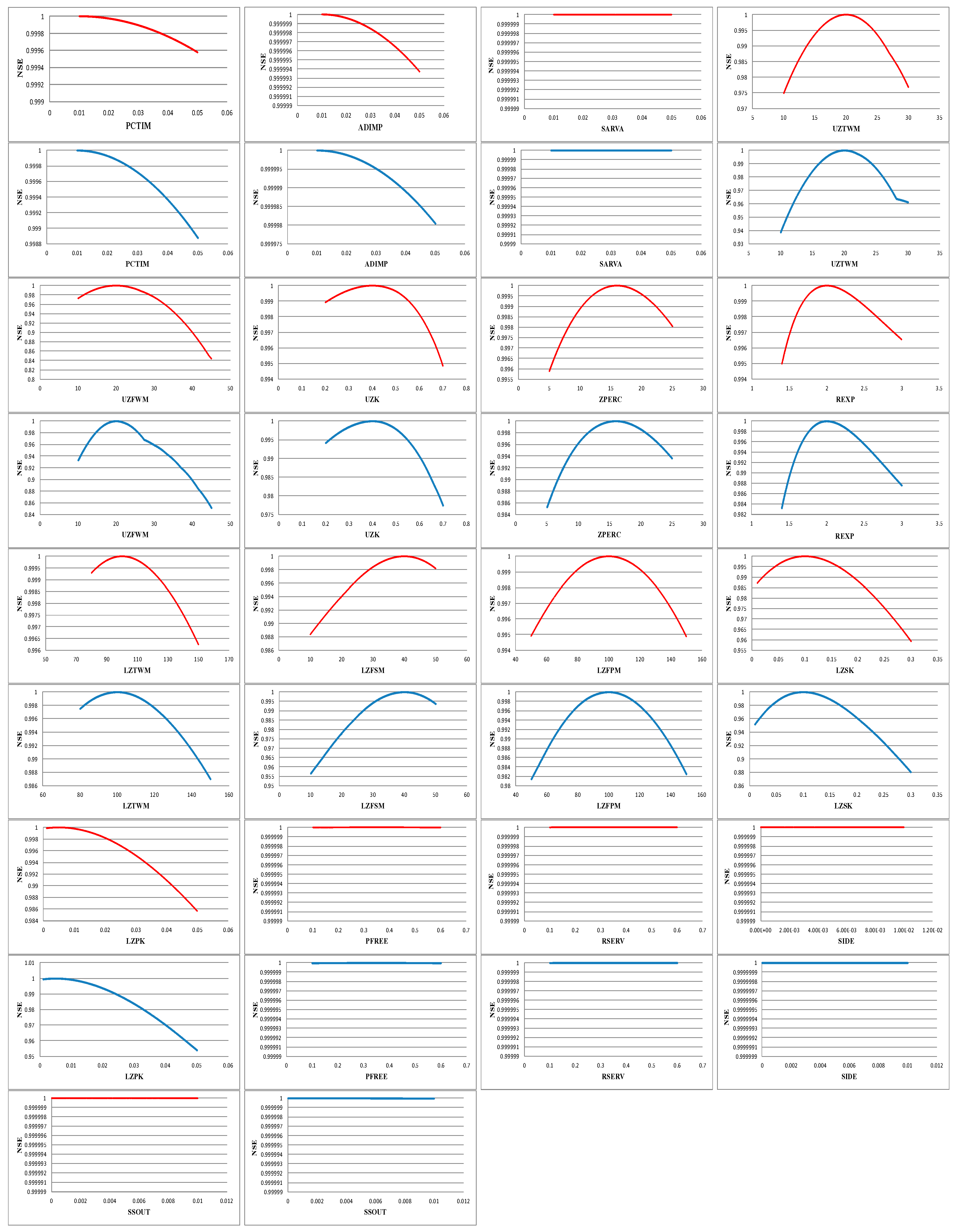
In this paper, take the two floods showed in Table 2 as examples, we first apply the perturbation analysis method to the 17 parameters of Sacramento model for single-parameter sensitivity analysis, that is to say, suppose that all of parameters are at their true value, just change one parameter value according to its value range at a time, fixing the remaining 16 parameters invariable, then the corresponding NSE can be obtained and the NSE curve as shown in Figure 5.
In the above figures, red curve represents the simulated results obtained from the No.820801 flood in Doyang river basin, and the blue curve represents that of the No.820730 flood in Tandou river basin. As to these two floods, the range of corresponding NSE changes little with the variation of the parameter. For the No.820801 flood (the red curve), we can find that the parameter whose corresponding NSE with largest variation range is UZFWM, it is varying from 0.84 to 1, and the corresponding NSE of the other 16 parameters are all no less than 0.955. Thus, the parameter UZFWM is the most sensitive parameter to this flood, while the parameter PCTIM, ADIMP, SARVA, UZK, ZPERC, REXP, LZTWM, LZFPM, PFREE, RSERV, SIDE and SSOUT are almost insensitive, all of them has the NSE which is no less than 0.994. For the No.820730 flood (the blue curve), the parameter UZFWM (with NSE between 0.85 to 1) and LZSK (with NSE between 0.88 to 1) are the parameters whose NSE has largest variation range, so these two parameters are more sensitive than others to this flood. The corresponding NSE of the remaining parameters are all larger than 0.935, particularly the parameter PCTIM, ADIMP, SARVA, PFREE, RSERV, SIDE and SSOUT has the NSE no less than 0.9988, so these parameters are almost insensitive to this flood.
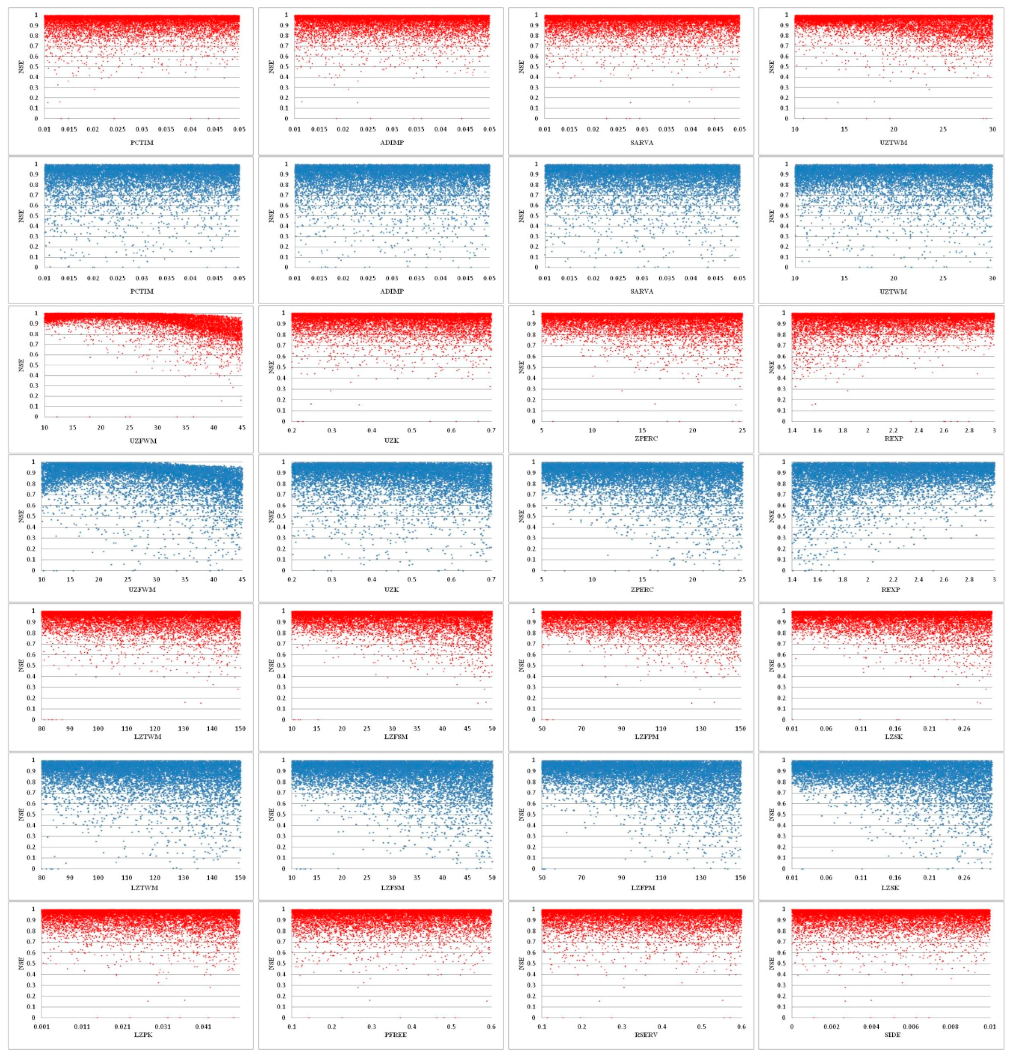
Besides, the Monte Carlo Sampling based GLUE method is also used for parameter sensitivity analysis from a global perspective, which means all of the 17 parameters will be changed according to their own value range, 10,000 groups of parameters will be selected randomly to conduct simulation, and the parameter value and its corresponding NSE are showed in Figure 6.
The same to Figure 5, the red point represents the simulated results of No.820801 flood in Dongyang river basin, and the blue point represents the No.820730 flood in Tantou river basin. Since the GLUE method assumes that the parameters are uniformly distributed within their acceptable range, most of the parameter values in the figures are uniformly distributed in their values range. As to the No.820730 flood (red figure), we can see that most of points fall in the area in which , the most sensitive of all is the parameter UZFWM, the corresponding NSE of which obviously decrease when the parameter value is greater than 30. In addition, with the increase of the parameter value of UZTWM, ZPERC, LZFSM, LZFPM, LZSK and UZFWM, the probability of their NSE falling into the area of will decrease, while the parameter REXP has the opposite tendency. For the No.820730 flood (blue figure), most of parameters value have corresponding NSE between 0.8 and 1, and the parameter UZFWM is still the most sensitive one to this flood, the corresponding NSE will decrease when it’s greater than 25. Meanwhile, the increase of the parameter ZPERC, LZFSM, LZFPM and LZSK will result in a decrease of NSE, while the parameter REXP still holds an opposite tendency.
Note that all the simulated results were just applicable for the particular two floods. Based on the analysis results of the above two methods, while the ideal data are used for parameter calibration, we can find that the sensitivity of the same parameter is not the same when applied to the different basins or different floods. That is to say, the sensitivity of the same parameter is affected not only by flood conditions, but also by the different basins applied. In addition, the results obtained from the LSA method and the GSA method are also not the same, while multiple parameters are simultaneously taken into consideration, the single-parameter sensitivity may be changed because of the interaction or the complementarity between the parameters.
The Model Equifinality Analysis
The equifinality [32] of the model means that for the same model structure and model input, there will be multiple groups of optimal parameters which make the model output have the same accuracy. The reasons causing equifinality may be the data uncertainty, the model structure uncertainty, the complementarity between the model parameters, the randomness of the parameters, and the multi-extremum of objective function, etc.
As for the ideal data, Duan et al. [2] assumed the model is correct, the model input and output will be non-error, and there will not exist equifinality problem under this situation. While some other hydrologists like Beven et al. [33] hold the different opinion, they believe that even under the ideal condition and both the input and output data are correct, it may still results in the equifinality problem if there exists any error in the assumed model structure.
Like the opinion of Beven et al. we believe that when the ideal data are used for parameter calibration of different floods, if the assumed model structure is non-correct, it will cause the error in results. However, we can not prove that whether the model structure is correct or not. Here we assume that for a flood with the ideal data for parameter estimation, if there is no error in the input and output data and the model we chose is applicable and proven by many scholars, the equifinality effect caused by model structure will be less than the error caused by the optimization algorithm (optimization ability and optimization condition setting).
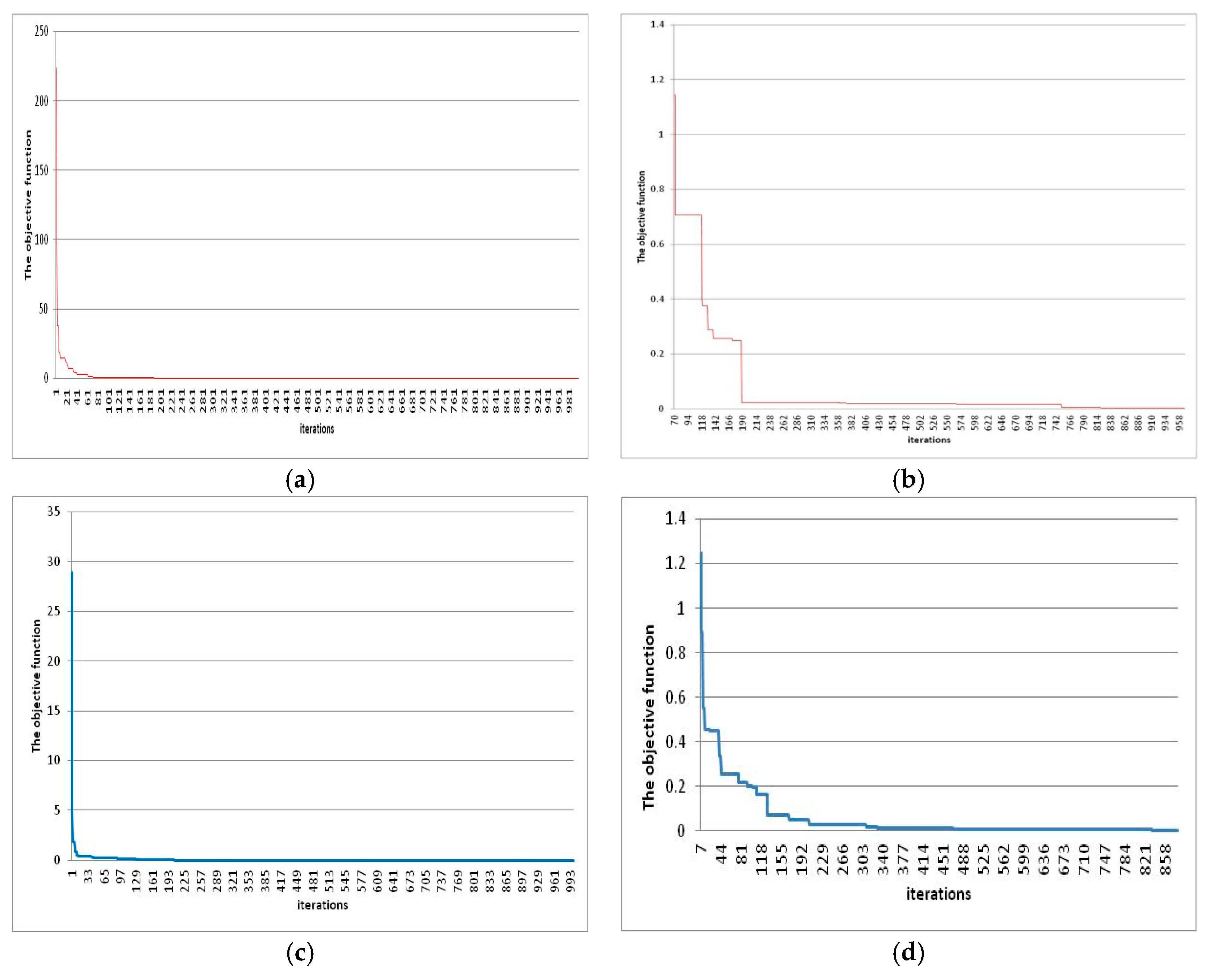
As shown in Table 2 and Table 3, in order to compare the pros and cons of the four algorithms, the initial population size and the maximum iterations we set in our algorithms were only n = 80 and k = 300. In order to validate the above assumptions, here we change them to n = 500 and k = 1000, and observe the results of simulation.
As shown above in Figure 7, when the setting condition of the optimization algorithm were changed, the value of objective function obtained by the ICSA will eventually stabilized at around 0.0035 and 0.0043, respectively.
Therefore, we can draw a conclusion that the main reason resulting in the difference of the parameters and the objective function values is the optimization condition setting of the optimal algorithm, which makes the objective function do not converge to the optimal value, while the equifinality is not the main reason.
2.3. Multi-Step Parameter Estimation Method
The Equation (1) gives out the traditional single-step parameter estimation method. Since each parameter of the 17 parameters in Sacramento model has its own physical meaning and combines to other ones, different types of the parameters should use corresponding estimation principles. As a result, the simulated results of single-step method often have large deviation with the actual measured results. Although using different objective functions could raise simulation accuracy, the improvement is rather limited [34]. Therefore, in this paper we present the multi-step parameter estimation method as solution. The parameter estimation of Sacramento model needs three steps as follows.
Step 1: The following objective function is utilized for all parameters:
in which denotes the simulated flow, and denotes the measured flow. Step 1 emphasizes the underground runoff related parameters in the flood process, including , , , , , . Meanwhile, estimation for all parameters benefits the relativity weakening of the surface and underground water runoff related parameters.
Step 2: Set the underground runoff related parameters obtained in Step 1 as constants, and use the following objective functions for parameter estimation:
in which and are the simulated and measured flows, is the number of simulation days or number of flood time periods. Step 2 emphasizes the surface water runoff related parameters in the flood process, including , , , , , .
Step 3: Set the surface water runoff related parameters obtained in Step 2 as constants, and use the Equation (3) as objective function.
3. Results
Combining the ICSA and multi-step method discussed in Chapter 2, we present the ICSA based multi-step parameter estimation method in Sacramento model. We pick the data of 10 floods of Dongyang basin (1963–1990) and 32 floods of Tantou basin (1970–1990) for application examples. Among all the flood data the 7 floods of Dongyang basin and 25 floods of Tantou basin are simulated for parameter estimation, while the others are used for validation. Also, the single-step parameter estimation method with the objective function of Equation (3) is also given for comparison. Detailed results are demonstrated in Table 4.
The flood forecasting accuracy is determined by the results of parameter estimation and also reflects the effect of the parameter estimation method. Here we use three evaluation criterions, i.e., time root-mean-square of flow (TRMS), NSE, and bias (%BIAS). Lower TMRS reflects better dispersion degree, and is calculated as:
The %BIAS is calculated as:
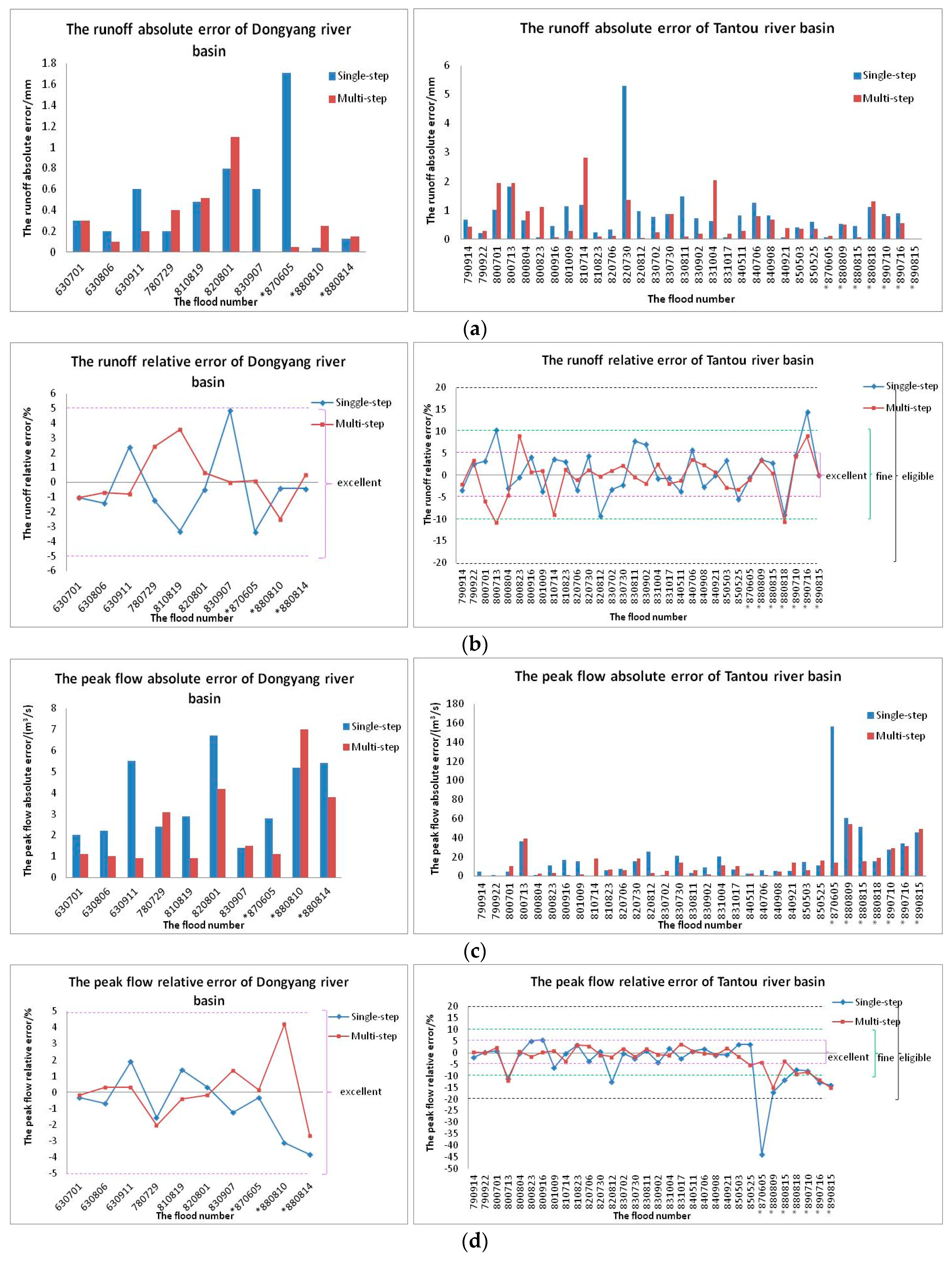
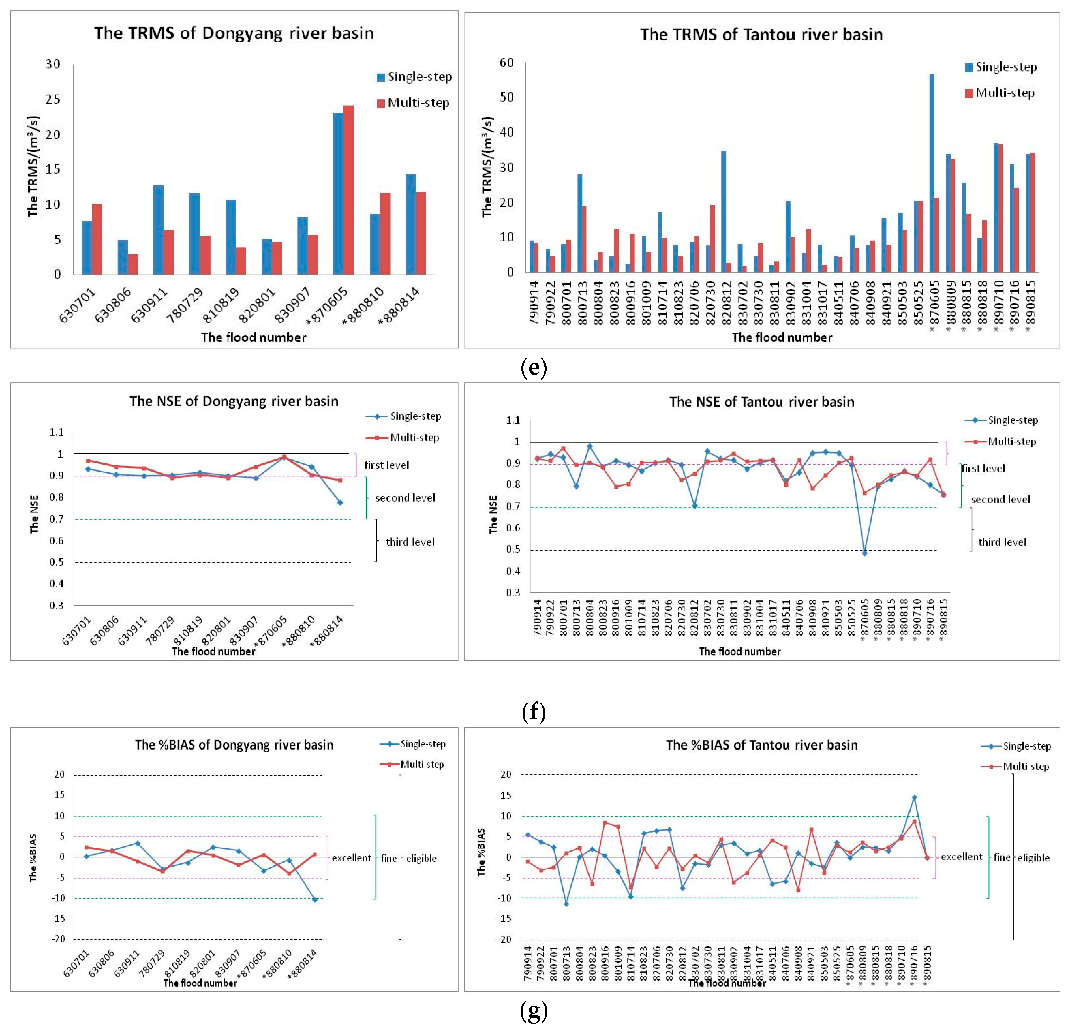
Then we use the remaining floods data to validate and evaluate flood forecasting accuracy and thus the parameter estimation results by above three criterions. The flood simulation results (runoff & peak flow) and the accuracy statistics of both single-step simulation and multi-step simulation are illustrated in Figure 8. Note that the “*” represents flood for validation.
From the above Figure 8a–d, we can find that, for the Dongyang river basin, the absolute and relative errors of runoff, and the absolute and relative errors of peak flow obtained from the single-step method are below 1.71 mm, ±4.88%, 6.7 mm and ±3.84%, and those criteria obtained from the multi-step method are 1.1 mm, ±3.59%, 7 mm and ±4.22%. Besides, for the Tantou river basin, those criteria obtained from the single-step method are below 5.3 mm, ±14.38%, 156.39 mm and ±43.81%, and those criteria obtained from the multi-step method are below 2.83 mm, ±10.88%, 54.13 mm and ±15.08%. Therefore, we can see that the results of flood *870605 in Tantou river basin obtained from single-step method is not qualified.
Then from the Figure 8e, for the 10 floods in Dongyang river basin, the TRMS of 7 floods obtained from the multi-step method is better than the single-step. Besides, for the 32 floods in Tantou river basin, the TRMS of 20 floods obtained from the multi-step method is better.
As we can see from Figure 8f–g, for Dongyang river basin, the %BIAS from single-step method has the maximum larger than ±10% and the average value of 7.47%, the %BIAS below ±3% account for 70%; the %BIAS from multi-step method has the average value of 3.07, and the values below ±3% account for 80%. For Tantou river basin, the %BIAS from single-step method has the maximum nearly ±15% and the average value of 2.75, the %BIAS below ±5% account for 68.75%; the %BIAS from multi-step method has the average value of 2.05, and the values below ±5% account for 71.88%.
We compare the error results of single-step and multi-step flood simulations with the permissible error of “Forecasting norm for hydrology intelligence of China” (SL250-2000). For the Dongyang river basin, the evaluation criterions of single-step and multi-step simulations are all within the accepted error range (±20%), thus the model parameters can be recognized as basically reasonable. Note that, all evaluation criterions of multi-step simulations are better than that of single-step simulations. Through the comparison of NSE, it is found that among the ten simulated floods for validation, seven floods reach the first level and three reach the second level (according to SL250-2000) for both single-step and multi-step methods. That is to say, both single-step and multi-step method for Dongyang river basin reach qualified level.
However, for the Tantou river basin, the relative error of flood flow peak of No.870605 flood in single-step simulation exceeds the permissible error, indicating that the flood forecasting of No.870605 by single-step method is unqualified. Also, the other evaluation criterions of single-step method are all worse than that of multi-step method. Through the comparison of NSE, we can see that among the 32 simulated floods, for single-step method, 15 floods reach the first level, 16 reach the second level, and 1 is unqualified; for multi-step method, 17 floods reach the first level, 15 reach the second level, and none is unqualified.
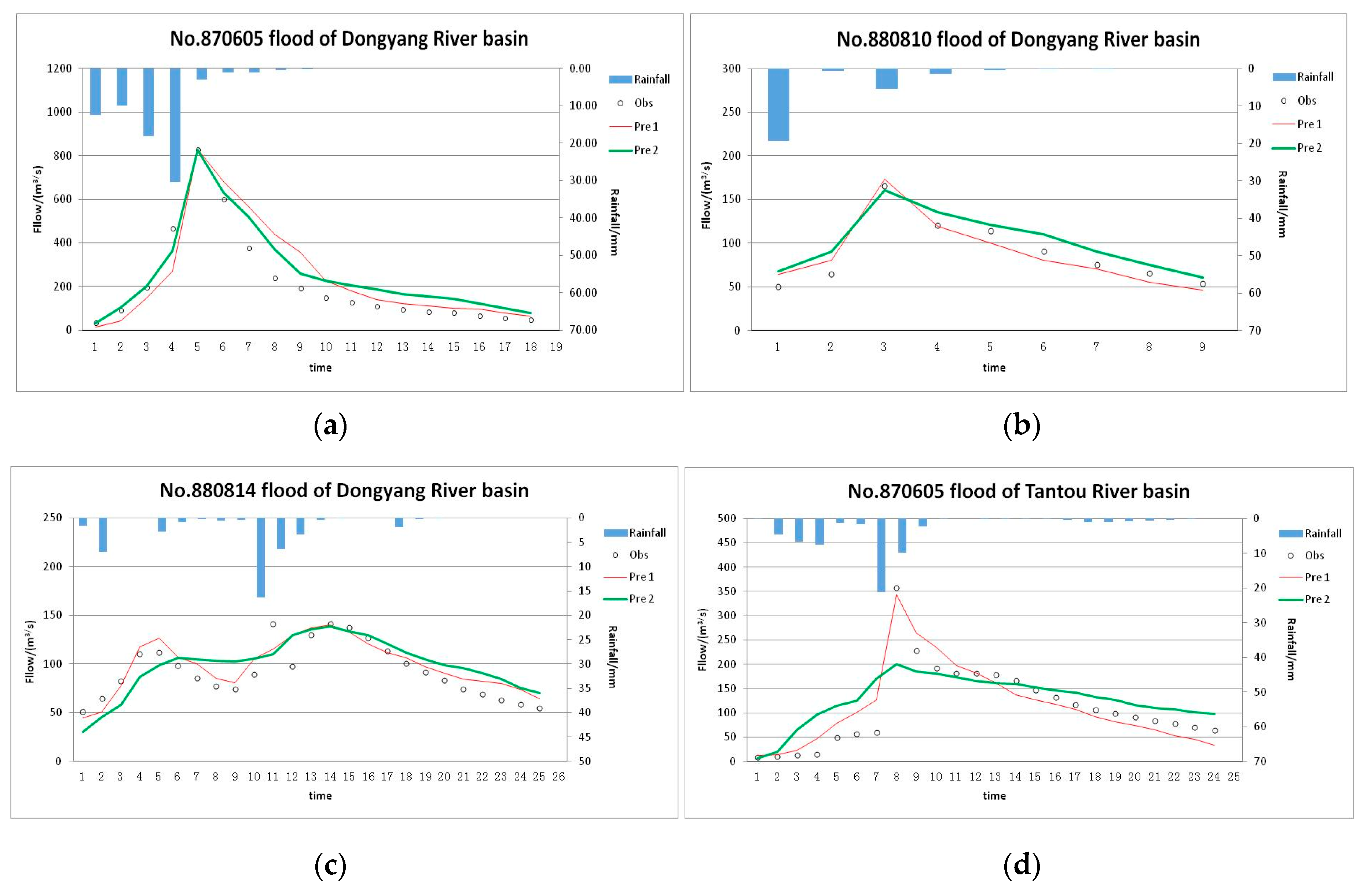
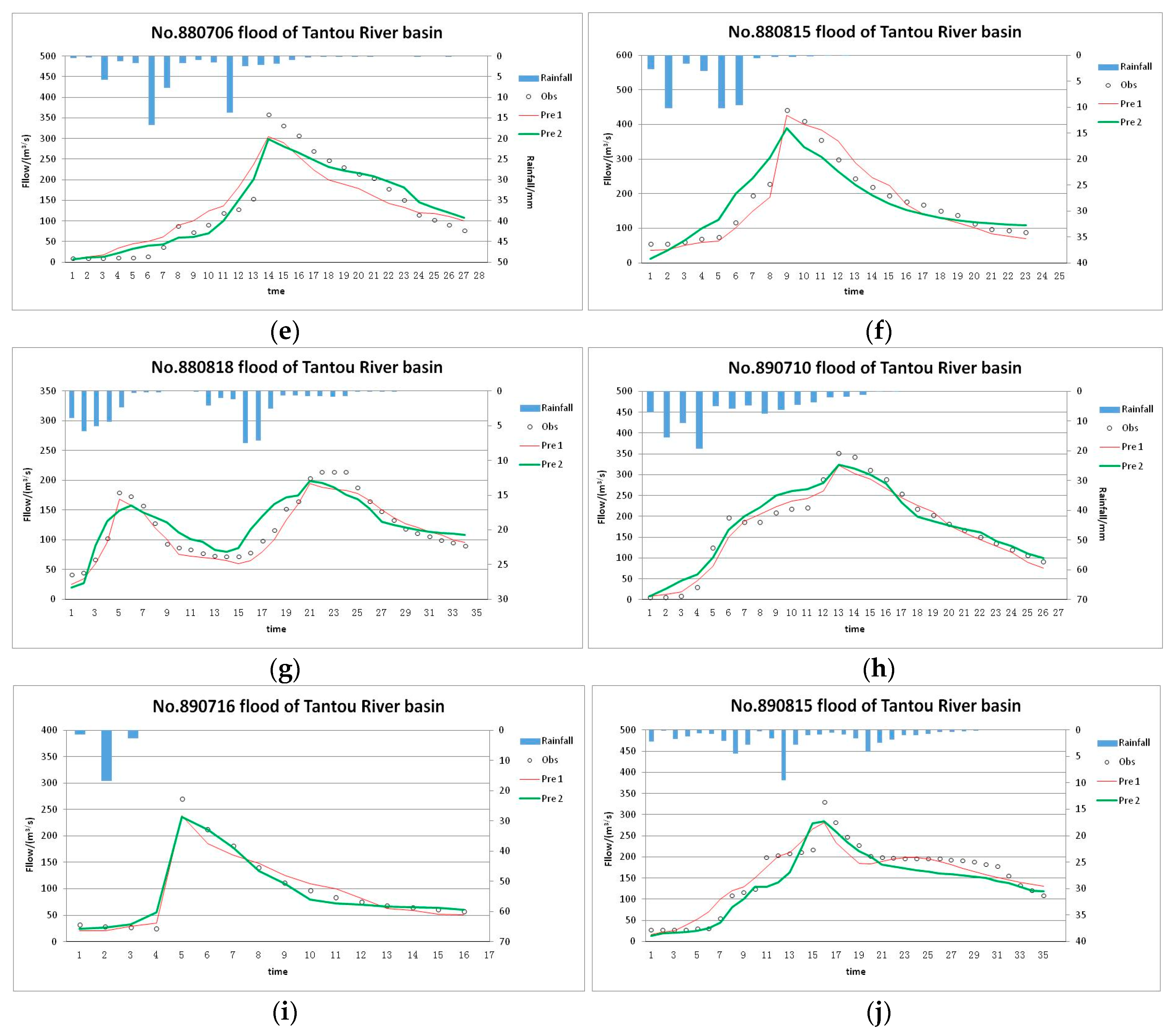
The simulation results comparison of flood forecasting between single-step method and multi-step method is showed in Figure 9. Pre1 means the simulation results which obtained from the multi-step method, while Pre2 means the simulation results which obtained from the single-step method.
4. Discussion
In this paper, both the artificial generated data and the actual flood data are used to calibrate the parameter of Sacramento model, although we have improved the flood prediction accuracy by analyzing the parameter calibration process under these two conditions, there are still some difficult issues required further discussion.
(1) We first use the ICSA and the other three optimization algorithms for Sacramento model parameter calibration based on the artificial generated data, the initial aim of which is to validate the practicability and better performance of ICSA by comparing the simulated results of the four algorithms. During this process, although the artificial generated ideal data are used for parameter calibration, there still exists some bias in the parameter value, objective functions and the corresponding NSE, which results in the search for the origin of the bias. Therefore, the analysis of the bias sources under the ideal condition should be an aspect that needs to be further studied. Many scholars have validated their own opinions from the view of their specific example, but there is no confirmation of others’ results by using their own view. This indicates that different models, basins and input conditions may have certain impacts on the bias, in one case, the bias caused by the model structure is larger than that caused by the optimization algorithm, whereas in another case it can be the opposite. Thus, the causes of the bias should be analyzed according to the specific application conditions.
(2) While in the actual flood simulation and prediction, the ICSA is combined with the multi-step parameter calibration method, and multiple criteria are used for evaluation, which have improved the prediction accuracy of Sacramento model. However, we haven’t made the analysis of the prediction uncertainty, the main reason is that we have made fewer studies in this field, and there are only some immature views. First of all, the current parameter uncertainty analysis are mainly focused on the simulation process based on daily streamflow data [22,23,24,35] and then give the calibrated parameter set, while the probability forecasting method are used for the flood event simulation process [36], in which the parameter uncertainty analysis are avoided. The flood event model parameter calibration is to select a group of parameters from multiple floods by using a kind of evaluation criterion, although the group of parameters is receivable to the multiple floods, it may not be credible for one of the floods. From the view of equifinality, this kind of parameter should also be parameter set, as for the multiple different floods, the parameter variation range will be larger than that of the single flood, thus, it’s difficult to simultaneously analyze the parameter uncertainty of multiple floods. Because of the model equifinality, the model parameter become the parameter set, in order to reduce the selection range of the parameter and improve the parameter selection efficiency, Guo et al. [37,38,39] proposed to adopt the multi-objective algorithms for parameter calibration and uncertainty analysis. This method provides an idea for us to solve the model equifinality problem of multiple floods, we can utilize multiple objective functions and criteria to evaluate the simulation results of each flood, and simultaneously adopt multiple criteria to conduct comprehensive evaluation of the simulated results of all floods. Then the double-evaluation will be formed to reduce the space of parameter set so that we can improve the parameter selection accuracy.
5. Conclusions
According to the analysis and studies about the commonly used algorithms and methods for parameter calibration of Sacramento model, we can find that there are still some problems in the practical application of the optimization algorithms, for example, the premature convergence, easy to fall into local optimum, or slow convergence. The traditional single-step parameter calibration method also has disadvantages of lower simulation and prediction accuracy, and poor performance. In view of all these problems, this paper presented a Multi-step parameter calibration method based on the ICSA for Sacramento model in order to improve the accuracy and stability of parameter calibration.
First of all, we give a brief introduction about the ICSA and Sacramento model basic theory, and the 17 parameters of the Sacramento model as well as their value range are also showed in the paper. Besides, according to the different flow magnitude, different objective functions of optimization algorithm for Sacramento model parameter calibration are set up. Meantime, combined with the specific characteristics of the Sacramento model, the ICSA is used to solve the parameter calibration problem for Sacramento model, and the detailed solution steps are proposed.
Then, take the Dongyang river basin and Tantou river basin as typical study basin, and a flood is selected from each of basins for parameter calibration based on the artificial generated data. The detailed procedure of artificial data generation is also introduced in this paper, we adopt the corresponding rainfall, evapotranspiration and the initial soil moisture data of the flood as the input of Sacramento model, and assumed a group of parameter value as the real value of parameter to generate a group of flow data. After that, we still use the previous input data, and take the artificial generated flow data as the output to calibrate the parameters. Under the same condition, the ICSA, SMSE-PSO, PGA and SCE-UA are all used to solve the parameter calibration problem of the selected two floods based on the artificial generated data, and the objective functions and the NSE are taken as the evaluation criteria. The results showed that to these two floods, whether from the view of convergence speed, the objective functions or the NSE, the ICSA is the most excellent algorithm. Thus, we can validate that the ICSA is applicable and practical for Sacramento model parameter calibration and provide a better solution algorithm for the multi-step parameter calibration method.
Subsequently, aimed at the deviation of parameter value, NSE and objective functions showed in Table 2 and Table 3, we still take the two floods in the table as examples to make further analysis about Sacramento model parameter uncertainty (from the view of parameter sensitivity and model equifinality). Based on the analysis result of perturbation analysis method and the GLUE method, while using the artificial generated ideal data for parameter calibration, the parameter sensitivity will be influenced not only by the specific conditions of different floods and the applied basins, but also by the interactions and complementarity between the parameters. In addition, the optimal conditions setting of ICSA algorithm for parameter calibration are improved, the objective functions of the two floods are found to be stabilized at around 0.0035 and 0.0043 respectively, they have been obviously improved compared to the results in Table 3. Therefore, as for the bias in Table 2 and Table 3, our assumption can be validated that the error caused by the model equifinality are less than that caused by the optimization algorithm, so the model equifinality is not the main reason for this bias.
Finally, based on the above studies, we introduce the multi-step parameter calibration method and combine with the ICSA for Sacramento model parameter calibration. We selected 7 floods from Dongyang river basin and 25 floods from Tantou river basin for simulation, took 3 floods in Dongyang river basin and 7 floods in Tantou river basin for validation, and the TRMS, NSE, %BIAS are used as evaluation criteria. The results showed that the simulated results of multi-step method can fully satisfied the requirement, while the result of one flood calibrated by the single-step method is unqualified, and the simulation performance of multi-step method is obviously better than the single-step method. Besides, based on the 10 floods selected from the two basins, these two methods are used for flood forecasting simulation. It is easy to find that the simulated results obtained from the multi-step method are closer to the corresponding observed value, and the prediction accuracy is apparently higher compared to the single-step method. In a word, the combination of the ICSA and multi-step parameter calibration method for Sacramento model can not only improve the optimization ability of algorithm but also improve the accuracy and stability of the parameter calibration.
Acknowledgments
This work was supported by the National Natural Science Foundation of China under Grant No.51507141 and the National Key Research and Development Program of China (2016YFC0401409).
Author Contributions
Gang Zhang and Tuo Xie conceived and designed the experiments; Gang Zhang performed the experiments; Tuo Xie and Lei Zhang analyzed the data; Fuchao Liu contributed reagents/materials/analysis tools; Gang Zhang, Xia Hua and Lei Zhang wrote the paper.
Conflicts of Interest
The authors declare no conflict of interest.
References
- Rosenbrock, H.H. An automatic method for finding the greatest or least value of function. Comput. J. 1960, 3, 175–184. [Google Scholar] [CrossRef]
- Duan, Q.Y.; Sorooshian, S.; Gupta, V. Effective and efficient global optimization for conceptual rainfall runoff models. Water Resour. Res. 1992, 28, 1015–1031. [Google Scholar] [CrossRef]
- Duan, Q.Y.; Sorooshian, S.; Gupta, V. Optimal use of the SCE-UA global optimization method for calibrating watershed models. J. Hydrol. 1994, 158, 265–284. [Google Scholar] [CrossRef]
- Hapualrachchi, H.A.P.; Li, Z.J.; Wang, S.H. Application of SCE-UA method for calibrating the Xinanjiang watershed model. J. Lake Sci. 2001, 12, 304–314. [Google Scholar]
- Xue, X.W.; Zhang, K.; Hong, Y.; Gourley, J.J. New Multisite Cascading Calibration Approach for Hydrological Models: Case Study in the Red River Basin Using the VIC Model. J. Hydrol. Eng. 2016, 21, 25–36. [Google Scholar] [CrossRef]
- Nelder, J.A.; Mead, R. A Simplex method for function minimization. Comput. J. 1965, 7, 308–313. [Google Scholar] [CrossRef]
- Wang, Q.J. The genetic algorithm and its application to calibrating conceptual rainfall-runoff models. Water Resour. Res. 1991, 27, 2467–2471. [Google Scholar] [CrossRef]
- Wang, Q.J. Using genetic algorithms to optimize model parameters. Environ. Model. Softw. 1997, 12, 27–34. [Google Scholar] [CrossRef]
- Lu, G.H.; Li, J.Q.; Yang, X.H. Application of genetic algorithms to parameter optimization of hydrology model. J. Hydraul. Eng. 2004, 2, 50–56. [Google Scholar]
- Wu, X.Y.; Cheng, C.T.; Zhao, M.Y. Parameter calibration of Xinanjiang rainfall-runoff model by using parallel genetic algorithm. J. Hydraul. Eng. 2004, 11, 85–90. [Google Scholar]
- Jiang, Y.; Hu, T.S.; Gui, F.L.; Wu, X.N.; Zeng, Z.X. Application of particle swarm optimization to parameter calibration of Xin’anjiang model. Eng. J. Wuhan Univ. 2006, 39, 14–17. [Google Scholar]
- Jiang, Y.; Liu, C.M.; Hu, T.S.; Wu, X.N. Improved particle swarm optimization for parameter calibration of Xin’anjiang model. J. Hydraul. Eng. 2007, 38, 1200–1206. [Google Scholar]
- Richard, M.A.; Victor, I.K.; Seann, M.R. Using SUURGO data to improve sacramento model a pirori parameters estimates. J. Hydrol. 2006, 320, 103–116. [Google Scholar]
- Hogue, T.S.; Sorooshian, S.; Gupta, H.; Holz, A.; Braatz, D. A Multi-step automatic calibration scheme for river forecasting models. J. Hydrometeorol. 2000, 1, 524–542. [Google Scholar] [CrossRef]
- Hougue, T.S.; Gupta, H.; Sorooshian, S. A ‘User-Friendly’ approach to parameter estimation in hydrologic models. J. Hydrol. 2006, 320, 202–217. [Google Scholar] [CrossRef]
- Burnet, F.M. A modification of Jerne’s theory of antibody production using the concept of clonal selection. J. Sci. 1957, 20, 67–69. [Google Scholar] [CrossRef]
- Talmage, D.W. Allergy and immunology. Ann. Rev. Med. 1957, 8, 239. [Google Scholar] [CrossRef] [PubMed]
- De Castro, L.N.; Von Zuben, F.J. Learning and optimization using the clonal selection principle. IEEE Trans. Evol. Comput. Spec. Issue Artif. Immune Syst. 2002, 6, 239–251. [Google Scholar] [CrossRef]
- Kim, J.; Bentley, P.J. Towards an Artificial Immune System for Network Intrusion Detection: An Investigation of Clonal Selection with a Negative Selection Operator. In Proceedings of the 2001 Congress on Evolutionary Computation, Seoul, Korea, 27–30 May 2001; pp. 1224–1252. [Google Scholar]
- Xu, X.S.; Zhang, J.; He, Q. Novel immune clonal selection optimization programming. J. Syst. Simul. 2008, 20, 1536–1540. [Google Scholar]
- Burnash, R.J.C.; Ferral, R.L.; McGuire, R.A. A Generalized Streamflow Simulation System-Conceptual Modeling for Digital Computers; National Weather Service and California Department of Water Resources: Silver Spring, MD, USA, 1973. [Google Scholar]
- Van Werkhoven, K.; Wagener, T.; Reed, P.M.; Tang, Y. Characterization of watershed model behavior across a hydroclimatic gradient. Water Resour. Res. 2008, 44, W01429. [Google Scholar] [CrossRef]
- Van Werkhoven, K.; Wagener, T.; Reed, P.M.; Tang, Y. Rainfall characteristics define the value of streamflow observations for distributed watershed model identification. Geophys. Res. Lett. 2008, 35, L11403. [Google Scholar] [CrossRef]
- Van Werkhoven, K.; Wagener, T.; Reed, P.M.; Tang, Y. Sensitivity-guided reduction of parametric dimensionality for multi-objective calibration of watershed models. Adv. Water Res. 2009, 32, 1154–1169. [Google Scholar] [CrossRef]
- Koren, V.; Smith, M.; Cui, Z.T. Physically-based modifications to the Sacramento Soil Moisture Accounting model. Part A: Modeling the effects of frozen ground on the runoff generation process. J. Hydrol. 2014, 519, 3475–3491. [Google Scholar] [CrossRef]
- Nash, J.E.; Sutcliffe, J.V. River flow forecasting through conceptual models part I—A discussion of principles. J. Hydrol. 1970, 10, 282–290. [Google Scholar] [CrossRef]
- Bo, H.J.; Dong, X.H.; Deng, X. Local sensitivity analysis on parameter of Xin’anjiang model. Yangtze River 2010, 41, 25–28. [Google Scholar]
- Beven, K.; Freer, J. Equifinality, data assimilation, and uncertainty estimation in mechanistic modeling of complex environmental systems using the GLUE methodology. J. Hydrol. 2001, 249, 11–29. [Google Scholar] [CrossRef]
- Sobol, I.M. Sensitivity analysis for non-linear mathematical models. Math. Model. Comput. Exp. 1993, 1, 407–414. [Google Scholar]
- Spear, R.C.; Hornberger, G.M. Eutrophication in peel inlet-II. Identification of critical uncertainties via generalized sensitivity analysis. Water Res. 1980, 14, 43–49. [Google Scholar] [CrossRef]
- Kong, F.Z.; Song, X.M.; Zhan, C.S.; Ye, A.Z. An efficient quantitative analysis approach for hydroligical model parameters using RSMSobol Method. ACTA Geogr. Sin. 2011, 66, 1270–1280. [Google Scholar]
- Brazier, R.E.; Beven, K.J.; Freer, J.; Rowan, J.S. Equifinality and uncertainty in physically-based soil erosion models: Application of the GLUE methodology to WEPP, the Water Erosion Prediction Project-for sites in the UK and USA. Earth Surf. Process. Landf. 2000, 25, 825–845. [Google Scholar] [CrossRef]
- Beven, K.J. A manifesto for the equifinality thesis. J. Hydrol. 2006, 320, 18–36. [Google Scholar] [CrossRef]
- Wu, S.J.; Lien, H.C.; Chang, C.H. Calibration of a conceptual rainfall-runoff model using a genetic algorithm integrated with runoff estimation sensitivity to parameters. J. Hydroinform. 2012, 14, 497–511. [Google Scholar] [CrossRef]
- Vrugt, J.A.; Gupta, H.V.; Dekker, S.C.; Sorooshian, S.; Wagener, T.; Bouten, W. Application of stochastic parameter optimization to the Sacramento Soil Moisture Accounting model. J. Hydrol. 2006, 325, 288–307. [Google Scholar] [CrossRef]
- Li, X.Y. Study on Parameter Calibration and Uncertainty Assessment of Hydrologic Model. Ph.D. Thesis, Dalian University of Technology, Liaoning, China, 2006. [Google Scholar]
- Guo, J.; Zhou, J.Z.; Lu, J.C.; Zou, Q.; Zhang, H.; Bi, S. Multi-objective optimization of empirical hydrological model for streamflow prediction. J. Hydrol. 2014, 511, 242–253. [Google Scholar] [CrossRef]
- Yapo, P.O.; Gupta, H.V.; Sorooshian, S. Multi-objective global optimization for hydrologic models. J. Hydrol. 1998, 204, 83–97. [Google Scholar] [CrossRef]
- Zhang, Y.Y.; Shao, Q.X.; Zhang, S.F.; Zhai, X.; She, D. Multi-metric calibration of hydrological model to capture overall flow regines. J. Hydrol. 2016, 539, 525–538. [Google Scholar] [CrossRef]
Figure 1.
Principle diagram of antibody clonal selection.

Figure 2.
The basic structure of Sacramento Model.
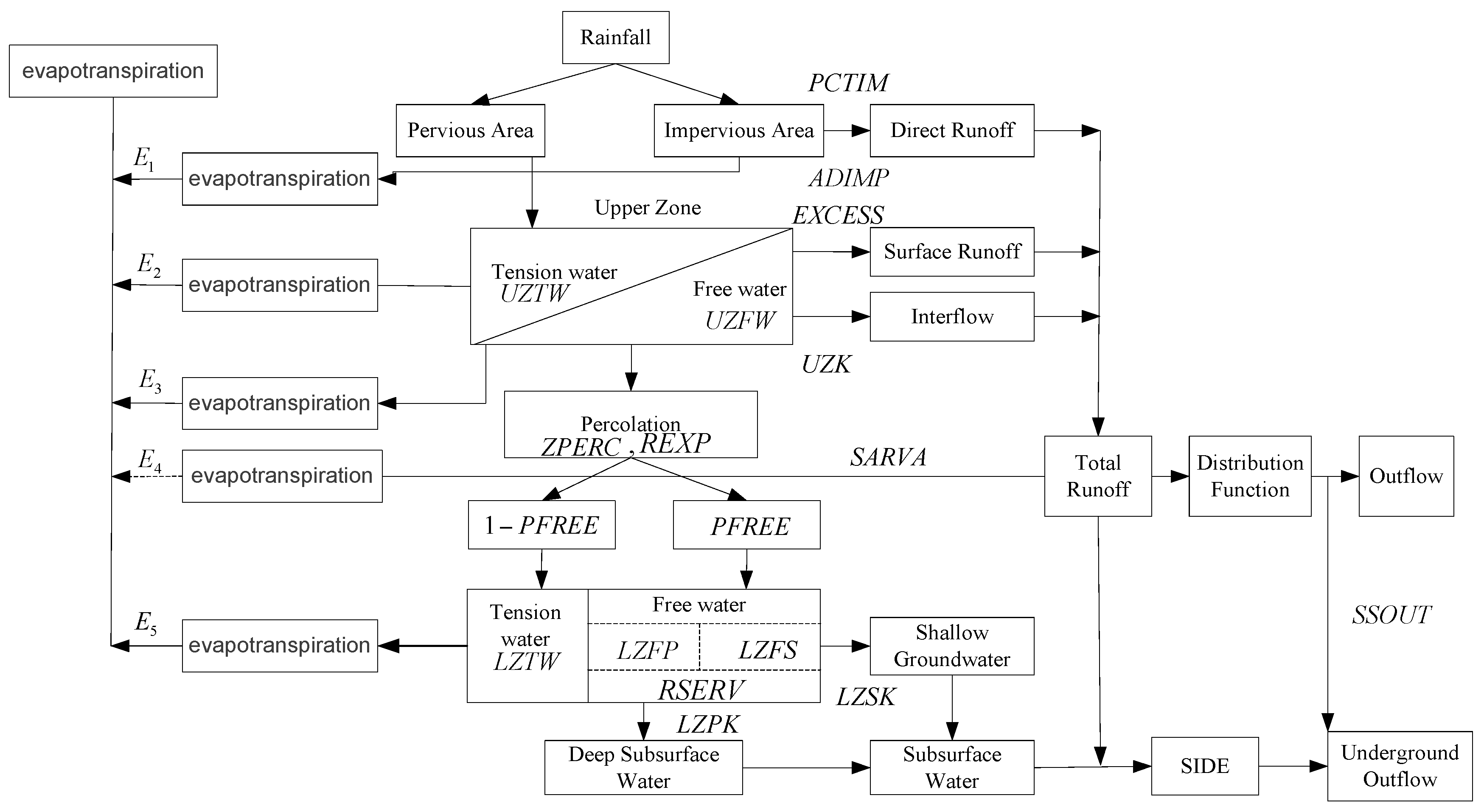
Figure 3.
Map of Dongyang river basin (left) and Tantou river basin (right).
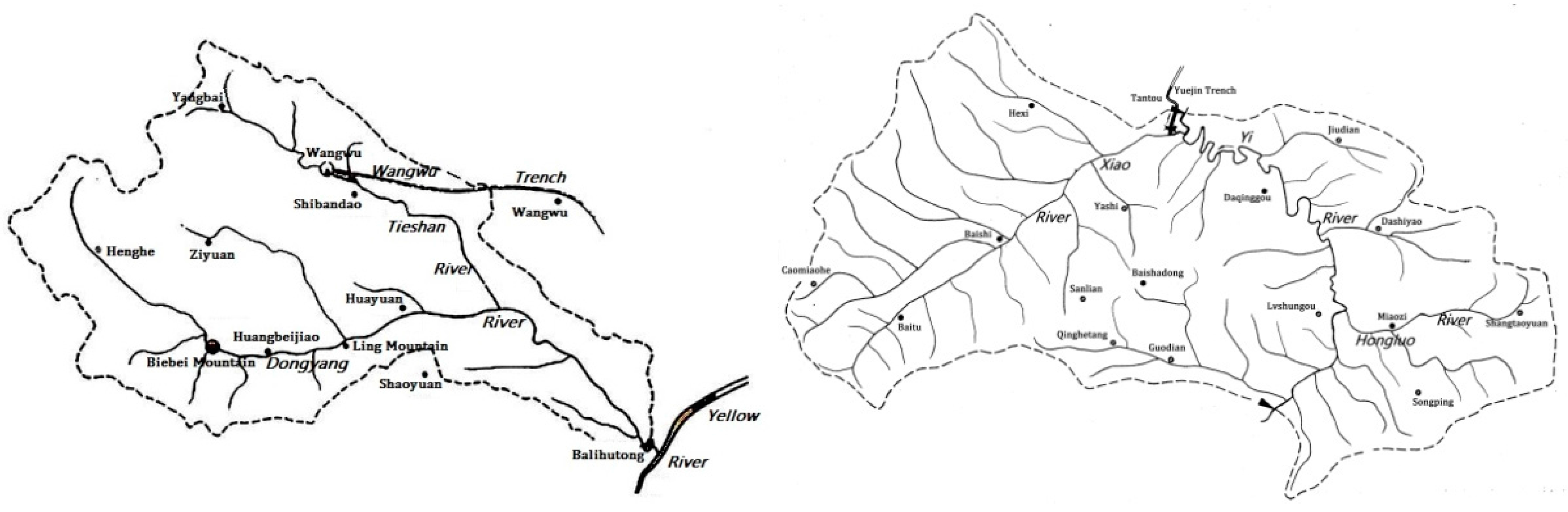
Figure 4.
The framework diagram of artificial ideal data generation.

Figure 5.
The parameter sensitivity analysis results based on the perturbation analysis method.

Figure 6.
The parameter sensitivity analysis results based on the GLUE method.

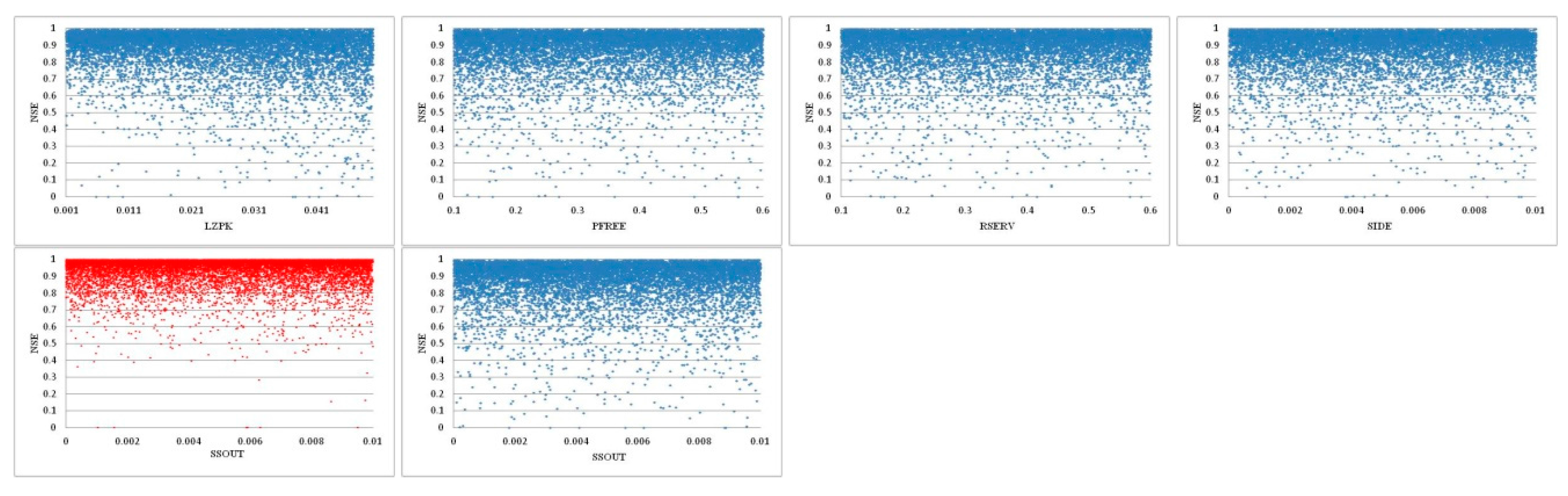
Figure 7.
The value of objective functions. (a) The objective functions of the flood in Tantou river basin. (b) The local enlarged figure of figure (a). (c) The objective functions of the flood in Dongyang river basin. (d) The local enlarged figure of figure (c).
Figure 7.
The value of objective functions. (a) The objective functions of the flood in Tantou river basin. (b) The local enlarged figure of figure (a). (c) The objective functions of the flood in Dongyang river basin. (d) The local enlarged figure of figure (c).

Figure 8.
The criteria comparison between the two methods of the two river basins. (a) The runoff absolute error comparison between the two methods of the two basins; (b) The runoff relative error comparison between the two methods of the two basins; (c) The peak flow absolute error comparison between the two methods of the two basins; (d) The peak flow relative error comparison between the two methods of the two basins; (e) The TRMS comparison between the two methods of the two basins; (f) The NSE comparison between the two methods of the two basins; (g) The %BIAS comparison between the two methods of the two basins.


Figure 9.
Simulation results comparison between single-step method and multi-step method. (a) The simulation results of No.870605 flood in Dongyang river basin. (b) The simulation results of No.880810 flood in Dongyang river basin. (c) The simulation results of No.880814 flood in Dongyang river basin. (d) The simulation results of No.870605 flood in Tantou river basin. (e) The simulation results of No.880706 flood in Tantou river basin. (f) The simulation results of No.880815 flood in Tantou river basin. (g) The simulation results of No.880818 flood in Tantou river basin. (h) The simulation results of No.890710 flood in Tantou river basin. (i) The simulation results of No.890716 flood in Tantou river basin. (j) The simulation results of No.890815 flood in Tantou river basin.

Table 1.
Value range and physical meaning of parameters in Sacramento model.
| Parameters | Physical Meanings | Maximum | Minimum |
|---|---|---|---|
| PCTIM | Permanent impervious area fraction | 0.05 | 0.01 |
| ADIMP | Maximum fraction of an additional impervious area due to saturation | 0.05 | 0.01 |
| SARVA | Area proportion of riverway, lakes and aquatic organisms | 0.05 | 0.01 |
| UZTWM | The upper layer tension water capacity, mm | 30 | 10 |
| UZFWM | The upper layer free water capacity, mm | 45 | 10 |
| UZK | Interflow depletion rate from the upper layer free water storage, day−1 | 0.7 | 0.2 |
| ZPERC | Ratio of maximum and minimum percolation rates | 25 | 5 |
| REXP | Shape parameter of the percolation curve | 3.0 | 1.4 |
| LZTWM | The lower layer tension water capacity, mm | 150 | 80 |
| LZFSM | The lower layer supplemental free water capacity, mm | 50 | 10 |
| LZFPM | The lower layer primary free water capacity, mm | 150 | 50 |
| LZSK | Depletion rate of the lower layer supplemental free water storage, day−1 | 0.3 | 0.01 |
| LZPK | Depletion rate of the lower layer primary free water storage, day−1 | 0.05 | 0.001 |
| PFREE | Percolation fraction that goes directly to the lower layer free water storages | 0.6 | 0.1 |
| RSERV | Fraction of lower layer free water not transferable to lower layer tension water | 0.6 | 0.1 |
| SIDE | Ratio of deep percolation from lower layer free water storages | 0.01 | 0.0 |
| SSOUT | The runoff loss factor in channel | 0.01 | 0.0 |
Table 2.
The comparison of four optimal algorithms in calibrating parameters.
| Parameter | Real Value | Flood No.820801 (Dongyang Basin) | Flood No.820730 (Tantou Basin) | ||||||
|---|---|---|---|---|---|---|---|---|---|
| SCE-UA | PGA | SMSE-PSO | ICSA | SCE-UA | PGA | SMSE-PSO | ICSA | ||
| PCTIM | 0.01 | 0.013 | 0.012 | 0.011 | 0.010 | 0.016 | 0.011 | 0.01 | 0.01 |
| ADIMP | 0.01 | 0.012 | 0.010 | 0.010 | 0.010 | 0.045 | 0.034 | 0.016 | 0.011 |
| SARVA | 0.01 | 0.009 | 0.01 | 0.009 | 0.01 | 0.012 | 0.015 | 0.014 | 0.012 |
| UZTWM | 20 | 19.34 | 20.01 | 19.95 | 20.03 | 18.92 | 18.64 | 19.50 | 19.79 |
| UZFWM | 20 | 19.67 | 19.88 | 20.03 | 20.01 | 17.84 | 18.92 | 19.42 | 19.98 |
| UZK | 0.4 | 0.398 | 0.395 | 0.397 | 0.399 | 0.417 | 0.405 | 0.402 | 0.398 |
| ZPERC | 16 | 16.01 | 16.01 | 15.99 | 15.98 | 15.48 | 15.67 | 16.04 | 16.00 |
| REXP | 2.0 | 2.01 | 2.0 | 1.98 | 2.01 | 2.16 | 1.98 | 1.99 | 1.99 |
| LZTWM | 100 | 100.6 | 100.4 | 99.98 | 99.99 | 98.31 | 99.50 | 99.60 | 100.1 |
| LZFSM | 40 | 39.56 | 39.68 | 39.94 | 39.98 | 38.74 | 39.51 | 39.42 | 39.8 |
| LZFPM | 100 | 100.56 | 100.32 | 100.26 | 100.03 | 103.8 | 102.4 | 98.1 | 100.3 |
| LZSK | 0.10 | 0.14 | 0.11 | 0.10 | 0.11 | 0.095 | 0.098 | 0.112 | 0.101 |
| LZPK | 0.005 | 0.005 | 0.005 | 0.005 | 0.005 | 0.004 | 0.005 | 0.005 | 0.005 |
| PFREE | 0.35 | 0.326 | 0.314 | 0.347 | 0.349 | 0.348 | 0.35 | 0.348 | 0.351 |
| RSERV | 0.3 | 0.301 | 0.299 | 0.302 | 0.300 | 0.312 | 0.301 | 0.298 | 0.301 |
| SIDE | 0.001 | 0.001 | 0.001 | 0.001 | 0.001 | 0.002 | 0.001 | 0.001 | 0.001 |
| SSOUT | 0.001 | 0.001 | 0.001 | 0.001 | 0.001 | 0.001 | 0.001 | 0.001 | 0.001 |
Table 3.
The comparison of performances of four optimal algorithms.
| River Basins | Flood No. | Algorithms | Time(s) | Iterations | Objective Functions | NSE |
|---|---|---|---|---|---|---|
| Dongyang | 820801 | SCE-UA | 13.01 | 136 | 14.1367 | 0.9997 |
| Dongyang | 820801 | PGA | 12.14 | 128 | 10.2681 | 0.9998 |
| Dongyang | 820801 | SMSE-PSO | 10.32 | 105 | 6.4891 | 1.0000 |
| Dongyang | 820801 | ICSA | 6.95 | 88 | 2.1943 | 1.0000 |
| Tantou | 820730 | SCE-UA | 16.23 | 143 | 17.8529 | 0.9997 |
| Tantou | 820730 | PGA | 14.57 | 134 | 14.7167 | 0.9997 |
| Tantou | 820730 | SMSE-PSO | 11.29 | 113 | 12.4674 | 0.9998 |
| Tantou | 820730 | ICSA | 8.24 | 99 | 8.4972 | 0.9999 |
Table 4.
Results of parameters estimation of single-step (shorten as single) and multi-step (shorten as multi) method.
Table 4.
Results of parameters estimation of single-step (shorten as single) and multi-step (shorten as multi) method.
| Parameters | Dongyang Basin | Tantou Basin | Parameters | Dongyang Basin | Tantou Basin | ||||
|---|---|---|---|---|---|---|---|---|---|
| Single-Step | Multi-Step | Single | Multi | Single | Multi | Single | Multi | ||
| PCTIM | 0.049 | 0.049 | 0.010 | 0.010 | LZFSM | 50.000 | 22.902 | 26.359 | 49.999 |
| ADIMP | 0.049 | 0.049 | 0.049 | 0.049 | LZFPM | 80.473 | 149.999 | 121.648 | 55.009 |
| SARVA | 0.011 | 0.049 | 0.026 | 0.013 | LZSK | 0.279 | 0.299 | 0.299 | 0.299 |
| UZTWM | 23.058 | 21.687 | 29.999 | 30.000 | LZPK | 0.001 | 0.049 | 0.049 | 0.001 |
| UZFWM | 45.000 | 44.878 | 27.161 | 35.578 | PFREE | 0.100 | 0.599 | 0.431 | 0.100 |
| UZK | 0.200 | 0.200 | 0.248 | 0.240 | RSERV | 0.100 | 0.584 | 0.166 | 0.600 |
| ZPERC | 25.000 | 24.944 | 12.738 | 5.000 | SIDE | 0.009 | 0.000 | 0.000 | 0.010 |
| REXP | 1.400 | 1.400 | 2.999 | 3.000 | SSOUT | 0.000 | 0.003 | 0.010 | 0.010 |
| LZTWM | 149.99 | 127.259 | 117.368 | 149.999 | - | - | - | - | - |
© 2017 by the authors. Licensee MDPI, Basel, Switzerland. This article is an open access article distributed under the terms and conditions of the Creative Commons Attribution (CC BY) license (http://creativecommons.org/licenses/by/4.0/).
Share and Cite
MDPI and ACS Style
Zhang, G.; Xie, T.; Zhang, L.; Hua, X.; Liu, F. Application of Multi-Step Parameter Estimation Method Based on Optimization Algorithm in Sacramento Model. Water 2017, 9, 495. https://doi.org/10.3390/w9070495
AMA Style
Zhang G, Xie T, Zhang L, Hua X, Liu F. Application of Multi-Step Parameter Estimation Method Based on Optimization Algorithm in Sacramento Model. Water. 2017; 9(7):495. https://doi.org/10.3390/w9070495
Chicago/Turabian StyleZhang, Gang, Tuo Xie, Lei Zhang, Xia Hua, and Fuchao Liu. 2017. "Application of Multi-Step Parameter Estimation Method Based on Optimization Algorithm in Sacramento Model" Water 9, no. 7: 495. https://doi.org/10.3390/w9070495
Note that from the first issue of 2016, this journal uses article numbers instead of page numbers. See further details here.