Sediment Size Effects in Acoustic Doppler Velocimeter-Derived Estimates of Suspended Sediment Concentration

Department of Civil Engineering, Yildiz Technical University, Istanbul 34220, Turkey
Water 2017, 9(7), 529; https://doi.org/10.3390/w9070529
Submission received: 16 June 2017
/
Revised: 11 July 2017
/
Accepted: 11 July 2017
/
Published: 16 July 2017
Abstract
:Backscatter output from a 10 MHz acoustic Doppler velocimeter (ADV) was used to quantify suspended sediment concentrations in a laboratory setting using sand-sized particles. The experiments included (a) well-sorted sand samples ranging in size from 0.112 to 0.420 mm, obtained by the sieving of construction sand, (b) different, known mixtures of these well-sorted fractions, and (c) sieved natural beach sand with median sizes ranging from 0.112 to 0.325 mm. The tested concentrations ranged from 25 to 3000 mg·L−1. The backscatter output was empirically related to concentration and sediment size, and when non-dimensionalized by acoustic wavelength, a dimensionless sediment size gradation coefficient. Size-dependent upper and lower bounds on measurable concentrations were also established empirically. The range of measurable conditions is broad enough to make the approach useful for sand sizes and concentrations commonly encountered in nature. A new method is proposed to determine concentrations in cases of mixed-size sediment suspensions when only calibration data for well-sorted constituent sands are available. This approach could potentially allow better estimates when the suspended load is derived from but is not fully representative of the bed material, and when the size characteristics of the suspended material are varying in time over the period of interest. Differences in results between the construction and beach sands suggest that sediment shape may also need to be considered, and point to the importance of calibrating to sediments encountered at the site of interest.
1. Introduction
The transport of suspended sediment is an important issue in many problems related to agriculture, environment, and engineering [1,2,3]. The service life of engineered facilities such as dams and navigation channels, irrigation canals, and the health of ecosystems (marshes, deltas, estuaries) are all influenced by sedimentation and sediment transport [4,5]. In some environments and events, sediment kept in suspension by hydrodynamic processes accounts for the majority of the sediment transported past a location of interest. Both sands and finer material may be transported in suspension, depending on the magnitude of the energy in the flow, among other factors.
Most commonly, the quantification of suspended sediment concentration (SSC) has been done in one of two ways, classified here as direct and surrogate methods. Direct methods, employing water sampling bottles or submersible pumps, tend to be labor-intensive and in some cases not representative due to the spatial and temporal variability of the suspended sediment concentration in the water column. The main advantages of the direct method are its simplicity and the resulting availability of information on sediment characteristics, such as the shape, size, and mineralogy [6,7,8,9]. However, direct measurements of SSC or transport tend to be difficult to achieve with accuracy, particularly when frequent automated measurements are desired.
Surrogate methods are those that can be used to estimate suspended sediment concentration indirectly. Acoustic backscatter, optical backscatter sensors, and laser diffraction methods have all been employed. None of these methods involve the collection of water samples; they can thus be implemented autonomously without the need for any pumping or sampling bottles. They make possible nominally non-intrusive measurements with high temporal resolution. In some cases, the spatial variation in concentration might also be quantifiable. Methods employing acoustic signals tend to be less problematic logistically, as optical sensors are typically much more sensitive to biofouling in natural environments [10,11,12,13]. Multi-frequency acoustic sensors also have the potential to provide information on the size distribution of the suspended sediment.
Output from optical turbidity sensors is now routinely used to provide surrogate estimates of suspended sediment concentration. At most sites, turbidity and suspended sediment concentration are closely correlated, and often vary linearly. Direct measurements of suspended sediment concentrations are collected simultaneously with turbidity sensor output, and a calibration curve is developed that allows for the estimation of SSC directly from the measured turbidity [14,15,16].
Turbidity sensors can in general be classified into two groups: transmissometers and nephelometers. Transmissometers employ a light source beamed directly at a sensor, and measure the light transmission. Nephelometers measure light scattered by suspended particles rather than direct light transmissions. An optical backscatter sensor (OBS) is a type of nephelometer designed to measure backscattered infrared radiation from a small sampling volume, on the order of a few cm3 [17,18,19]. Each of these examples results in single point measurements, and all can be severely impacted by biofouling. Both transmittance and scatterance are functions of the number, size, index of refraction, and shape of suspended particles.
Optical instruments lack moving parts and provide rapid sampling capability compared to direct methods. The instruments rely on empirical calibrations to convert measurements to estimates of turbidity, which in turn is typically converted to a suspended sediment concentration via an additional empirical relationship. The relatively mature technology incorporated into these instruments typically provides reliable data; this approach is used routinely, for example, at a number of United States Geological Survey (USGS) streamgaging stations [14,20,21,22]. The maximum measurable concentration for these instruments depends in part on particle size distributions. The OBS has a generally linear response at concentrations of less than about 2000 mg·L−1 for clay and silt, and 10,000 mg·L−1 for sand [23].
Laser diffraction instruments have been used in the laboratory for several decades to measure volumetric particle concentration and particle size distribution. Field-deployable laser diffraction instruments have been used in many different water environments [24,25]. Laser diffraction measurements of concentration and particle size distribution are feasible over a limited range of sizes (2–380 microns). Measured light scattering from particles outside of these measurement size limits introduces errors, while particle shape and uncertainty or variability in sediment density influence the conversion from volumetric to mass concentration [26].
Acoustic Doppler current meters (including acoustic Doppler current profilers (ADCPs), acoustic Doppler profilers (ADPs), and acoustic Doppler velocimeters (ADVs)) are the most commonly used acoustic devices. They use the measured shift in the apparent frequency of transmitted sound waves to compute a three-dimensional (3-D) flow velocity. The strength of the acoustic return signal has also been used as a proxy for sediment concentration in water systems [17,27,28,29,30,31]. The basic principle for the measurement of suspended sediments is that acoustic waves passing through a water–sediment mixture will scatter and attenuate as a function of sediment, fluid, and instrument characteristics. The acoustic metrics of backscatter and attenuation are influenced by a sediment’s characteristics (primarily size and shape) and concentration within an ensonified volume. Compensation is typically introduced to account for the influence of fluid and instrument characteristics, either theoretically or empirically.
ADVs are nominally single-point measurement devices, yielding velocity estimates for a small (O(0.1 cm3)) sampling volume, typically 5–10 cm away from the instrument. Acoustic profiling instruments (i.e., ADCPs and ADPs) employ range-gating of the reflected sound signal to resolve the spatial variations in their along-beam velocities, which can then be converted to velocity profiles in a Cartesian coordinate system (Figure 1). Profiling instruments have a distinct advantage over most other surrogate technologies in that they can provide data indicative of conditions spanning a substantial section of a river cross-section or water column.
Several researchers have investigated the performance of acoustic Doppler current profilers for the prediction of SSC in various water environments, including coastal environments and rivers [32,33,34,35,36]. Predictions are derived by empirically relating device output (typically acoustic signal-to-noise ratio or return signal amplitude in counts or decibels) and the SSC of the water [37,38,39,40,41,42]. When an acoustic instrument is calibrated for a water system in which suspended sediment properties display little time dependence, no additional sensor is needed to measure the SSC. This approach then provides simultaneous measurements of velocity and concentration via one acoustic sensor that is typically much less susceptible to errors due to biofouling than with optical sensors. However, the calibration makes the acoustic approach highly site-specific and in some cases strongly seasonally dependent, due to the sensitivity of the acoustic response to the particle size, density, shape, and composition of scatterers in the target volume.
The new work described here was intended to investigate the sensitivity of the acoustic estimates of suspended sediment concentration to sediment size and size distribution. A point-measurement acoustic Doppler velocimeter (ADV) was used in a controlled laboratory environment so that the suspended sediment concentration was readily controlled and known. Tests were done both with the original sediment mixture and with well-sorted fractions obtained by sieving the mixture. Both construction sand and marine beach sand were considered. A description of the experimental methodology, results, and conclusions follow.
2. Materials and Methods
2.1. Instrumentation and Theoretical Background
An acoustic Doppler velocimeter (ADV) is attractive for measuring instantaneous velocities, given that it features a measurement volume somewhat remote from the instrument, and can output results at frequencies suitable for the measurement of turbulence with a relatively small (O(0.1 cm3)) sampling volume [43,44,45,46]. Although developed to measure water velocities, over the past few decades several studies have demonstrated the successful implementation of these devices to estimate SSC in the field and in the lab [40,41].
Here, a 10 MHz Nortek Vectrino acoustic Doppler velocimeter was used for measuring SSC in a laboratory setting. The claimed performance characteristics of the device are as follows: acoustic frequency 10 MHz; velocity range ±0.03, 0.10, 0.30, 1.0, 2.5, or 4 m/s (user-selectable); velocity resolution 0.1 mm/s; velocity bias ±0.5% with no measurable zero-offset in the horizontal direction; sampling (output) rate between 0.1 and 25 Hz; random noise corresponding to approximately 1% of the range at a 25 Hz sampling rate; diameter and height of the cylindrical measurement volume are 6 and 7 mm, respectively, corresponding to a volume of ≈0.20 cm3; minimum distance from the sampling volume to a physical boundary 5 mm [47].
The ADV transmits short-duration acoustic pulses along its transmit beam. As the pulses propagate through the water, a fraction of the acoustic energy is absorbed by both the water and scatterers suspended in the water (e.g., suspended sediments, small organisms, etc.). The rest of the energy either continues propagating or is scattered back and detected by a receiver. The amount of absorbed and reflected energy depends on the fluid’s properties (e.g., temperature, salinity, pressure, etc.), the scatterer’s properties (density, shape, and diameter), the concentration, and the measurement device’s acoustic frequency and power.
In contrast to flow velocity measurements, where the frequency shift of backscattered sound is post-processed to determine three-dimensional velocity information, here the strength of the reverberated sound is analyzed. The relationship between SSC and the so-called relative acoustic backscatter (RB) can be expressed as [47]:
The parameters A and B in Equation (1) are empirical and can be derived from known SSC and RB data pairs using least squares fitting. The relative backscatter is the measured acoustic backscatter corrected for transmission losses in units of either decibels (dB) or counts. Typically, a proportion is assumed between count and decibel. The ADV used in this study, counts, is multiplied by 0.43 to convert to decibels, per the manufacturer’s recommendations. Following [48], RB can be computed as:
where RL is the reverberation level (the measured backscatter intensity of the received signal), and 2⋅TL is the estimated two-way transmission loss, assumed to be the same in each direction. RL can be taken as the actual reported values or the reported values minus the noise level as it was applied in this study. If the noise level is relatively constant, there is negligible difference between the two approaches.
RB = RL + 2⋅TL
SSC is typically measured either via direct methods or via a different indirect method, such as with an optical turbidity sensor. The study described here involved introducing a known mass of sediment into a known volume of water in the laboratory, and agitating to establish a uniform concentration, so the concentration was well known.
The term ‘transmission loss’ consists of losses accounted for by the spherical spreading of the beam (first term on the right hand side of Equation (3)) and losses due to absorption (second term):
where R is the along-beam range from the transducer’s head to the measurement location (m). This loss can be significant for profiling instruments, where the range may be tens of meters, but is much less significant with point measurement devices, where the range is typically on the order of 10 cm, and is 10 cm in this study. Here, is called the near-field correction factor, and has to be introduced when calculating the effect of spherical spreading close to the transducer [49]. The coefficient α describes the absorption of energy by water () and attenuation due to suspended sediments (), i.e., (all in dB/m). Spatial variations in suspended sediment concentration would imply a similar variability in , but data to define this variability is rarely available a priori.
The coefficient is a function of sound frequency, salinity, temperature, and pressure. However, pressure does not have a significant effect on the absorption coefficient for shallow water environments (depth ≤ 20 m) [37]. Several equations have been proposed for estimating [50,51]. In the present study, was calculated as follows [51]:
where f is the instrument frequency (Hz), and T is the water temperature in °C. Attenuation due to the suspended load is dependent on scattering and viscous absorption by the suspended material. Viscous losses are primarily due to the concentration of finer particles, while scattering losses are primarily attributable to the coarser particles [30]. Here, was calculated for each experiment using Equation (5). This approach was proposed by Crawford and Hay [10] as a modification of Urick’s (1948) Equation [52]:
where SSCV is the volumetric sediment concentration (SSC divided by sediment density), k is the wave number, 2π/λ, in which λ is the acoustic wavelength in cm, γ is the specific gravity of sediment, here 2650 kg/m3, is the mean sediment radius in cm, s is equal to , τ is equal to [ω/2υ]5, ω is 2πf, f is frequency in Hz, υ is the kinematic viscosity of water, in stokes, and the constant is required for the conversion from nepers/m to dB/m. The first term within the brackets is the acoustic attenuation due to viscous losses, and the second is the acoustic attenuation due to scattering losses.
Acoustic instrument response varies by the size of the suspended particles. Each acoustic frequency has a particle size for which it possesses peak sensitivity and a minimum detectable particle diameter. Theoretically, the best results are obtained when D/2 × k = 1, i.e., the circumference of the particle is equal to λ, where D is the diameter of particle, and k is the wavenumber [53]. For the instrument used in this study, the corresponding wavelength λ is equal to 0.14 mm and the greatest sensitivity is expected for a particle diameter close to 0.045 mm, which is finer than the finest sieve used to sort the sediment used in the experiments.
2.2. Backscatter vs. Concentration
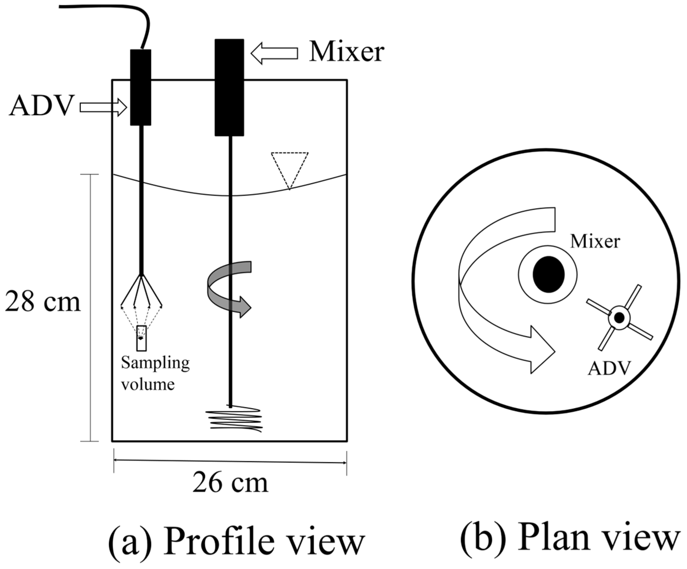
A series of laboratory experiments was designed to investigate the relationship between suspended sediment concentration, sediment size and size distribution, and acoustic backscatter, using a 10 MHz Nortek acoustic Doppler velocimeter. The experiments were conducted in a laboratory using a simple set-up seen in Figure 2. A similar experimental apparatus was previously used in the lab successfully by the researchers studying on the subject, and it was shown that the set-up is capable of creating a high-level uniform suspension in the container [54,55]. An estimated maximum error of 0.5 cm in these dimensions translates to a maximum 1.8% error in water volume. All of the experiments were done with sand, and sand mass was measured to the nearest mg. The computed suspended sediment concentrations are thus known within 2%.
Construction sand was used for most of the experiments. The sand was sieved to yield fractions with median sizes of 0.420, 0.325, 0.215, 0.165, and 0.112 mm. Some experiments made use of mixtures created by re-combining different size fractions in different proportions; others were performed on specific size fractions resulting from sieving and will be referred to as “well-sorted” hereafter. A total of 56 experiments were performed, with different mean grain sizes and at different concentrations (Table 1). For a given mass concentration, backscatter and size are inversely related. For any size, as the concentration increases, acoustic saturation eventually occurs; however, with the finer sediments, this occurs earlier. This explains why Table 1 shows fewer experiments with the finer sediments than with the larger sizes.
A helical mixer mounted in a drill was inserted vertically in the center of the bucket and operated at a fixed torque to yield a uniform sediment suspension in the cylindrical tank. This was verified by repeated measurements (six trials per concentration and mixture, each lasting 60 s after spin-up). Figure 3 shows two examples of the dependence of backscatter amplitude (raw) vs. concentration: one case with well-sorted sand with a mean diameter of 0.165 mm, and the other with mixed-sand with a mean diameter of 0.295 mm. Each plotted result incorporates all six measurements for that particular scenario. The central mark is the median amplitude, the edges of each box are the 25th and 75th percentiles, and the whiskers extend to the most extreme data points. The approach to acoustic saturation is seen in both plots, with this point arriving at a lower concentration in the case of the finer sediment.
The acoustic noise reported by the instrument was fairly consistent. It was not subtracted from the amplitudes plotted in Figure 3, but it was removed from the raw backscatter amplitudes for all further analysis and plots. The transmission losses were estimated using Equations (3)–(5), but were found to be negligible. As a result, the relative backscatter RB in Equation (2) was taken as RB = RL − Noise. Given that Equation (1) is empirical and noise levels varied little between experiments, the subtraction of the noise from the reported backscatter amplitude is not a critical step, but seems appropriate to allow for any cases which for whatever reason have increased noise levels.
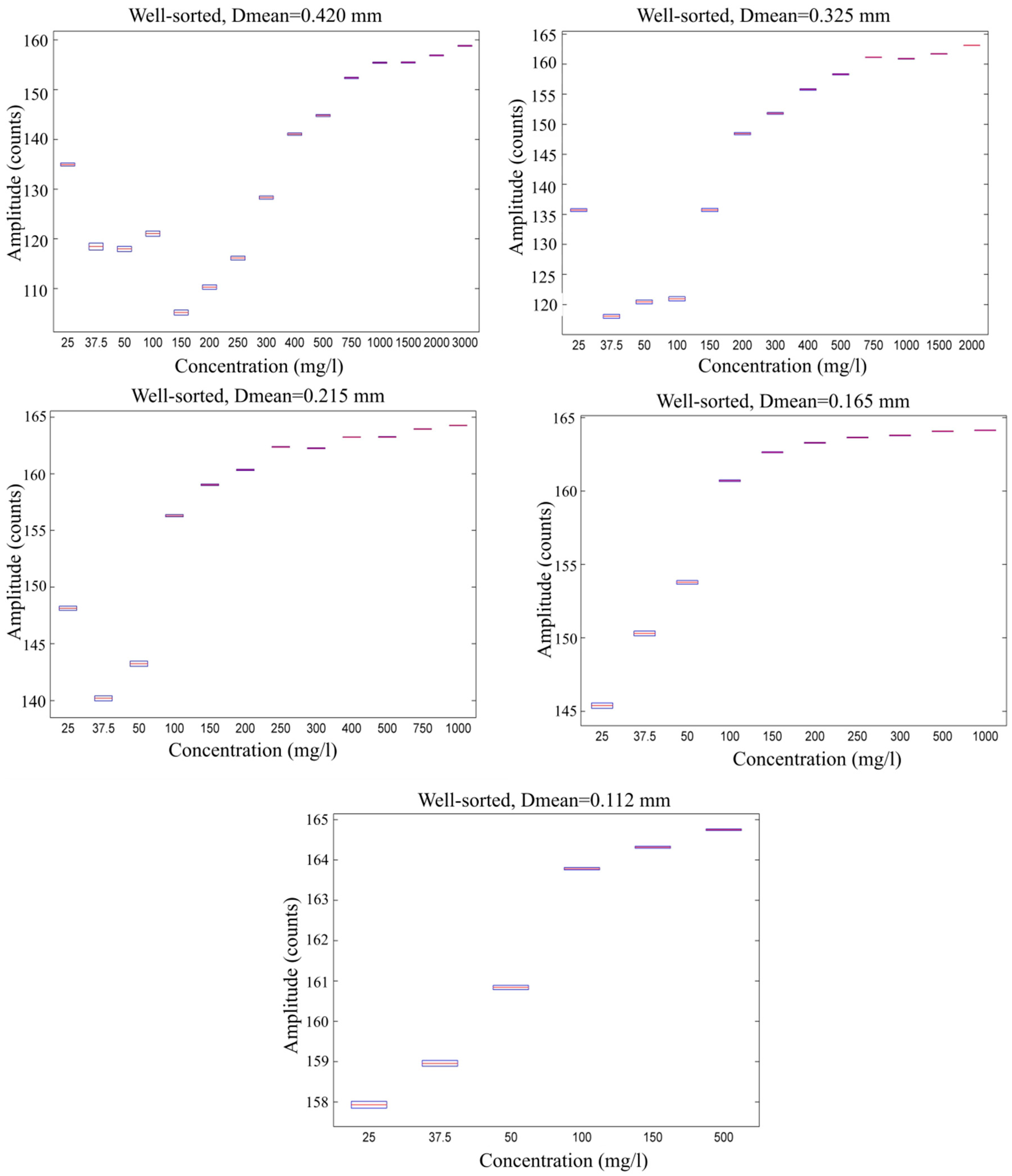
Figure 3 reveals that there is a size-dependent upper bound on the suspended sediment concentration that can be correlated with the backscatter. Figure 4 shows the results for five different size fractions and a larger range of concentrations, revealing that there is also a size-dependent lower bound on concentration where the relationship to backscatter changes. The problem is evident in the first three panels of Figure 4, which correspond to larger sediment sizes. With coarse sand at low concentrations in a very small sampling volume, the presence or absence of a few grains of sediment can lead to a significant change in concentration in the sampling volume. For the largest sand size tested, at the lowest concentration, the number of sand grains present in the sampling volume, on average, is 0.2, implying that most of the time, there is no sand grain inside the sampling volume. Because of the uncertainty that appears at these low concentrations, only the portions of the curves shown in Figure 4, where backscatter increases monotonically with concentration, were considered for further analysis.
The relations between the lowest and highest measurable SSC and non-dimensional median diameter, D/λ, were established empirically. The minimum measurable concentration for each tested size fraction was defined as the lowest concentration above which backscatter increased monotonically with concentration. A best-fit linear relationship was determined between this lower-bound concentration and dimensionless sediment size. A similar approach was used to develop a relationship between maximum measurable concentration and sediment size. At high concentrations, the backscatter approaches a constant value. The point at which an increase in concentration resulted in no more than a one count increase in backscatter was defined as the maximum measurable concentration. The two resulting relationships are given by Equation (6):
These are empirical relationships; thus it is important to remember that they should not be applied outside of the tested ranges, i.e., sediment size 0.112 to 0.420 mm.
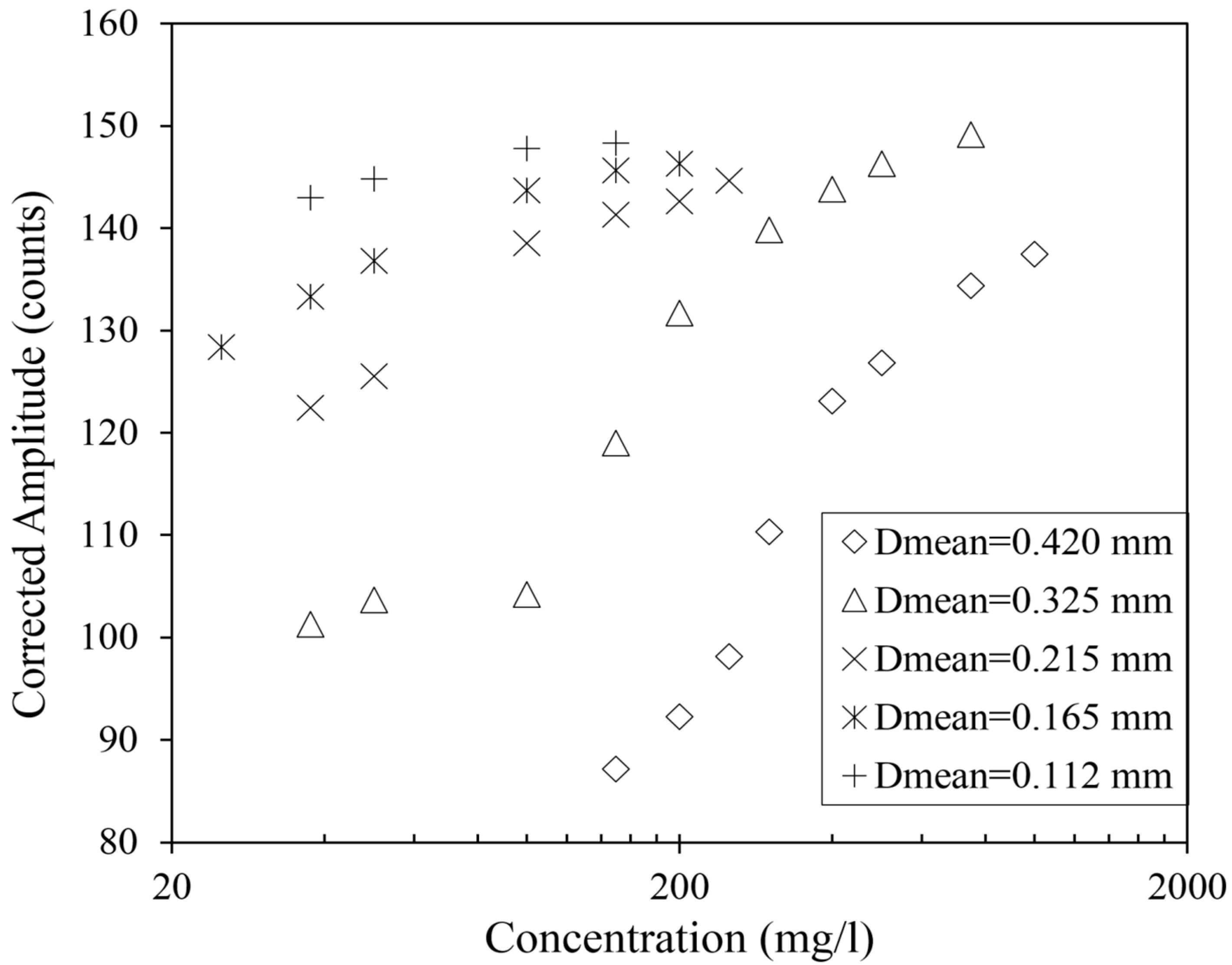
Figure 5 shows corrected amplitude (raw amplitude minus reported noise level) vs. concentration for the well-sorted cases considered for further analysis. Only the points lying between the minimum and maximum measurable concentrations are shown.
A second group of experiments was performed using different mixtures of the same sieved sediments. Five different mixtures were created, and 70 experiments performed with these mixtures, with concentrations ranging from 20 mg/L to over 200 mg/L, at increments of 20 mg/L (Table 2). In this table, Dmean is the mean diameter of the sediment populations, and Cg is a dimensionless coefficient of gradation. Different definitions of this coefficient are available; here it is taken as D90/D10, where D90 and D10 denote the particle diameters such that 90% and 10% of the mixture are finer, respectively, by weight.
The sediment mixtures featured different upper limits on measurable concentration compared to the well-sorted cases. Equation (7) for the upper bound was derived in the same manner as Equation (6), but for the mixed sand cases. There was, however, no need to derive a new relation for the lower bound on measurable concentration.
The calculated upper bounds for the sediment mixtures shown in Table 2 vary from 160 to 200 mg∙L−1.
3. Results
Equation (1), presented above, has been used by others to predict the suspended sediment concentration from relative or corrected backscatter readings. It is empirical in nature, and requires calibration for the conditions of interest. It does not (explicitly) include the sediment’s size or size distribution, although results shown so far clearly reveal that sediment size characteristics are important.
A dimensional analysis and theoretical considerations suggest that the ratio of the representative particle diameter to the acoustic wavelength is appropriate to incorporate the influence of particle size. With this parameter and the coefficient of gradation introduced, the dimensional analysis problem may be stated as:
where is sediment density, RB is relative backscatter intensity, D is a representative grain size, and is the acoustic wavelength. The wavelength was effectively constant in the experiments, but the ratio of sediment size to wavelength varied. Sediment density was assumed to be constant.
A series of empirical relationships was tested to determine the functional relationship between the four parameters listed in Equation (8). In each case, it was assumed that the log of SSC was the appropriate dependent variable, but some of the options tested included nonlinear dependence on the corrected backscatter amplitude and dimensionless sediment size. Nonlinear least squares regression was used to determine the coefficients providing the best fit to the data.
Three sets of experimental results were available for consideration: tests conducted with (1) sieved construction sand, referred to as well-sorted, (2) well-sorted construction sand mixed together in known proportions, referred to as mixed, and (3) natural beach sand from Folly Island, South Carolina, also sieved to yield well-sorted fractions. Each will be considered below in sequence. In each case, the speed of the sound reported by the instrument (based on the measured temperature) was used to compute the acoustic wavelength, assuming a frequency of 10 MHz. The coefficient of gradation was omitted from the regression process for the well-sorted cases. The well-sorted sediments are not truly uniform in size, but their coefficients of gradation are much smaller than for the mixed sediments (and unknown), and should vary little between cases, making it impossible to see the influence of gradation.
Nonlinear regression was used to determine best-fit coefficients for three different equations consistent with Equation (8), using the experimental data from the well-sorted sand tests, with omitted for these cases. The first two formulations assumed linear dependence on the corrected amplitude and sediment size; the last allowed nonlinear dependence on these parameters. In each case, the dimensionless root-mean-square error, denoted here as RMSE, was used to quantify the goodness-of-fit between the known and predicted concentrations:
where SSCki is the ith known value of SSC, and SSCpi is the ith predicted value. Thirty-three cases with well-sorted sand of different sizes and different concentrations were evaluated.
The three equations and the resulting dimensionless RMS errors are given by Equations (10)–(12):
The results obtained using each of these three equations can be seen in Figure 6. Equation (12), having two additional adjustable parameters in the form of exponents, unsurprisingly yields the lowest error, but the simpler form of Equation (11) is preferable and still yields similar results. Note that the exponents on amplitude and dimensionless grain size are both O(1); neither input variable is negligible.
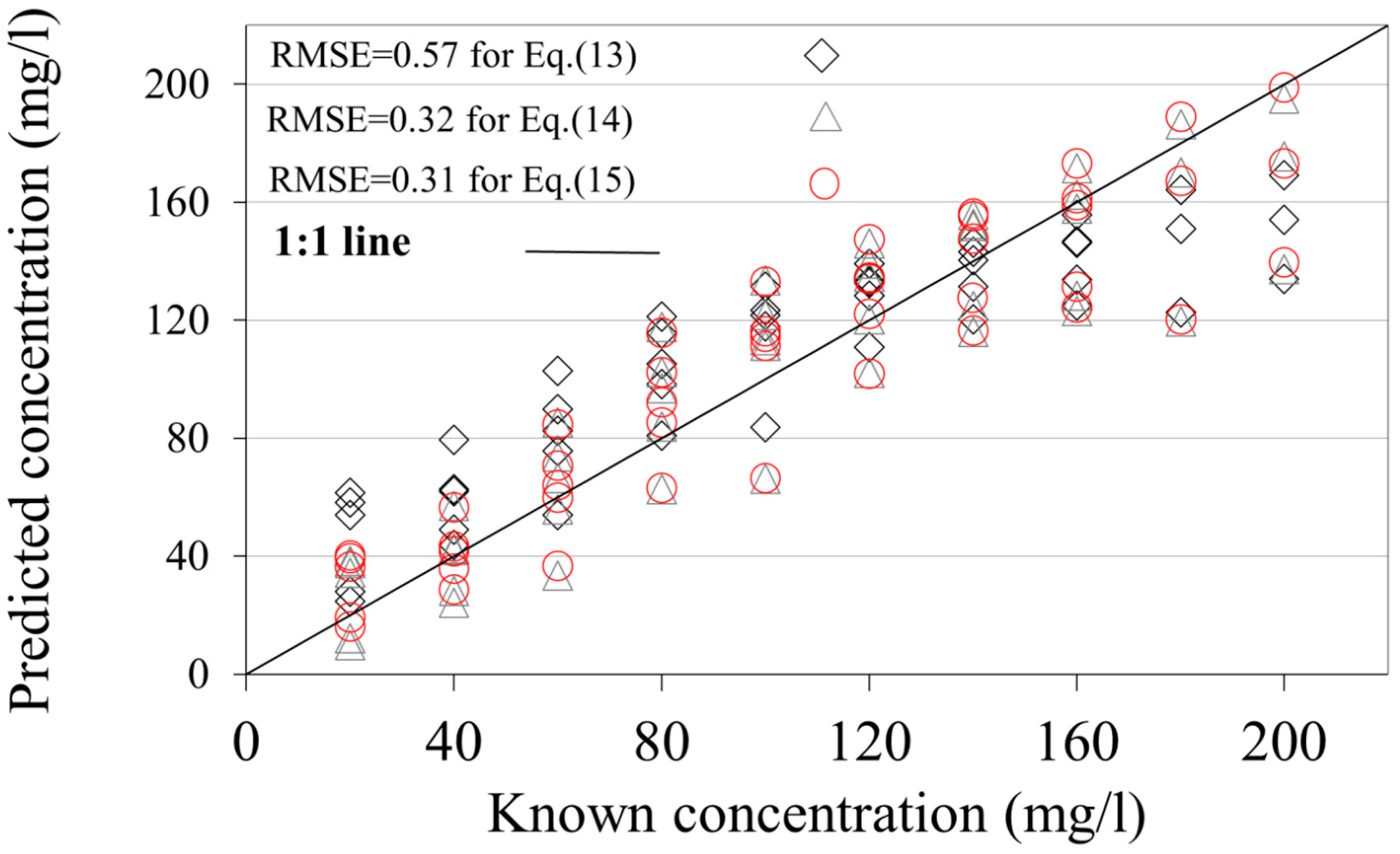
The five different sand mixtures (Table 2) resulted in mean diameters of 0.208–0.295 mm, with coefficients of gradation of 2.8–6.3. Nonlinear regression was performed on the dataset obtained with these sediments, as described above, but this time with the coefficient of gradation included as one of the independent variables. Equations (13)–(15) are the resulting best-fit formulations:
The results obtained with Equations (13)–(15) are shown in Figure 7. The results are similar for all three formulations, so the simpler form represented by (14) is preferable. Together, these results suggest that SSC predictions should be based on the first power of corrected backscatter amplitude, relative diameter, and coefficient of gradation. The results are weakly dependent on the coefficient of gradation, as revealed by each of Equations (13)–(15).
Attempts were then made to predict the concentrations for the mixed sediments based solely on the results for the individual size fractions that made up each mixture. One method tested was linear superposition of the best-fit empirical coefficients obtained for the well-sorted sediments, weighted by the respective abundances by size class. Note that Equation (11) has the general form of log(SSC) = A × Amp + B × Size + C. For each of the ith sediment sizes, Equation (11) was applied to the available data to determine best-fit values Ai, Bi, and Ci. The resulting values for each mixture were then computed as
where pi denotes the fraction of the ith size class in the mixture. This resulted in a slight improvement when predicting results for mixed sand, compared to using Equation (11) directly, but the different size classes do not contribute equally to the backscatter signal, even if present in the same proportions, as revealed earlier by Figure 5, for example. Therefore, a different weighting scheme was invoked:
A linear, best-fit approach was applied to determine the relationship between the three new weighting coefficients (α, β, and γ) and Cg. An inverse relation between and Cg resulted, whereas the other two coefficients were constant.
Equation (18) shows that B = 0 provides the best fit, suggesting that the dimensionless sediment size is not relevant to predicting the concentration from the backscatter for the mixed sand cases. It should be noted, however, that the median grain size for the mixed sand cases varied much less than for the well-sorted cases. A wider range of median sizes would be expected to yield a result other than B = 0.
Using the approach summarized above, the coefficients A and C were calculated for each mixture in Table 2 and applied using Equation (14). The resulting RMS errors are 0.54 for Mix I, 0.50 for Mix II, 0.76 for Mix III, 0.72 for Mix IV, and 0.62 for Mix V. The agreement with the measurements is thus not as close as obtained using Equation (14) with the well-sorted sediments, where the RMS error was 0.32. But this new method represents a means of predicting concentration from calibration data obtained only for the various size fractions within a mixture. For a scenario where sediments are being lifted from the bed in time-dependent proportions, due to changes in flow characteristics, the grain size distribution will vary continuously as flow conditions change. If one can predict which sizes are traveling in suspension at any given time, and in what proportions, or measure this independently, this method could be used to estimate concentration from backscatter data.
The last set of tests made use of natural beach sand from Folly Island, South Carolina, sieved to yield well-sorted fractions. The properties of the sediment fractions and the experimental conditions are summarized in Table 3. Applying Equations (10)–(12) without recalibration to this dataset resulted in RMS errors of 0.62, 0.62, and 0.51, comparable to when they were applied to the tests with the well-sorted construction sand.
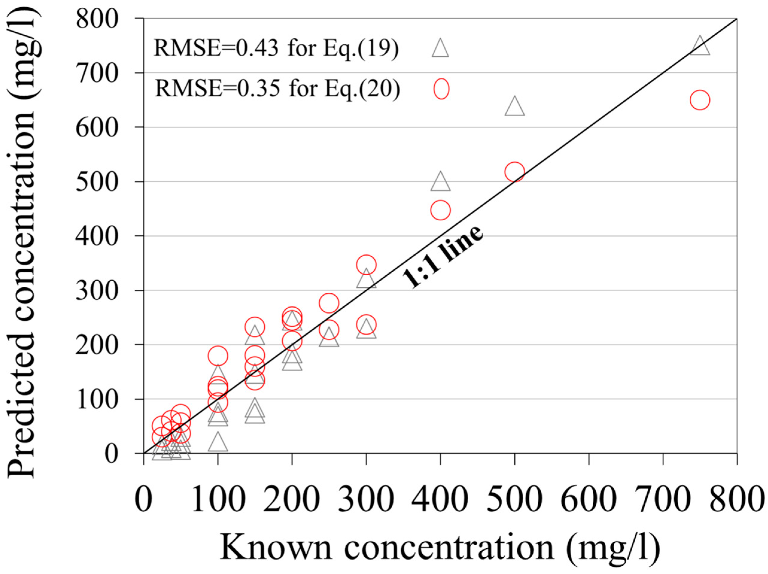
Repeating the regression process assuming the same form as Equations (11) and (12), to determine best-fit coefficients for the Folly Island sand, yielded Equations (19) and (20):
The resulting predicted and measured suspended sediment concentrations are shown in Figure 8. Equation (19) is preferred because it yields results nearly as good as those obtained using Equation (20), with fewer adjustable parameters.
Equations (11) and (19) have the same form and both represent best fits to well-sorted sediment fractions of similar sizes. One may question the suitability of the proposed form of the equation if different sediments require different best-fit coefficients. It is possible that another parameter, not measured or included, such as sediment shape, plays a role. The verification of this hypothesis would require additional investigation.
4. Discussion and Conclusions
A series of laboratory experiments was performed with fine- and medium-sized sand to investigate the feasibility of estimating suspended sediment concentration using the backscatter signal from an acoustic Doppler velocimeter. Particular emphasis was placed on the influence of sediment size and size distribution on the problem. Three sets of experiments were conducted, using (1) well-sorted sands obtained by sieving construction sand, (2) well-sorted sands obtained by sieving marine beach sands, and (3) different combinations of the well-sorted construction sands to mimic more natural size distributions. The suspended sediment concentration was adjusted systematically with each sediment size to provide a dataset spanning a range of concentrations and sediment sizes. Each experiment was conducted six times to allow quantification of repeatability and variability.
A dimensional analysis suggests that suspended sediment concentration should be predictable based on knowledge of the relative backscatter intensity, dimensionless grain size, and grain size distribution. Several relationships among these variables were tested to reveal the most suitable form. The results suggest that for well-sorted sediments, the log of the concentration is a linear function of both backscatter amplitude and size. Allowing the exponents on these terms to be variable results in nonlinear best-fit equations with only marginal improvements in RMS error values.
In natural aquatic environments, sediments are often poorly sorted. Tests with well-mixed sediments revealed that the basic form of the relationship between backscatter and size is unchanged, but the best-fit coefficients change. Including the coefficient of gradation in the equation relating backscatter to suspended sediment concentration does improve performance.
In many applications of acoustic to introduce a predicted equation for estimating SSC in any given water environment, the sediment that is in suspension is often assumed to be represented in the bed below, which is not wrong in certain aspects. However, this is not fully representative, as the finer material is more easily mobilized, which is why the median grain size of the material in suspension will often be smaller than that of the bed. Additionally, the median size of the material in suspension may be time-dependent, changing as flow energy increases or decreases, and influencing the flow’s transport capacity. Thus, there is an infinite number of possible grain size distributions for the suspended flow, even with a constant size distribution for the bed.
It is not possible to calibrate equations relating backscatter to suspended sediment concentration for every possible sediment size distribution. With this in mind, a new method was developed to estimate suspended sediment concentration using calibration data derived from tests with well-sorted sediments. With predictions of which sizes are likely to be in suspension at any given time, one can use the best-fit coefficients for the appropriate well-sorted tests to construct an equation for the size distribution of interest. This method appears to be a bit less robust than having calibration data for the specific mixture of interest, but mixture-specific calibration data are not always available.
One of the parameters in the empirical predictive equations employed here is the dimensionless grain size. The acoustic wavelength was used to nondimensionalize the grain size, and this wavelength varies with the acoustic frequency of the instrument. This suggests that the use of a different frequency would result in different best-fit calibration data. Viewed another way, it suggests that simultaneous measurements obtained with instruments of a different frequency might reveal grain size information. It is likely to improve the quality of the calibration in a way sufficient to consider sediment shape as another parameter, which is neither measured nor included in this study. The verification of this hypothesis would require additional investigation.
There are both upper and lower bounds on the applicability of the results presented here, in terms of sediment concentrations, and it should be remembered that the empirical relationships proposed should not be arbitrarily extended outside of the tested range. Empirical relationships were also presented to define both upper and lower bounds on measurable concentration as functions of grain size. At very low concentrations, the sampling volume for the instrument used is small enough that particles may be absent from the sampling volume at times. Additionally, at high concentrations, the backscatter signal becomes saturated, with very little change in backscatter intensity with increasing sediment concentration. However, the results reveal that the general methodology is suitable for a wide range—an order of magnitude—of suspended sediment concentrations and across the most common sand particle sizes.
Acknowledgments
This research was completed with support from the Scientific and Research Council of Turkey (TUBITAK). I would like thank Paul A. Work from U.S. Geological Survey California Water Science Center for the encouragement and helpful discussion on the topic of this paper.
Conflicts of Interest
The authors declare no conflict of interest.
References
- Pimentel, D.; Harvey, C.; Resosudarmao, P.; Sinclair, K.; Kurz, D.; McNair, M.; Crist, S.; Shpritz, L.; Fitton, L.; Saffouri, R.; et al. Environmental and economic costs of soil erosion and conservation benefits. Science 1995, 267, 1117–1123. [Google Scholar] [CrossRef] [PubMed]
- Crosson, P. Will erosion threaten agricultural productivity? Environment 1997, 39, 4–31. [Google Scholar] [CrossRef]
- Wood, P.J.; Armitage, P.D. Biological effects of fine sediment in the lotic environment. Environ. Manag. 1997, 21, 203–217. [Google Scholar] [CrossRef]
- Landers, M.N.; Mueller, D.S. Evaluation of selected pier-scour equations using field data. Transp. Res. Rec. 1996, 1523, 186–195. [Google Scholar] [CrossRef]
- Sturm, T.W. Scour around bankline and setback abutments in compound channels. J. Hydraul. Eng. ASCE 2006, 132, 21–32. [Google Scholar] [CrossRef]
- Gartner, J.W. Estimation of suspended solids concentrations based on acoustic backscatter intensity: Theoretical background. In Turbidity and Other Sediment Surrogates; Workshop Proceedings: Reno, NV, USA, 2002. [Google Scholar]
- Battisto, G.M. Field measurement of mixed grain size suspension in the nearshore under waves. Master’s Thesis, School of Marine Science, College of William and Mary, Williamsburg, VA, USA, 2000. [Google Scholar]
- Thorne, P.D.; Buckingham, M.J. Measurements of scattering by suspensions of irregularly shaped sand particles and comparison with a single parameter modified sphere model. J. Acoust. Soc Am. 2004, 116, 2876–2889. [Google Scholar] [CrossRef]
- Betteridge, K.F.E.; Thorne, P.D.; Cooke, R.D. Calibrating multi-frequency acoustic backscatter systems for studying near-bed suspended sediment transport processes. Cont. Shelf Res. 2008, 28, 227–235. [Google Scholar] [CrossRef]
- Crawford, A.M.; Hay, A.E. Determining suspended sand size and concentration from multi-frequency acoustic backscatter. J. Acoust. Soc. Am. 1993, 94, 3312–3324. [Google Scholar] [CrossRef]
- Gartner, J.W. Estimating suspended solids concentrations from backscatter intensity measured by acoustic Doppler current profiler in San Francisco Bay, California. Mar. Geol. 2004, 211, 169–187. [Google Scholar] [CrossRef]
- Thorne, P.D.; Vincent, C.E.; Hardcastle, P.J.; Rehman, S.; Pearson, N. Measuring suspended sediment concentrations using acoustic backscatter devices. Mar. Geol. 1991, 98, 7–16. [Google Scholar] [CrossRef]
- Wall, G.R.; Nystrom, E.A.; Litten, S. Use of an ADCP to Compute Suspended-Sediment Discharge in the Tidal Hudson River; U.S. Geological Survey: New York, NY, USA, 2006.
- Schoellhamer, D.H.; Wright, S.A. Continuous measurement of suspended-sediment discharge in rivers by use of optical backscatterance sensors. In Erosion and Sediment Transport Measurement in Rivers, Technological and Methodological Advances; Bogen, J., Fergus, T., Walling, D.E., Eds.; International Association of Hydrological Sciences Publication: Wallingford, UK, 2003; pp. 28–36. [Google Scholar]
- Pruitt, B.A. Uses of turbidity by States and Tribes. In Proceedings of the Federal Interagency Workshop on Turbidity and Other Sediment Surrogates, Reno, NV, USA, 30 April–2 May 2002; pp. 31–46. [Google Scholar]
- Buchanan, P.A.; Morgan, T.L. Summary of Suspended-Sediment Concentration Data, San Francisco Bay, California, Water Year 2010; U.S. Geological Survey Data Series: Reston, VA, USA, 2014.
- Thorne, P.D.; Hanes, D.M. A review of acoustic measurement of small-scale sediment processes. Cont. Shelf Res. 2002, 22, 603–632. [Google Scholar] [CrossRef]
- Downing, J.P.; Sternberg, R.W.; Lister, C.R.B. New instrumentation for the investigation of sediment suspension processes in the shallow marine environment. Mar. Geol. 1981, 42, 19–34. [Google Scholar] [CrossRef]
- Downing, J.P. An optical instrument for monitoring suspended particles in ocean and laboratory. In In Proceedings of the OCEANS ’83, San Francisco, CA, USA, 29 August–1 September 1983; pp. 199–202. [Google Scholar]
- Uhrich, M.A. Determination of total and clay suspended-sediment loads from instream turbidity data in the North Santiam River Basin, Oregon, 1998–2002. In Proceedings of the Federal Interagency Workshop on Turbidity and Other Sediment Surrogates, Reno, NV, USA, 30 April–2 May 2002. [Google Scholar]
- Rasmussen, P.P.; Bennett, T.; Lee, C.; Christensen, V.G. Continuous in-situ measurement of turbidity in Kansas streams. In In Proceedings of the Turbidity and Other Sediment Surrogates Workshop, Reno, NV, USA, 30 April–2 May 2002. [Google Scholar]
- Melis, T.S.; Topping, D.J.; Rubin, D.M. Testing laser-based sensors for continuous in situ monitoring of suspended sediment in the Colorado River, Arizona. In Erosion and Sediment Transport Measurement in Rivers, Technological and Methodological Advances; Bogen, J., Fergus, T., Walling, D.E., Eds.; International Association of Hydrological Sciences Publication: Wallingford, UK, 2003; pp. 21–27. [Google Scholar]
- Ludwig, K.A.; Hanes, D.M. A laboratory evaluation of optical backscatterance suspended solids sensors exposed to sand-mud mixtures. Mar. Geol. 1990, 94, 173–179. [Google Scholar] [CrossRef]
- Agrawal, Y.C.; Pottsmith, H.C. Laser diffraction particle sizing in STRESS. Cont. Shelf Res. 1994, 14, 1101–1121. [Google Scholar] [CrossRef]
- Gartner, J.W.; Cheng, R.T.; Wang, P.F.; Richter, K. Laboratory and field evaluations of LISST-100 instrument for suspended particle size determinations. Mar. Geol. 2001, 175, 199–219. [Google Scholar] [CrossRef]
- Andrews, S.W.; Nover, D.M.; Reuter, J.E.; Schladow, S.G. Limitations of laser diffraction for measuring fine particles in oligotrophic systems: Pitfalls and potential solutions. Water Resour. Res. 2011, 47. [Google Scholar] [CrossRef]
- Hay, A.E. Sound scattering from a particle-laden turbulent jet. J. Acoust. Soc. Am. 1991, 90, 2055–2074. [Google Scholar] [CrossRef]
- Hay, A.E.; Sheng, J. Vertical profiles of suspended sand concentration and size from multifrequency acoustic backscatter. J. Geophys. Res. 1992, 97, 15661–15677. [Google Scholar] [CrossRef]
- Thorne, P.D.; Hardcastle, P.J. Acoustic measurements of suspended sediments in turbulent currents and comparison with in-situ samples. J. Acoust. Soc. Am. 1997, 101, 2603–2614. [Google Scholar] [CrossRef]
- Landers, M.N. Fluvial Suspended Sediment Characteristics by High-Resolution, Surrogate Metrics of Turbidity, Laser-Diffraction, Acoustic Backscatter, and Acoustic Attenuation. Ph.D. Thesis, Georgia Institute of Technology, Atlanta, GA, USA, 2012. [Google Scholar]
- Landers, M.N.; Straub, T.D.; Wood, M.S.; Domanski, M.M. Sediment Acoustic Index Method for Computing Continuous Suspended-Sediment Concentrations; U.S. Geological Survey Techniques and Methods: Reston, VA, USA, 2016; p. 63.
- Sheng, J.; Hay, A.E. An examination of the spherical scatterer approximation in aqueous suspensions of sand. J. Acoust. Soc. Am. 1988, 83, 598–610. [Google Scholar] [CrossRef]
- Thorne, P.D.; Campbell, S.C. Backscattering by a suspension of spheres. J. Acoust. Soc. Am. 1992, 92, 978–986. [Google Scholar] [CrossRef]
- Wright, S.A.; Topping, D.J.; Williams, C.A. Discriminating silt-and-clay from suspended sand in rivers using side-looking acoustic profilers. In Proceedings of the 2nd Joint Federal Interagency Conference, Las Vegas, NV, USA, 27 June–1 July 2010. [Google Scholar]
- Moura, M.G.; Quaresma, V.S.; Bastos, A.C.; Veronez, P.J. Field observations of SPM using ADV, ADP, and OBS in shallow estuarine system with low SPM concentration-Vitoria Bay, SE Brazil. Ocean Dynam. 2011, 61, 273–283. [Google Scholar] [CrossRef]
- Sassi, M.G.; Hoitink, A.J.F.; Vermeulen, B. Impact of sound attenuation by suspended sediment on ADCP backscatter calibrations. Water Resour. Res. 2012, 48. [Google Scholar] [CrossRef]
- Alvarez, L.G.; Jones, S.E. Factors influencing suspended sediment flux in the upper Gulf of California. Estuar. Coast. Shelf 2002, 54, 747–759. [Google Scholar] [CrossRef]
- Kim, Y.H.; Voulgaris, G. Estimation of suspended sediment concentration in estuarine environments using acoustic backscatter from an ADCP. In Proceedings of the International Conference on Coastal Sediments, Clearwater Beach, FL, USA, 18–23 May 2003. [Google Scholar]
- Chanson, H.; Takeuchi, M.; Trevethan, M. Using turbidity and acoustic backscatter intensity as surrogate measures of suspended sediment concentration in a small subtropical estuary. J. Environ. Manag. 2008, 88, 1406–1416. [Google Scholar] [CrossRef] [PubMed] [Green Version]
- Elci, Ş.; Aydın, R.; Work, P.A. Estimation of suspended sediment concentration in rivers using acoustic methods. Environ. Monit. Assess. 2009, 159, 255–265. [Google Scholar] [CrossRef] [PubMed]
- Hosseini, S.A.; Shamsai, A.; Ataie-Astiani, B. Synchronous measurements of the velocity and concentration in low density turbidity currents using an acoustic Doppler velocimeter. Flow Meas. Instrum. 2005, 17, 59–68. [Google Scholar] [CrossRef]
- Kostaschuk, R.A.; Best, J.; Villard, P.V.; Peakall, J.; Franklin, M. Measuring flow velocity and sediment transport with an acoustic Doppler current profiler. Geomorphology 2004, 68, 25–37. [Google Scholar] [CrossRef]
- Parsons, J.D. Mixing Mechanisms in Density Intrusions. Ph.D. Thesis, University of Illinois at Urbana-Champaign, Champaign, IL, USA, 1998. [Google Scholar]
- Sternberg, R.W.; Kineke, G.C.; Johnson, R. An instrument system for profiling suspended sediment, fluid, and flow conditions in shallow marine environments. Cont. Shelf Res. 1991, 11, 109–122. [Google Scholar] [CrossRef]
- Soulsby, R.L. Selecting record length and digitization rate for near bed turbulence measurements. J. Phys. Oceanogr. 1980, 10, 208–219. [Google Scholar] [CrossRef]
- Best, J.; Kirkbride, A.D.; Peakall, J. Mean flow and turbulence structure of gravity currents: New insights using ultrasonic Doppler velocity profiling. Part. Gravity Curr. 2001, 159–172. [Google Scholar] [CrossRef]
- Nortek, As. Vector Current Meter User Manual. Rud, Norway 2005. Available online: http://www.nortek-as.com (accessed on 13 July 2017).
- Thevenot, M.M.; Prickett, T.L.; Kraus, N.C. Tylers Beach, Virginia, Dredged Material Plume Monitoring Project, 27 September to 4 October 1991; Dredging Research Program Technical Report DRP-92–7; US Army Corps of Engineers; U.S. Army Engineer Waterways Experiment Station: Washington, DC, USA, 1992.
- Baranya, S.; Jozsa, J. Estimation of suspended sediment concentrations with ADCP in Danube River. J. Hydrol. Hydromech. 2013, 61, 232–240. [Google Scholar] [CrossRef]
- Shulkin, M.; Marsh, H.W. Sound absorption in sea water. J. Acoust. Soc. Am. 1962, 34, 864–865. [Google Scholar] [CrossRef]
- Fisher, F.H.; Simmons, V.P. Sound absorption in seawater. J. Acoust. Soc. Am. 1977, 62, 558–564. [Google Scholar] [CrossRef]
- Urick, R.J. The absorption of sound in suspensions of irregular particles. J. Acoust. Soc. Am. 1948, 20, 283–289. [Google Scholar] [CrossRef]
- SonTek Technical Notes. Doppler Current Meters- Using Signal Strength to Monitor Suspended Sediment Concentration; SonTek Inc.: San Diego, CA, USA, 1988.
- Rouhnia, M.; Keyvani, A.; Strom, K. Do changes in the size of mud flocs affect the acoustic backscatter values recorded by a Vector ADV? Cont. Shelf Res. 2014, 84, 84–92. [Google Scholar] [CrossRef]
- Xavier, B.C.; Silva, I.O.; Guimaraes, L.G.; Gallo, M.N.; Ribeiro, C.P.; Figueiredo, A.G., Jr. Estimation of suspended sediment concentration by acoustic scattering: An experimental and theoretical analysis for spherical particles. J. Soils Sedim. 2014, 14, 1325–1333. [Google Scholar] [CrossRef]
Figure 1.
Schematic of an acoustic Doppler velocimeter (ADV) and typical bottom-mounted acoustic Doppler current profiler (ADCP) deployment.
Figure 1.
Schematic of an acoustic Doppler velocimeter (ADV) and typical bottom-mounted acoustic Doppler current profiler (ADCP) deployment.
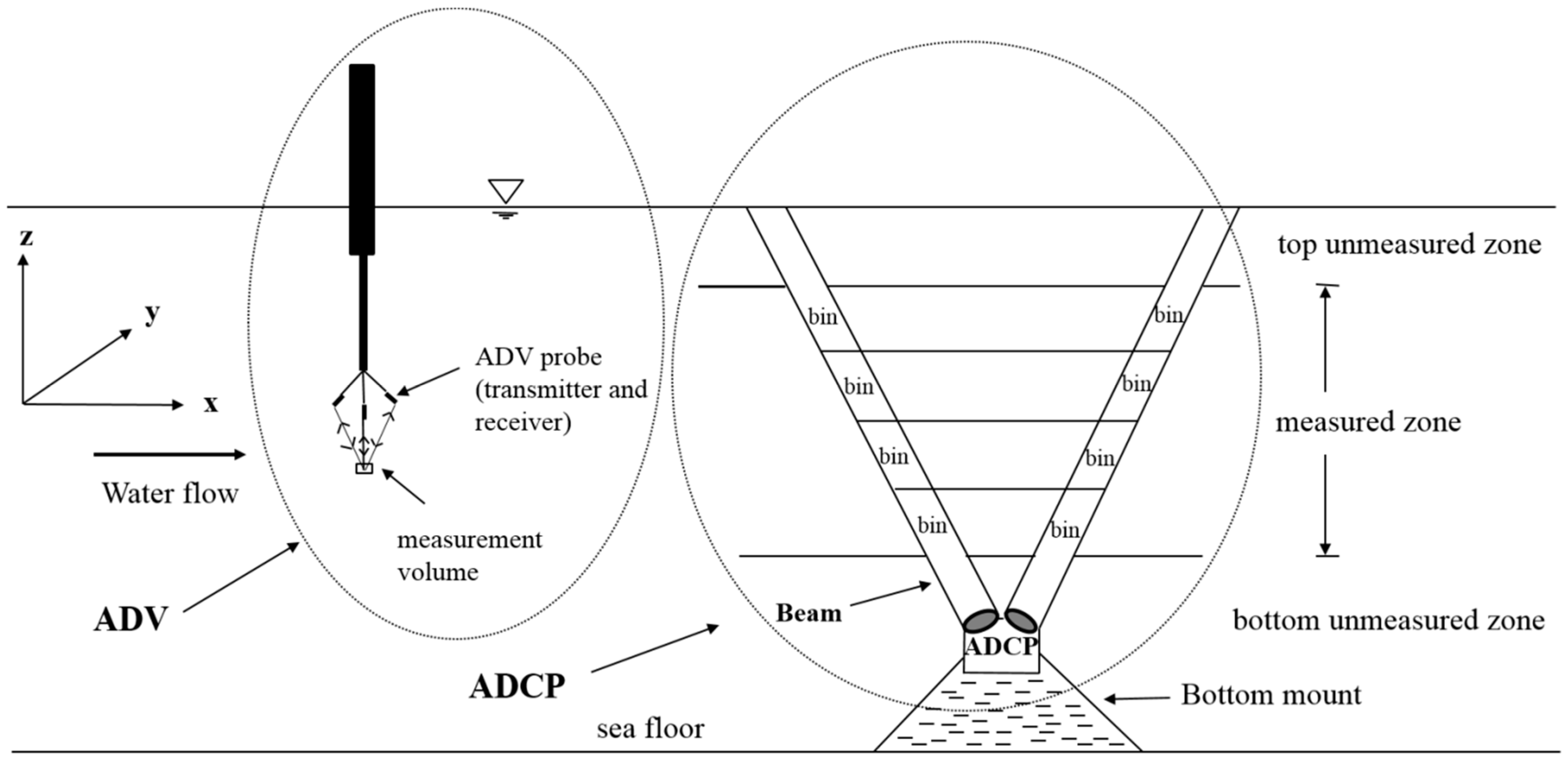
Figure 2.
Experimental setup in laboratory.

Figure 3.
Raw backscatter amplitude vs. concentration for two experiments with well-sorted (top panel) and mixed (lower panel) sand samples. Each case was repeated six times for each tested concentration (the central mark is median, the edges of each box are the 25th and 75th percentiles, and the whiskers show extremes).
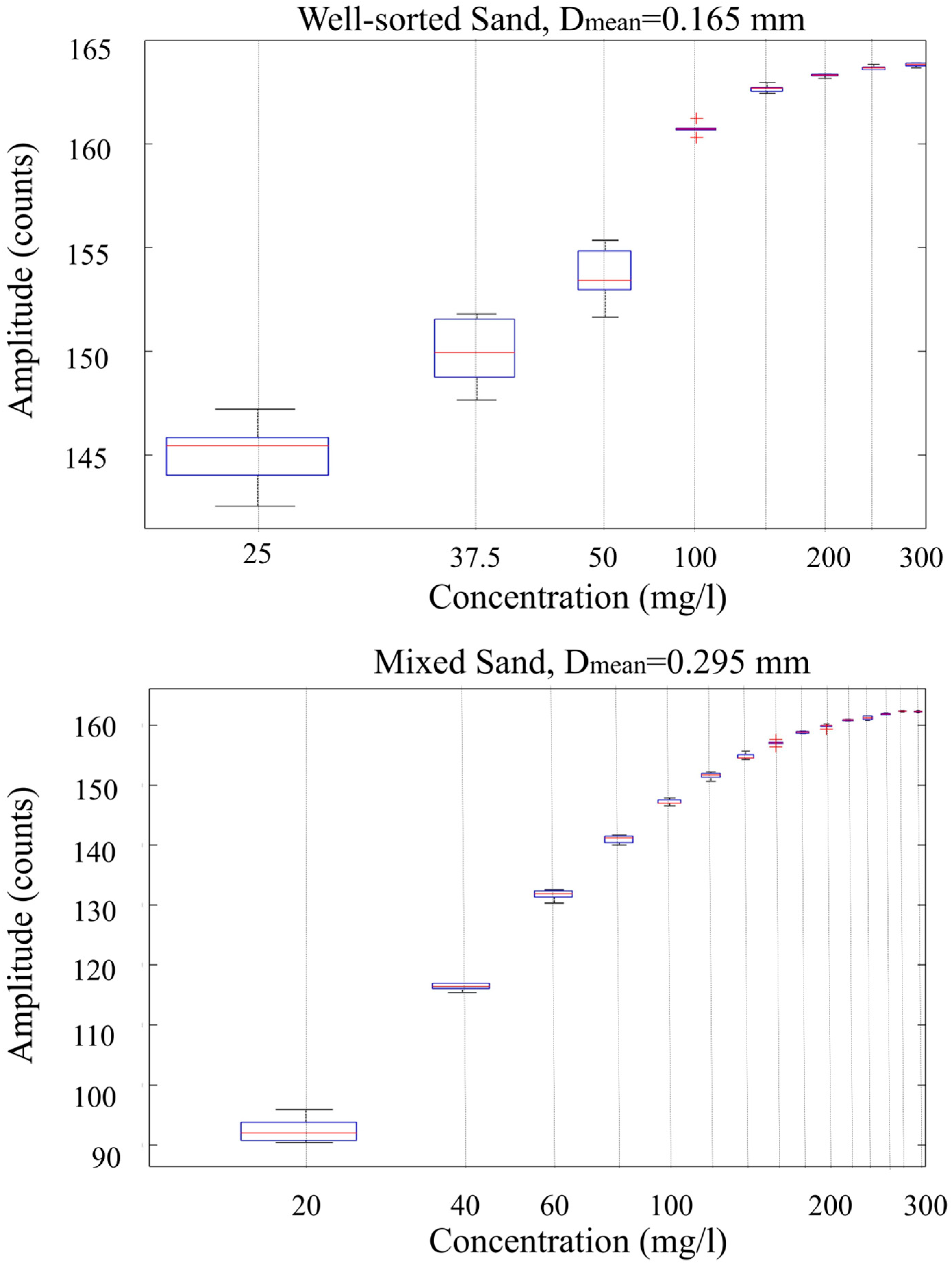
Figure 4.
Raw backscatter vs. concentration for five well-sorted sand cases. The boxes show median value and 95% confidence intervals, with each scenario represented by six trials.
Figure 4.
Raw backscatter vs. concentration for five well-sorted sand cases. The boxes show median value and 95% confidence intervals, with each scenario represented by six trials.

Figure 5.
Corrected mean backscattered amplitudes vs. suspended sediment concentration for each sieved fraction.
Figure 5.
Corrected mean backscattered amplitudes vs. suspended sediment concentration for each sieved fraction.

Figure 6.
Predicted vs. known concentrations for the well-sorted sand fractions, with predictions computed using Equations (10)–(12). RMSE = Root-mean-square error from the 1:1 line.
Figure 6.
Predicted vs. known concentrations for the well-sorted sand fractions, with predictions computed using Equations (10)–(12). RMSE = Root-mean-square error from the 1:1 line.
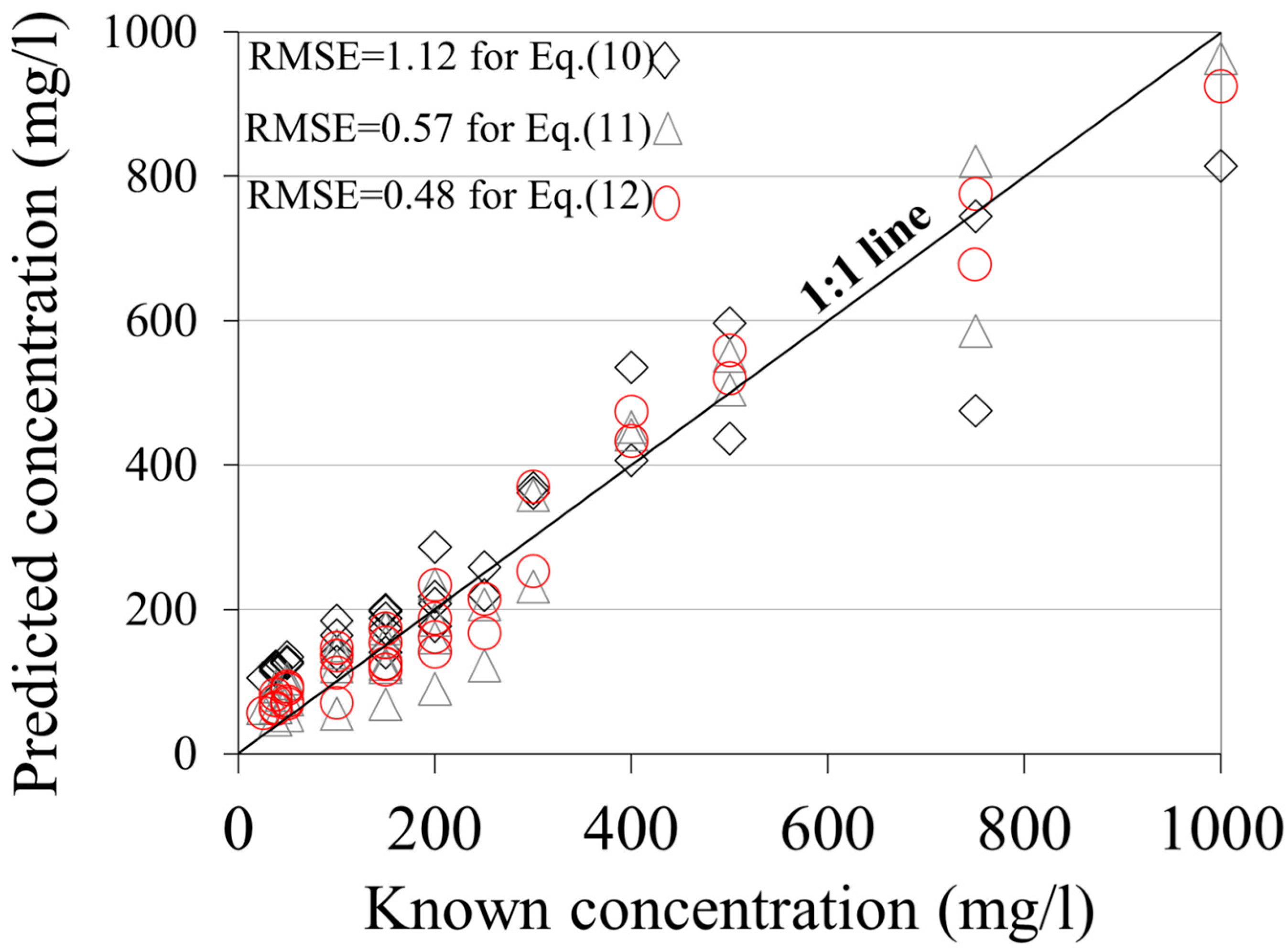
Figure 7.
Predicted vs. known concentrations for mixed-sand cases, based on Equations (13)–(15). RMSE = Root-mean-square error from the 1:1 line.
Figure 7.
Predicted vs. known concentrations for mixed-sand cases, based on Equations (13)–(15). RMSE = Root-mean-square error from the 1:1 line.

Figure 8.
Predicted vs. known concentrations for the well-sorted beach sand fractions from Folly Island, South Carolina, with predictions computed using Equations (19) and (20).
Figure 8.
Predicted vs. known concentrations for the well-sorted beach sand fractions from Folly Island, South Carolina, with predictions computed using Equations (19) and (20).


Table 1.
Summary of sand sizes and concentrations for which acoustic backscatter data were collected (+ and - signs indicate the availability and unavailability of the data, respectively) for experiments with well-sorted sands. Construction sand was sieved to yield the various size fractions.
Table 1.
Summary of sand sizes and concentrations for which acoustic backscatter data were collected (+ and - signs indicate the availability and unavailability of the data, respectively) for experiments with well-sorted sands. Construction sand was sieved to yield the various size fractions.
| Suspended Sediment Concentration (mg/L) | |||||||||||||||
|---|---|---|---|---|---|---|---|---|---|---|---|---|---|---|---|
| Dmean (mm) | 25 | 37.5 | 50 | 100 | 150 | 200 | 250 | 300 | 400 | 500 | 750 | 1000 | 1500 | 2000 | 3000 |
| 0.420 | + | + | + | + | + | + | + | + | + | + | + | + | + | + | + |
| 0.325 | + | + | + | + | + | + | + | + | + | + | + | + | + | + | - |
| 0.215 | + | + | + | + | + | + | + | + | + | + | + | + | + | - | - |
| 0.165 | + | + | + | + | + | + | + | + | - | + | - | - | - | - | - |
| 0.112 | + | + | + | + | + | - | - | - | - | - | - | - | - | - | - |
Table 2.
Summary of experiments with mixed sands created by adding together well-sorted construction sand fractions.
Table 2.
Summary of experiments with mixed sands created by adding together well-sorted construction sand fractions.
| Sample Name | Percentage of Each Sieve Fraction (% Mass) | Cg (D90/D10) | Dmean (mm) | Sieve Numbers of Fractions Used |
|---|---|---|---|---|
| Mix I | 20 | 5.19 | 0.258 | 40, 60, 80, 100, 200 |
| Mix II | 25 | 3.2 | 0.295 | 40, 60, 80, 100 |
| Mix III | 25 | 6.29 | 0.281 | 40, 60, 80, 200 |
| Mix IV | 25 | 6.13 | 0.239 | 40, 80, 100, 200 |
| Mix V | 25 | 2.8 | 0.208 | 60, 80, 100, 200 |
Table 3.
Sizes and concentrations tested using natural beach sand from Folly Beach, South Carolina, sieved to yield well-sorted fractions. Experimental apparatus was the same as with the construction sand.
Table 3.
Sizes and concentrations tested using natural beach sand from Folly Beach, South Carolina, sieved to yield well-sorted fractions. Experimental apparatus was the same as with the construction sand.
| Dmean (mm) | Concentration Range (mg/L) |
|---|---|
| 0.325 | 100–750 |
| 0.215 | 50–300 |
| 0.165 | 25–200 |
| 0.112 | 25–150 |
© 2017 by the author. Licensee MDPI, Basel, Switzerland. This article is an open access article distributed under the terms and conditions of the Creative Commons Attribution (CC BY) license (http://creativecommons.org/licenses/by/4.0/).
Share and Cite
MDPI and ACS Style
Öztürk, M. Sediment Size Effects in Acoustic Doppler Velocimeter-Derived Estimates of Suspended Sediment Concentration. Water 2017, 9, 529. https://doi.org/10.3390/w9070529
AMA Style
Öztürk M. Sediment Size Effects in Acoustic Doppler Velocimeter-Derived Estimates of Suspended Sediment Concentration. Water. 2017; 9(7):529. https://doi.org/10.3390/w9070529
Chicago/Turabian StyleÖztürk, Mehmet. 2017. "Sediment Size Effects in Acoustic Doppler Velocimeter-Derived Estimates of Suspended Sediment Concentration" Water 9, no. 7: 529. https://doi.org/10.3390/w9070529
Note that from the first issue of 2016, this journal uses article numbers instead of page numbers. See further details here.