Evaluating the Potentiality of Sentinel-2 for Change Detection Analysis Associated to LULUCF in Wallonia, Belgium


Scientific Institute of Public Service (ISSeP), rue du Chéra 200, 4000 Liege, Belgium
*
Author to whom correspondence should be addressed.
Land 2021, 10(1), 55; https://doi.org/10.3390/land10010055
Submission received: 14 December 2020
/
Revised: 5 January 2021
/
Accepted: 7 January 2021
/
Published: 9 January 2021
(This article belongs to the Special Issue Monitoring Land Cover Change: Towards Sustainability)
Abstract
:Land Use/Cover changes are crucial for the use of sustainable resources and the delivery of ecosystem services. They play an important contribution in the climate change mitigation due to their ability to emit and remove greenhouse gas from the atmosphere. These emissions/removals are subject to an inventory which must be reported annually under the United Nations Framework Convention on Climate Change. This study investigates the use of Sentinel-2 data for analysing lands conversion associated to Land Use, Land Use Change and Forestry sector in the Wallonia region (southern Belgium). This region is characterized by one of the lowest conversion rates across European countries, which constitutes a particular challenge in identifying land changes. The proposed research tests the most commonly used change detection techniques on a bi-temporal and multi-temporal set of mosaics of Sentinel-2 data from the years 2016 and 2018. Our results reveal that land conversion is a very rare phenomenon in Wallonia. All the change detection techniques tested have been found to substantially overestimate the changes. In spite of this moderate results our study has demonstrated the potential of Sentinel-2 regarding land conversion. However, in this specific context of very low magnitude of land conversion in Wallonia, change detection techniques appear to be not sufficient to exceed the signal to noise ratio.
1. Introduction
Land Use/Cover changes (LULCC) lie on a scale of severity that ranges from no alteration through modifications of varying intensity to a full transformation. The rate of change and the nature of the transitions differ in time and space. Some regions are relatively stable (e.g., permanent forest); whereas others areas are subject to rapid and persistent transformation (e.g., urban expansion of previously agricultural land). The increase of human population and technological development has been found to accelerate LULCC [1,2,3]. There is extensive literature on sudden land cover conversion resulting from manmade or natural phenomenon such as forest deterioration, agricultural magnification, natural disaster or urban sprawl. However, few studies focus on subtle land changes. The study of LULCC relies on both subtle and abrupt transitions and an improved understanding of the complex dynamic processes underlying the former would allow for more reliable projections and more realistic scenarios of future changes [4].
According to European statistics [5] only 1.6% of land cover type has changed during the 2006–2012 period. This number covers 39 countries which span over 5.86 million of km2. Among European countries, Belgium has one of the lowest mean annual land cover rates. Each year, only 0.1% of the total area (~30 km2) is converted to different land cover classes [6]. As such it is not surprising that many studies focus on African and Asian countries which have undergone major LULCC transformations. Africa has the largest annual rate of forest loss and reports from African countries documented that about 0.82 million km2 of forest have been converted into other land uses between 1990 and 2015 [7]. Asia has also experienced major LULCC conversions. As an example, Beijing’s urban area extent has quadrupled from 2000 and 2009 [8].
Annual LULCC information is valuable to aid in the formulation of socio-economic policies (e.g., European Common Agriculture) and data provision for environmental applications [3]. The impact of LULCC on the global climate via the carbon cycle has been highlighted from the early 1980s. It has been shown that terrestrial ecosystems act both as source and sink of carbon [4,9,10]. The anthropogenic emissions and removal associated to the sector of Land Use Land Use Change and Forestry (LULUCF) has to be inventoried annually under Article 4 of the United Nations Framework Convention on Climate Change (UNFCCC). This inventory is composed of land areas and changes in land area related with LULUCF activities. In practice, countries use a variety of sources of data for representing land use including agricultural census data, forest inventories, censuses for urban and natural land, land registry data and remote sensing data [11,12]. Remote sensing data has the advantage of generating a spatially explicit representation of land areas and their conversions. However, despite the advent of numerous remote sensing based monitoring systems expected to play a crucial role in Earth observation, the LULUCF inventory still relies mostly on census data and forest inventories.
In Europe, the Copernicus Land Monitoring Service (CLMS) jointly implemented by the European Environment Agency (EEA) and the European Commission DG Joint Research Centre (JRC), is providing different Earth observation products in the field of environmental terrestrial application. The oldest, CORINE Land Cover (CLC), was initiated in 1985 and proposes inventory of land cover [13]. These datasets cover the entire continent consistently, but with rather limited spatial detail (scale 1:100,000, Minimum Mapping Units 25 ha). This insufficient spatial detail limits the application of CLC for a precise LULCC [14]. Indeed, this data source has a poor reliability in surveying urban area (especially urban dispersion) since the minimum mapping unit is higher than most of the discontinuous patches. In particular, this is true for Belgium which is one of the most urbanized countries in Europe.
To complement CLC data, the CLMS has designed products called High Resolution Layer (HLR) which provide information on specific land cover characteristics (Imperviousness, Forests, Grassland, Water and Wetness, and Small Woody Feature) [15,16,17,18,19]. These datasets are based on satellite imagery through a combination of different sensors (optical and radar data). The reference year is 2015 and the spatial resolution is 20 m, except for the Small Woody Feature and Forest products which are based on data of a better resolution of 10 m.
Recently, the EEA and the European Commission have determined to develop a new generation of CLC products called CLC+. The CLC+ products suite consists of: CLC + Backbone, CLC + Core and CLC + Instances. CLC + Instances products should include a tailored product dedicated for LULUCF reporting called “CLC + LULUCF”. This component would have a temporal frequency of 1–3 years and a minimum cartographic unit of 0.005 km2. This upcoming CLC + LULUCF is designed to overcome the lack of CLC and HLR products to provide support for carrying out LULUCF inventories [20].
In addition to the previous products, the launch of ESA’s Sentinel-2 satellites in 2015 and 2017 with their high spatial and temporal resolution offers new opportunities for understanding how the Earth is changing. Sentinel 2A and B are characterized by a sun-synchronous orbit, phased at 180 to each other, and a frequent revisit cycle of 5 days [21]. The multi-temporal resolution ensures a better monitoring of LUC with the prospect of obtaining cloudless mosaics; whereas the wide spectral resolution facilitates the thematic identification of land cover [22] and the high spatial resolution allows for the identification of small objects, such as individual houses or landscapes structures [23,24].
This study investigates the potential of Sentinel-2 data for detecting lands conversions associated to the LULUCF sector in southern Belgium. The research tests the most widely used change detection techniques as described by [25] on a set of cloud- and snowless mosaics of Sentinel-2 from the years 2016 and 2018. The post-classification comparison logic will be tested in the case of the much debated use of per-pixel or per-object techniques to obtain a detailed from-to change information. The validation of this research use harmonized and comparable statistics on land use and land cover across the whole of the EU’s territory (Land Parcel Identification System (LPIS), Land Use/Cover Area frame Survey (LUCAS), CORINE Land Cover). This paper is an attempt to fill the gap related to subtle LULCC detection analysis and provides clues for using Copernicus Land Monitoring Services to support the LULUCF regulation. It also highlights the strengths and weaknesses of the most common change detection techniques. Finally, it discusses the use of Sentinel-2 data for measuring changes in carbon stocks resulting from direct human-induced land use.
The paper is organized into four sections. Section 2 gives a brief account of the change detection techniques and the reference data used in the research. Section 3 presents the results of the different techniques. Section 4 discusses the accuracy of the change maps and some challenges related to the use of Sentinel-2 data for LULUCF change detection. Finally, our conclusions are presented in Section 4.
2. Materials and Methods
2.1. Sentinel-2 Data Processing and Analysis
This study was undertaken in Wallonia, the southern part of Belgium (Figure 1). The region covers an area of 16,901 km2 with a population over 3.6 million. Two sets of Sentinel-2 images from 2016 and 2018 have been pre-processed according to the procedure adopted by [26]. Six cloudless and snowless mosaics composed of eight tiles of Sentinel-2 data have been produced. They cover three seasons: winter, spring and summer from both years. The weather conditions during the autumn period of both years did not permit to generate autumn mosaics due to an extended period of cloud cover.
The processing flow of the change detection analysis is shown in Figure 2. It involves the pre-processing of Sentinel-2 and the production of six mosaics of Sentinel-2 images. Then, the application of the most commonly used methods in change detection: (a) algebraic and, (b) post-classification [27]. The algebraic methods refer to bi-temporal approach which exploits only the summer mosaic of both years. In opposite, the post-classification methods involve the use of the six mosaics for a multi-temporal approach. The bi-temporal analysis was carried out using the ArcGIS Pro software and its raster calculator tool. A detailed process description of the pixel-based classification can be found in [26]. The object-based classification was also implemented in ArcGIS Pro software (Esri Inc. ArcGIS Pro (version 2.3.3). Software. Redlands, CA, USA: Esri Inc., 2018.).
2.1.1. Algebraic Change Detection
The algebraic change detection method involves the transformation of two original images into a new single-band image in which the areas of land cover change are highlighted [28]. The method is based on image algebra [27]. The most popularly techniques include: image differencing, image ratioing, index differencing and principal component analysis (PCA). Threshold selection for finding the change areas is a common procedure in algebra based change detection [29]. These techniques generates only binary change (i.e., change vs. no-change) [27]. They have the advantage of being based on the detection of physical changes between image dates. This avoids the errors introduced in post-classification where inaccuracies in the land cover classification between dates are propagated into the land cover change analysis [28].
Below are the different equations that have been applied on Sentinel-2 mosaics bands to generate the change maps using Raster Calculator tool (ArcGIS Pro):
- Image differencing [25]
- Image ratioing [25]:
- Spectral index differencing [25]:
In this research, we use four widely used spectral indices to extract land feature: (1) Normalized Vegetation Index (NDVI [30,31]), (2) Normalized Difference Built-up Index (NDBI [32]), (3) Brightness Index (BI [33]) and, (4) the second Brightness Index (BI2 [33])). We use only soil and vegetation indices due to their ability to characterize the most relevant land categories (forest land, cropland, grassland and settlement). We did not use water index because we assumed that this land category did not change much over the time. Image differencing was then applied to all spectral indices.
- Principal component analysis (PCA) [25]:
PCA is used to capture the maximum variance in a finite number of orthogonal components based on an eigenvector analysis of the data correlation matrix. It has been used in change detection for many years because of its capacity of enhancing the information on change. The basic premise of PCA is to reduce the dimensionality of a dataset consisting of a large number of interrelated variables, while retaining as much as possible the variation present in the dataset. This is achieved by transforming to a new set of variables, the principal components (PCs), which are uncorrelated, and which are ordered so that the first few retain most of the variation present in all of the original variables [28].
In this study, PCA has been used in two steps. First, it has determined which bands of the 10 bands Sentinel-2 data retain most of the variation (Table 1). The first four bands (B2, B3, B4, B5) account for 98.78% of the covariance with a percentage of eigen values higher than 1%. For these reasons, we only used B2, B3, B4 and, B5 to carry out the pre-classification analysis.
Second, the resulting PCs from 2018 have been compared with PCA images from 2016 through image differencing in order to generate change maps. Principal Components Analysis was performed using ArcGIS Pro.
2.1.2. Post-Classification Change Detection
The post-classification method is the comparative analysis of two independently produced classifications from different dates [25]. The post-classification comparison can be done in a pixel- or object-based manner. In the pixel based approach, the classification is performed at the raster cell level whereas the object-based approach groups pixels into homogenous units based on local variance criteria objects are created using local homogeneity criteria, merging spatially contiguous pixels [34,35,36]. It is generally argued that the object-based classification is more suitable for Very High Resolution (VHR) images where the pixel-based approach faces the challenge posed by higher spectral variation and mixed pixels [27,35]. Contrary to the image algebra method, these techniques provide from-to change information. They have the advantage to bypass the difficulties in change detection associated with the analysis of images acquired at different times of the year [37,38,39]. However, as mentioned before, they are highly sensitive to the individual classification accuracies [28] and the comparison of the classifications inevitability leads to overstating the extent of changes [40].
In this research, the pixel-based classification was performed according to the work of [26]. The object-based classification was conducted using ArcGIS Pro software. The segmentation was carried out using Segment Mean Shift of the Spatial Analyst toolbox and the classifier was Maximum Likelihood Classification. Training and validation datasets were the same as the work of [26]. The comparison of each independent classification was executed using Raster Calculator tool.
2.2. Reference Data
2.2.1. Land Parcel Identification System (LPIS)
In Wallonia, the land parcel identification system (LPIS) is called anonymous agricultural plot (AAP). The LPIS indicates the use of land in agricultural areas managed within the framework of the Common Agricultural Policy. The AAP is publicly available through the geoservices of Wallonia (https://geoservices.wallonie.be/arcgis/rest/services/AGRICULTURE/SIGEC_PARC_AGRI_ANON__2018/MapServer). This dataset gives the delineations of boundaries of agricultural fields, as well as the other relevant information assigned by farmers for each claim year. For this study, the AAP has been converted through a conversion table (Appendix D) to have only the distribution of grassland and cropland and thereby corresponds to the definitions of the categories of land as defined by reference [12].
2.2.2. CORINE Land Cover (CLC)
CORINE Land Cover is a land cover database that has been produced for 1990, 2000, 2006, 2012 and 2018 [41]. This inventory consists of 44 land cover classes and uses a minimum mapping unit of 0.25 km2. This classes are grouped into 5 land cover classes in the land cover change and statistics 2000–2018 (available at https://www.eea.europa.eu/data-and-maps/dashboards/land-cover-and-change-statistics. It is an interactive viewer that displays land cover statistics per country (Table 2).
2.2.3. Reference Points
The Land Use/Cover Area frame Survey (LUCAS) and the Water and Wetness (WAW) layer of the Copernicus land monitoring HLR have been used to produce the reference points of this study. The LUCAS database is a survey conducted by Eurostat which provides harmonized statistics on LUC across European Union. LUCAS is based on statistical calculations that interpret observations in the field. It is based on a standardized survey methodology in terms of a sampling plan, classifications, data collection processes and statistical estimators that are used to obtain harmonized and unbiased estimates of land use and land cover [42]. The database was converted into the 5 categories of land (forest land, cropland, grassland, wetland and settlement) as defined by Reference [12] through a conversion table (Appendix C). Both definitions of land categories were difficult to align perfectly because the classes nomenclature were not the same and the LULUCF land categories are really rigorous (e.g., a forest has to be of at least of 0.5 ha, 20% of trees and a height of 5 m). In addition, LUCAS nomenclature has been made to be harmonized and comparable at the EU scale and is not specific to the particularities of Belgium landscape. To take into account these limitations, all the points were further validated by means of the interpretation of the Sentinel-2 mosaics and aerial orthophotography available at (https://geoportail.wallonie.be/catalogue/647e383d-c74b-4ee6-bf48-a5ebc746e8 bf.html) from years 2016 and 2018. The Water and Wetness (WAW) layer of 2015 was used to address the lack of points in the “wetland” category of the LUCAS database. Points have been randomly allocated in the classes’ permanent water and permanent wet area. This stratified random sampling design enables to satisfy the accuracy assessment [43,44]. The resulting reference points are depicted in Figure 3 and the statistics are available in Table 3. In total, eight points have changed between 2016 and 2018. This gives a percentage of change of 0.37%. The area of land converted ranges from 0.02 to 0.33 km2.
3. Results
3.1. Algebraic Change Detection Results
The algebraic change detection analysis applied algebraic operations (differencing and ratioing) on the mosaic of summer 2018 and 2016. These mosaics have been chosen because they were acquired in the best period of the year for executing the image analysis (homogeneous vegetation status, good atmospheric conditions, good illumination and viewing angle). The selection of the bands of interest has been made through a principal component analysis (PCA) (Section 2.1.1).
Figure 4 is an illustration representing an example of land use change in Wallonia. The location of the observed changes is delimited by black polygons. In this area of interest, two polygons of forest land (A and B) in 2016 have been converted into settlement and one polygon of grassland in 2016 (C) has been converted into settlement in 2018. Figure 5 shows the results of the algebraic method and Table 4 presents the Walloon’ statistics of change associated to each algebra technique.
3.2. Post-Classification Results
Figure 6 shows the object-based post-classification results and Figure 7 the pixel-based post-classification results of the same area of interest (Figure 4). Table 5 and Table 6 presents the statistics of both post-classification techniques. The pixel-based classification has a higher overall accuracy (91.90% for 2016 and 91.70% for 2018) than the object-based classification (84.65% for 2016 and 76.56% for 2018). The percentage of unchanged pixels is close to the multiplication of the accuracies of each independent classifications (accuracies pixel-based = 0.84; unchanged pixels = 0.83/accuracies object-based = 0.64; unchanged pixels = 0.67). Table 7 reports the errors matrix in terms of estimated area proportion for the pixel-based classification.
3.3. Comparison with Validation Datasets
The change maps have been compared with three different datasets: (1) CORINE Land Cover, (2) Anonymous Agricultural Plot and (3) the reference points. Table 8 consists of a summary of the different results of the three validation datasets.
3.4. Accuracy Assessment
Appendix A and Appendix B present the confusion matrices of each change map using the 2141 reference points based on LUCAS and WAW database for the year 2016 and 2018. In addition, the overall accuracy (OA) was generated from the confusion matrix [36]. Figure 8, Figure 9 and Figure 10 show a graphical representation of the results for the OA, errors of omission (changed erroneously) and errors of commission (not changed erroneously). We also evaluated the statistical significance of the difference between the pixel-based classification and the object-based classification using the chi-square distribution with one degree of freedom. The test equation may be expressed as [45]:
The resulting matrix is presented in Table 9. The Chi squared test shows a relationship between both classifications. This is not surprising since both classifications were trained with the same training sample and the same classifier (Maximum Likelihood).
4. Discussion
As mentioned by reference [25], the selection of a suitable method of change detection for a given research is not straightforward. It depends on the remote sensing data, the study area and the type and magnitude of change. Four observations may be drawn from the results of this research.
First, the three validation datasets have highlighted the fact that the rate of LUC change in Belgium is very low. According to reference [6], Belgium is a country with one of the lowest mean annual land cover change rates in Europe. Each year, only 0.1% (~30 km2) of the total area is converted to different land cover classes whereas the European mean rate is 1.6%. The reference points give a land conversion rate of 0.4% in Wallonia (~70 km2)) and enable the identification of the most converted land areas in Wallonia. They are grassland (−0.41%) and settlement (+1.21%) (Table 3). This is not surprising since grassland is the main source for artificial land take in the country. The AAP also identifies grassland as a category of land which undergoes a notable conversion (2.55%). However, this dataset does not provide the direction of changes. Meanwhile, the agricultural area of CLC shows a change of −0.13% (Table 2 and Table 7). Unlike the other validation datasets, it points out a major wetland conversion which is in fact the result of the minimum mapping unit of CLC (0.25 km2) which is not sufficient to properly map most of wetland areas in Belgium.
Second, when comparing the algebraic and post-classification methods, the algebraic methods provide a percentage of change closer to the reality of LULUCF changes (Table 8 and Table 9). The change maps of the algebraic methods show a change percentage ranging from 1.6% (ratio B4) to 15.76% (PC3) and an overall accuracy (OA) ranging from 82.6% (BI2 differencing) to 98.1% (ratio B4). According to the classification standard of [46], most of these overall accuracies are considered as satisfactory because they are higher than 85%. Although, the algebraic methods overall accuracies are high, these numbers are mainly driven by the large proportion of unchanged points. The results of the post-classification methods differ further from the real change percentage (from 16.6% to 32.8%) and have lower overall accuracies (Table 5 and Table 6). As mentioned by reference [47] determining land changes by overlaying maps that have the same categories from two points in time makes sense when the map are perfectly accurate. In this study, the maps are not perfectly accurate (OApixel-based = 91.9% and 91.7%; OAobject-based = 84.7% and 76.6%) and the amount of error is too large to ignore. Moreover, according to the reference points, the amount of change is 0.4%, while the errors in maps is significantly higher (Errorpixel-based = 8.1% and 8.3%; Errorobject-based = 15.3% and 23.4%. Hence, errors in each individual map result in differences between the two maps.
Despite having more misclassification and misregistration errors, Figure 10 shows that the post-classification methods are the most sensitive change detection technique. Among them, the object-based technique gives the most satisfying results when looking at identifying the location of observed changes (6 reference point of “change” have been correctly attributed to “change” in the change map). However, we did not observe a reduction of the small spurious change within the extent of each object that should results in a high spectral variability in the pixel-based classification [35]. Furthermore, the object-based technique has also the most important commission errors (652 reference points of “no change” have been erroneously attributed to “change” in the change map). In conclusion, all of the change detection techniques substantially overestimated the changes.
Third, the use of Sentinel-2 data for LULCC detection can be summarized by the following points. In terms of spatial scale, the 10 m spatial resolution is sufficient to delineate individual geographic objects of interest. The visualization of change maps has shown that the converted land areas in Wallonia range from 20 pixels to 3300 pixels. Regarding the temporal scale, Sentinel-2A is available since June 2015 and should have a lifespan of 7 years. A second generation should follow for 7 additional years. Sentinel-2A and 2B have a high revisit time of 5 days ensuring the production of several cloud-free mosaics per year that minimizes the seasonal phenological differences. Furthermore, the twin satellites are deployed in polar sun-synchronous orbit which ensures that the angle of sunlight upon the Earth’s surface is consistently maintained which limits the shadow effects. Consequently, Sentinel-2 provides high resolution images for the operational monitoring of land and the production of land-change detection maps.
Finally, the results of the change detection applied in the Walloon context of land conversion associated to the LULUCF sector shows its limits in precisely identifying the changes. On account of the low rate of land conversion in Wallonia (~0.4%; corresponding to ~70km2 of change), we reach a critical point where all techniques face difficulties to properly identify land conversion. As mentioned in the above point, Sentinel-2 data are not responsible for these moderate results. In addition, changing the temporal window from 2 years to 5 or more years would not improve significantly the results since the CLC data from 2006 to 2018 (Table 2) has not shown any increase of the magnitude of change. Similarly, the possibility of increasing the classification accuracy is very limited when reaching the 92% of overall accuracy. And if so, improving a few percent would still be too few to properly map the changes. As an example, two classifications of 98% of overall accuracy would make 96% of land correctly allocated in the change map and 4% of errors (~700 km2) for only 70 km2 of real changes.
In future, similar research should concentrate on (1) post-processing, (2) the combination of methods and (3) AI-based change detection. Nevertheless, it is essential to bear in mind that the post-processing could interfere with the automatic nature of the approach as well as its wide-scale implementation e.g., through the use of regional databases. Regarding the combination of methods, it is likely to propagate errors which would impede the final results. In recent years, integrated artificial intelligence technology has become a research focus in developing new change detection methods. Several studies have suggested that they could outperform the traditional change detection methods.
5. Conclusions
Gaining a better understanding of carbon cycle and climate change requires accurate information on land conversion. The recent launch of Sentinel-2 satellites provides new opportunities for studying LUC changes on a regional and global scale. A wide variety of studies have analyzed significant LUC changes such as massive forest deterioration or rapid urbanization in developing countries. Only a few have focused on more developed countries undergoing a low land conversion rate such as EU countries. In research explored the effectiveness of Sentinel-2 data to detect changes related to the LULUCF sector in Wallonia, Belgium. The approach tested the most commonly accepted change detection techniques in order to evaluate the capability of Sentinel-2 data to account for low land conversion. Our results suggest that the rate of conversion is too low to precisely identify changes. All the change detection techniques have been found to overestimate the change. We consider that Sentinel-2 data have a great potential for LUC change detection analysis. However, change detection capabilities are largely determined by whether the applied change magnitude exceeds the signal to noise ratio [48].
Author Contributions
O.C. is the main author of this manuscript. She processed the data and conducted the change detection analysis and the validation. S.P. made a substantial contribution in the processing of the Sentinel-2 data for the multi-temporal analysis and offered valuable comments on the methods and manuscript. B.B. conceived the original idea of the study. E.H. supervised the research. Please turn to the CRediT taxonomy for the term explanation. Authorship must be limited to those who have contributed substantially to the work reported. All authors have read and agreed to the published version of the manuscript.
Funding
This research was conducted in the framework of the “EO4LULUCF” project, which was funded by an internal fund of Institut Scientifique de Service Public Moerman (ISSeP).
Informed Consent Statement
Informed consent was obtained from all subjects involved in the study.
Acknowledgments
The authors would like to thank the European Union’s Earth Observation Programme Copernicus and Eurostat for the provision of the LUCAS database.
Conflicts of Interest
The authors declare no conflict of interest.
Appendix A

Table A1.
Confusion matrix of the algebraic methods. The PCA is the most sensitive technique of the pre-classification method with 3 locations of change correctly labelled within the change map of the PC1. The second-best technique is index differencing (NDVI, NDBI and BI) which have correctly labelled 1 location of change. The overall accuracy (OA) of each technique is expressed at the right side of the table.
| Reference Points | |||||
| change | no change | Total | |||
| B2 differencing | change | 0 | 8 | 8 | |
| no change | 172 | 1961 | 2133 | OA = 91.6% | |
| Total | 172 | 1969 | 2141 | ||
| Reference Points | |||||
| change | no change | Total | |||
| B3 differencing | change | 0 | 8 | 8 | |
| no change | 154 | 1979 | 2133 | OA = 92.4% | |
| Total | 154 | 1987 | 2141 | ||
| Reference Points | |||||
| change | no change | Total | |||
| B4 differencing | change | 0 | 8 | 8 | |
| no change | 128 | 2005 | 2133 | OA = 93.6% | |
| Total | 128 | 2013 | 2141 | ||
| Reference Points | |||||
| change | no change | Total | |||
| B5 differencing | change | 0 | 8 | 8 | |
| no change | 225 | 1908 | 2133 | OA = 89.1% | |
| Total | 225 | 1916 | 2141 | ||
| Reference Points | |||||
| change | no change | Total | |||
| Ratio B2 | change | 0 | 8 | 8 | |
| no change | 200 | 1933 | 2133 | OA = 90.3% | |
| Total | 200 | 1941 | 2141 | ||
| Reference Points | |||||
| change | no change | Total | |||
| Ratio B3 | change | 0 | 8 | 8 | |
| no change | 271 | 1862 | 2133 | OA = 87.0% | |
| Total | 271 | 1870 | 2141 | ||
| Reference Points | |||||
| change | no change | Total | |||
| Ratio B4 | change | 0 | 8 | 8 | |
| no change | 32 | 2101 | 2133 | OA = 98.1% | |
| Total | 32 | 2109 | 2141 | ||
| Reference Points | |||||
| change | no change | Total | |||
| Ratio B5 | change | 0 | 8 | 8 | |
| no change | 274 | 1859 | 2133 | OA = 86.8% | |
| Total | 274 | 1867 | 2141 | ||
| Reference Points | |||||
| change | no change | Total | |||
| PC1 | change | 3 | 5 | 8 | |
| no change | 192 | 1941 | 2133 | OA = 90.8% | |
| Total | 195 | 1946 | 2141 | ||
| Reference Points | |||||
| change | no change | ||||
| PC2 | change | 1 | 7 | 8 | |
| no change | 232 | 1901 | 2133 | OA = 88.8% | |
| Total | 233 | 1908 | 2141 | ||
| Reference Points | |||||
| change | no change | ||||
| PC3 | change | 1 | 7 | 8 | |
| no change | 309 | 1824 | 2133 | OA = 85.2% | |
| Total | 310 | 1831 | 2141 | ||
| Reference Points | |||||
| NDVI differencing | change | no change | |||
| change | 1 | 7 | 8 | ||
| no change | 173 | 1960 | 2133 | OA = 91.6% | |
| Total | 174 | 1967 | 2141 | ||
| Reference Points | |||||
| NDBI differencing | change | no change | Total | ||
| change | 1 | 7 | 8 | ||
| no change | 200 | 1933 | 2133 | OA = 90.3% | |
| Total | 201 | 1940 | 2141 | ||
| Reference Points | |||||
| BI differencing | change | no change | Total | ||
| change | 0 | 8 | 8 | ||
| no change | 95 | 2038 | 2133 | OA = 95.2% | |
| Total | 95 | 2046 | 2141 | ||
| Reference Points | |||||
| BI2 differencing | change | no change | Total | ||
| change | 1 | 7 | 8 | ||
| no change | 365 | 1768 | 2133 | OA = 82.6% | |
| Total | 366 | 1775 | 2141 | ||
Appendix B
Table A2.
Confusion matrix of the post-classification methods. The object-based is the most sensitive technique with 6 location of change correctly labelled whereas the pixel-based has only 1 location of change correctly attributed. The overall accuracy (OA) of each technique is expressed at the right side of the table.
| Reference Points | |||||
| change | no change | Total | |||
| Pixel-based | change | 1 | 7 | 8 | |
| no change | 342 | 1791 | 2133 | OA =83.7% | |
| Total | 343 | 1798 | 2141 | ||
| Reference Points | |||||
| change | no change | Total | |||
| Object-based | change | 6 | 2 | 8 | |
| no change | 652 | 1481 | 2133 | OA =69.5% | |
| Total | 658 | 1483 | 2141 | ||
Appendix C
Table A3.
Conversion table from LUCAS nomenclature to LULUCF categories of land.
| LUCAS | LULUCF Categories of Land | ||
|---|---|---|---|
| A00 Artificial land | A10 Roofed built-up areas | A11 | 5 |
| A12 | 5 | ||
| A13 | 5 | ||
| A20 Artificial non-built up areas | A21 | 5 | |
| A22 | 5 | ||
| A30 other Artificial areas | 5 | ||
| B00 Cropland | B10 Cereals | B11 | 2 |
| B12 | 2 | ||
| B13 | 2 | ||
| B14 | 2 | ||
| B15 | 2 | ||
| B16 | 2 | ||
| B17 | 2 | ||
| B18 | 2 | ||
| B19 | 2 | ||
| B20 Root Crops | B21 | 2 | |
| B22 | 2 | ||
| B23 | 2 | ||
| B30 Non-premanent industrial Crops | B31 | 2 | |
| B32 | 2 | ||
| B33 | 2 | ||
| B34 | 2 | ||
| B35 | 2 | ||
| B36 | 2 | ||
| B37 | 2 | ||
| B40 Dry pulse, vegetable and Flowers | B41 | 2 | |
| B42 | 2 | ||
| B43 | 2 | ||
| B44 | 2 | ||
| B45 | 2 | ||
| B50 Fodder Crops | B51 | 3 | |
| B52 | 3 | ||
| B53 | 3 | ||
| B54 | 3 | ||
| B55 | 3 | ||
| B70 Permanent crops | B71 | 2 | |
| B72 | 2 | ||
| B73 | 2 | ||
| B74 | 2 | ||
| B75 | 2 | ||
| B76 | 2 | ||
| B77 | 2 | ||
| B80 Other Permanent crops | B81 | 2 | |
| B82 | 2 | ||
| B83 | 2 | ||
| B84 | 2 | ||
| C00 Woodland | C10 Broad Leaved woodland | 1 | |
| C20 Coniferous woodland | C21 | 1 | |
| C22 | 1 | ||
| C23 | 1 | ||
| C30 Mixed woodland | C31 | 1 | |
| C32 | 1 | ||
| C33 | 1 | ||
| D00 Shrubland | D10 Shrubland with sparse tree cover | 1 | |
| D20 Shrubland without tree cover | 3 | ||
| E00 Grassland | E10 Grassland with sparese tree/shrub cover | 3 | |
| E20 Grassland without tree/shrub cover | 3 | ||
| E30 Spontaneously re-vegetaed surfaces | 3 | ||
| F00 Bare land and Lichens/Moss | F10 Rocks and stones | 5 | |
| F20 Sand | 5 | ||
| F30 Lichen and moss | NA | ||
| F40 other bare soil | 4 | ||
| G00 Water areas | G10 Inland water bodies | G11 | 4 |
| G12 | 4 | ||
| G20 Inland running water | G21 | 4 | |
| G22 | 4 | ||
| G30 Transitional water bodies | 4 | ||
| G50 Glaciers, permanent snow | NA | ||
| H00 Wetland | H10 inland wetlands | H11 | 3 |
| H12 | 3 | ||
| H20 Coastal wetland | H21 | NA | |
| H22 | NA | ||
| H23 | NA | ||
Appendix D
Table A4.
Conversion table from AAP nomenclature to LULUCF categories of land.
| AAP Nomenclature | Agricultural Classes | LULUCF Categories of Land |
|---|---|---|
| 6 | Prairie et fourrage | 3 |
| 36 | Epeautre | 2 |
| 37 | Sarrasin | 2 |
| 39 | Céréales ET légumineuses | 2 |
| 42 | Tournesol | 2 |
| 43 | Soja | 2 |
| 45 | Lin oléagineux | 2 |
| 46 | Autres oléagineux | 2 |
| 51 | Pois protéagineux | 2 |
| 53 | Lupin doux | 2 |
| 55 | Autres protéagineux | 2 |
| 71 | Betterave fourragère | 2 |
| 72 | Trèfles | 2 |
| 73 | Luzerne | 2 |
| 80 | Jachère | 3 |
| 81 | Couvert naturel/spontané | 3 |
| 85 | Autres couverts semés | 2 |
| 91 | Betterave sucrière | 2 |
| 96 | Cultures horticoles non-comestibles | 2 |
| 99 | Autres | 3 |
| 201 | Maïs ensilage | 2 |
| 202 | Maïs grain | 2 |
| 311 | Froment d’hiver | 2 |
| 312 | Froment de printemps | 2 |
| 321 | Orge d’hiver | 2 |
| 322 | Orge de printemps | 2 |
| 323 | Orge de brasserie | 2 |
| 331 | Seigle d’hiver | 2 |
| 332 | Seigle de printemps | 2 |
| 341 | Avoine d’hiver | 2 |
| 342 | Avoine de printemps | 2 |
| 351 | Triticale d’hiver | 2 |
| 352 | Triticale de printemps | 2 |
| 381 | Sorgho | 2 |
| 382 | Quinoa | 2 |
| 511 | Pois protéagineux d’hiver | 2 |
| 512 | Pois protéagineux de printemps | 2 |
| 521 | Fèves et Féveroles d’hiver | 2 |
| 522 | Fèves et Féveroles de printemps | 2 |
| 541 | Mélange protéagineux d’hiver + céréales ou autres espèces | 2 |
| 542 | Mélange protéagineux de printemps + céréales ou autres espèces | 2 |
| 743 | Autres fourrages | 3 |
| 851 | Couvert favorisant la faune | 2 |
| 872 | Chanvre non textile (culture soumise à autorisation préalable au semis) | 2 |
| 881 | Angélique | 2 |
| 884 | Miscanthus | 2 |
| 895 | Boisement de terre agricole (art 31 du R.(CE) 1257/1999)—dérogation | 2 |
| 901 | Pomme de terre (non hâtives) | 2 |
| 902 | Pomme de terre (plants) | 2 |
| 903 | Pomme de terre féculière | 2 |
| 904 | Pomme de terre (arrachage avant le 1er août) | 2 |
| 905 | Pomme de terre (primeur, arrachage avant le 20 juin) | 2 |
| 921 | Lin textile | 2 |
| 922 | Chanvre textile | 2 |
| 931 | Pois récoltés à l’état frais, pois de conserverie | 2 |
| 951 | Autres légumes | 2 |
| 952 | Cultures maraîchères sous verre | 2 |
| 953 | Plantes aromatiques | 2 |
| 957 | Plantes médicinales | 2 |
| 962 | Sapins de Noël | 2 |
| 966 | Légume légumineuse | 2 |
| 4111 | Colza d’hiver | 2 |
| 4112 | Navette d’hiver (graines) | 2 |
| 4121 | Colza de printemps | 2 |
| 7431 | Ortie | 2 |
| 7433 | Carotte | 2 |
| 9201 | Noisetier | 2 |
| 9410 | Haricots de conserverie | 2 |
| 9515 | Endives (chicons) | 2 |
| 9516 | Cultures fruitières annuelles—Fraises | 2 |
| 9520 | Pépinières de plants fruitiers ou de plantes ornementales | 2 |
| 9548 | Choux—Légumes | 2 |
| 9741 | Cultures fruitière pluriannuelles-basses tiges | 2 |
| 9811 | Chicorée à inuline | 2 |
| 9812 | Chicorée à café | 2 |
| 9821 | Tabac | 2 |
References
- Goldewijk, K.K. Estimating global land use change over the past 300 years: The HYDE Database. Glob. Biogeochem. Cycles 2001, 15, 417–433. [Google Scholar] [CrossRef]
- Ramankutty, N.; Foley, J.A. Estimating historical changes in global land cover: Croplands from 1700 to 1992. Glob. Biogeochem. Cycles 1999, 13, 997–1027. [Google Scholar] [CrossRef]
- Gómez, C.; White, J.; Wulder, M.A. Optical remotely sensed time series data for land cover classification: A review. ISPRS J. Photogramm. Remote. Sens. 2016, 116, 55–72. [Google Scholar] [CrossRef] [Green Version]
- Lambin, E.F.; Geist, H.J.; Lepers, E. DYNAMICS OFLAND-USE ANDLAND-COVERCHANGE INTROPICALREGIONS. Annu. Rev. Environ. Resour. 2003, 28, 205–241. [Google Scholar] [CrossRef] [Green Version]
- European Environment Agency. Landscapes in Transition. An Account of 25 Years of Land Cover Change in Europe. EEA Rep. 2017, 10, 226. [Google Scholar] [CrossRef]
- European Environment Agency. Belgium. 2017. Available online: https://www.eea.europa.eu/publications/air-quality-in-europe-2017 (accessed on 8 January 2021).
- Tian, H.; Lu, C.; Yang, J.; Banger, K.; Huntzinger, D.N.; Schwalm, C.R.; Michalak, A.M.; Cook, R.; Ciais, P.; Hayes, D.J.; et al. Global patterns and controls of soil organic carbon dynamics as simulated by multiple terrestrial biosphere models: Current status and future directions. Glob. Biogeochem. Cycles 2015, 29, 775–792. [Google Scholar] [CrossRef]
- Sorichetta, A.; Nghiem, S.V.; Masetti, M.; Linard, C.; Richter, A. Transformative Urban Changes of Beijing in the Decade of the 2000s. Remote. Sens. 2020, 12, 652. [Google Scholar] [CrossRef] [Green Version]
- Sagan, C.; Toon, O.B.; Pollack, J.B.; Mumma, M.J.; Buhl, D.; Chin, G.; Deming, D.; Espenak, F.; Kostiuk, T.; Zipoy, D. Anthropogenic Albedo Changes and the Earth’s Climate. Science 1979, 206, 1363–1368. [Google Scholar] [CrossRef]
- Houghton, R.A. Terrestrial sources and sinks of carbon inferred from terrestrial data. Tellus B Chem. Phys. Meteorol. 1996, 48, 420–432. [Google Scholar] [CrossRef] [Green Version]
- Representation, C.; Guidelines, I.; Greenhouse, N.; Inventories, G. Chapter 3 Consistent Representation of. 2006. Available online: https://www.ipcc-nggip.iges.or.jp/public/2006gl/pdf/4_Volume4/V4_03_Ch3_Representation.pdf (accessed on 8 January 2021).
- IPCC. Lignes Directrices 2006 Du GIEC Pour Les Inventaires Nationaux de Gaz à Effet de Serre.Volume 4: Agriculture, Foresterie et Autres Affectations des Terres: Chapitre 1 Introduction; IPCC: Saint-Aubin, France, 2006; pp. 1–25. [Google Scholar]
- Manakos, I.; Braun, M. Land Use and Land Cover Mapping in Europe; Springer: London, UK, 2014; Volume 18. [Google Scholar]
- Rosina, K.; Silva, F.B.; Vizcaino, P.; Herrera, M.M.; Freire, S.; Schiavina, M. Increasing the detail of European land use/cover data by combining heterogeneous data sets. Int. J. Digit. Earth 2018, 13, 602–626. [Google Scholar] [CrossRef]
- Langanke, T. Copernicus Land Monitoring Service—High Resolution Layer Imperviousness. 2016. Available online: https://land.copernicus.eu/pan-european/high-resolution-layers (accessed on 8 January 2021).
- European Environment Agency. High Resolution Layer Forest: Product Specifications; European Commission: Brussels, Belgium, 2017; p. 38.
- Langanke, T. Copernicus Land Monitoring Service—High Resolution Layer Grassland, Product Specifications; European Commission: Brussels, Belgium, 2016. [Google Scholar]
- European Environment Agency. Copernicus Land Monitoring Service—High Resolution Layer Water and Wetness; European Commission: Brussels, Belgium, 2018.
- European Environmental Agency. Copernicus Land Monitoring Service—High Resolution Layer Small Woody Features—2015 Reference Year; European Commission: Brussels, Belgium, 2015; pp. 1–30.
- Copernicus. Workshop Summary Using Copernicus Land Monitoring Service (CLMS) to Support the Land Use, Land Use Change and Forestry (LULUCF) Regulation; European Commission: Brussels, Belgium, 2019. [Google Scholar]
- Drusch, M.; Del Bello, U.; Carlier, S.; Colin, O.; Fernandez, V.M.; Gascon, F.; Hoersch, B.; Isola, C.; Laberinti, P.; Martimort, P.; et al. Sentinel-2: ESA’s Optical High-Resolution Mission for GMES Operational Services. Remote. Sens. Environ. 2012, 120, 25–36. [Google Scholar] [CrossRef]
- Immitzer, M.; Vuolo, F.; Atzberger, C. First Experience with Sentinel-2 Data for Crop and Tree Species Classifications in Central Europe. Remote. Sens. 2016, 8, 166. [Google Scholar] [CrossRef]
- Radoux, J.; Chomé, G.; Jacques, D.C.; Waldner, F.; Bellemans, N.; Matton, N.; Lamarche, C.; D’Andrimont, R.; Defourny, P. Sentinel-2’s Potential for Sub-Pixel Landscape Feature Detection. Remote. Sens. 2016, 8, 488. [Google Scholar] [CrossRef] [Green Version]
- Lefebvre, A.; Sannier, C.; Corpetti, T. Monitoring Urban Areas with Sentinel-2A Data: Application to the Update of the Copernicus High Resolution Layer Imperviousness Degree. Remote. Sens. 2016, 8, 606. [Google Scholar] [CrossRef] [Green Version]
- Lu, D.; Mausel, P.; Brondízio, E.; Moran, E. Change detection techniques. Int. J. Remote. Sens. 2004, 25, 2365–2401. [Google Scholar] [CrossRef]
- Close, O.; Beaumont, B.; Petit, S.; Fripiat, X.; Hallot, E. Use of Sentinel-2 and LUCAS Database for the Inventory of Land Use, Land Use Change, and Forestry in Wallonia, Belgium. Land 2018, 7, 154. [Google Scholar] [CrossRef] [Green Version]
- Hussain, M.; Chen, D.; Cheng, A.; Wei, H.; Stanley, D. Change detection from remotely sensed images: From pixel-based to object-based approaches. ISPRS J. Photogramm. Remote. Sens. 2013, 80, 91–106. [Google Scholar] [CrossRef]
- Deng, J.S.; Wang, K.; Deng, Y.H.; Qi, G.J. PCA-based land-use change detection and analysis using multitemporal and multisensor satellite data. Int. J. Remote. Sens. 2008, 29, 4823–4838. [Google Scholar] [CrossRef]
- Asokan, A.; Anitha, J. Change detection techniques for remote sensing applications: A survey. Earth Sci. Inform. 2019, 12, 143–160. [Google Scholar] [CrossRef]
- Tucker, C.J. Red and Photographic Infrared Linear Combinations for Monitoring Vegetation. Remote Sens. Environ. 1979, 8, 127. [Google Scholar] [CrossRef] [Green Version]
- Ji, L.; Peters, A.J. Assessing vegetation response to drought in the northern Great Plains using vegetation and drought indices. Remote. Sens. Environ. 2003, 87, 85–98. [Google Scholar] [CrossRef]
- Zha, Y.; Gao, J.; Ni, S. Use of normalized difference built-up index in automatically mapping urban areas from TM imagery. Int. J. Remote. Sens. 2003, 24, 583–594. [Google Scholar] [CrossRef]
- Escadafal, R. Remote sensing of arid soil surface color with Landsat thematic mapper. Adv. Space Res. 1989, 9, 159–163. [Google Scholar] [CrossRef]
- Cheţan, M.A.; Dornik, A.; Urdea, P. Comparison of Object and Pixel-Based Land Cover Classification through Three Su-pervised Methods. J. Geodasy Geoinf. Land Manag. 2017. [Google Scholar] [CrossRef]
- Chen, G.; Hay, G.J.; Carvalho, L.M.T.; Wulder, M.A. Object-based change detection. Int. J. Remote. Sens. 2012, 33, 4434–4457. [Google Scholar] [CrossRef]
- Pierce, J.K.B. Accuracy Optimization for High Resolution Object-Based Change Detection: An Example Mapping Regional Urbanization with 1-m Aerial Imagery. Remote. Sens. 2015, 7, 12654–12679. [Google Scholar] [CrossRef] [Green Version]
- Coppin, P.; Jonckheere, I.; Nackaerts, K.; Muys, B.; Lambin, E. Review ArticleDigital change detection methods in ecosystem monitoring: A review. Int. J. Remote. Sens. 2004, 25, 1565–1596. [Google Scholar] [CrossRef]
- Tewkesbury, A.P.; Comber, A.J.; Tate, N.J.; Lamb, A.; Fisher, P.F. A critical synthesis of remotely sensed optical image change detection techniques. Remote. Sens. Environ. 2015, 160, 1–14. [Google Scholar] [CrossRef] [Green Version]
- Wu, C.; Du, B.; Cui, X.; Zhang, L. A post-classification change detection method based on iterative slow feature analysis and Bayesian soft fusion. Remote. Sens. Environ. 2017, 199, 241–255. [Google Scholar] [CrossRef]
- Huang, L.; Fang, Y.; Zuo, X.; Yu, X. Automatic Change Detection Method of Multitemporal Remote Sensing Images Based on 2D-Otsu Algorithm Improved by Firefly Algorithm. J. Sens. 2015, 2015, 1–8. [Google Scholar] [CrossRef] [Green Version]
- Büttner, G.; Kostztra, B.; Soukup, T.; Sousa, A.; Langanke, T. CLC2018 Technical Guidelines. 2017. Available online: https://land.copernicus.eu/user-corner/technical-library/clc2018technicalguidelines_final.pdf (accessed on 8 January 2021).
- EUROSTAT. LUCAS 2015 (Land Use/Cover Area Frame Survey), Quality Report; European Commission: Brussels, Belgium, 2015.
- Olofsson, P.; Foody, G.M.; Herold, M.; Stehman, S.V.; Woodcock, C.E.; Wulder, M.A. Good practices for estimating area and assessing accuracy of land change. Remote. Sens. Environ. 2014, 148, 42–57. [Google Scholar] [CrossRef]
- Stehman, S.V.; Foody, G.M. Key issues in rigorous accuracy assessment of land cover products. Remote. Sens. Environ. 2019, 231, 111199. [Google Scholar] [CrossRef]
- Foody, G.M. Thematic Map Comparison. Photogramm. Eng. Remote. Sens. 2004, 70, 627–633. [Google Scholar] [CrossRef]
- Anderson, J.R.; Hardy, E.E.; Roach, J.T.; Witmer, R.E. A Land Use and Land Cover Classification System for Use with Remote Sensor Data; The United States Geological Survey: Reston, VA, USA, 2001. [Google Scholar]
- Pontius, R.G., Jr.; Lippitt, C.D. Can Error Explain Map Differences Over Time? Cartogr. Geogr. Inf. Sci. 2006, 33, 159–171. [Google Scholar] [CrossRef]
- Pitkänen, T.P.; Sirro, L.; Häme, L.; Häme, T.; Törmä, M.; Kangas, A. Errors related to the automatized satellite-based change detection of boreal forests in Finland. Int. J. Appl. Earth Obs. Geoinf. 2020, 86, 102011. [Google Scholar] [CrossRef]
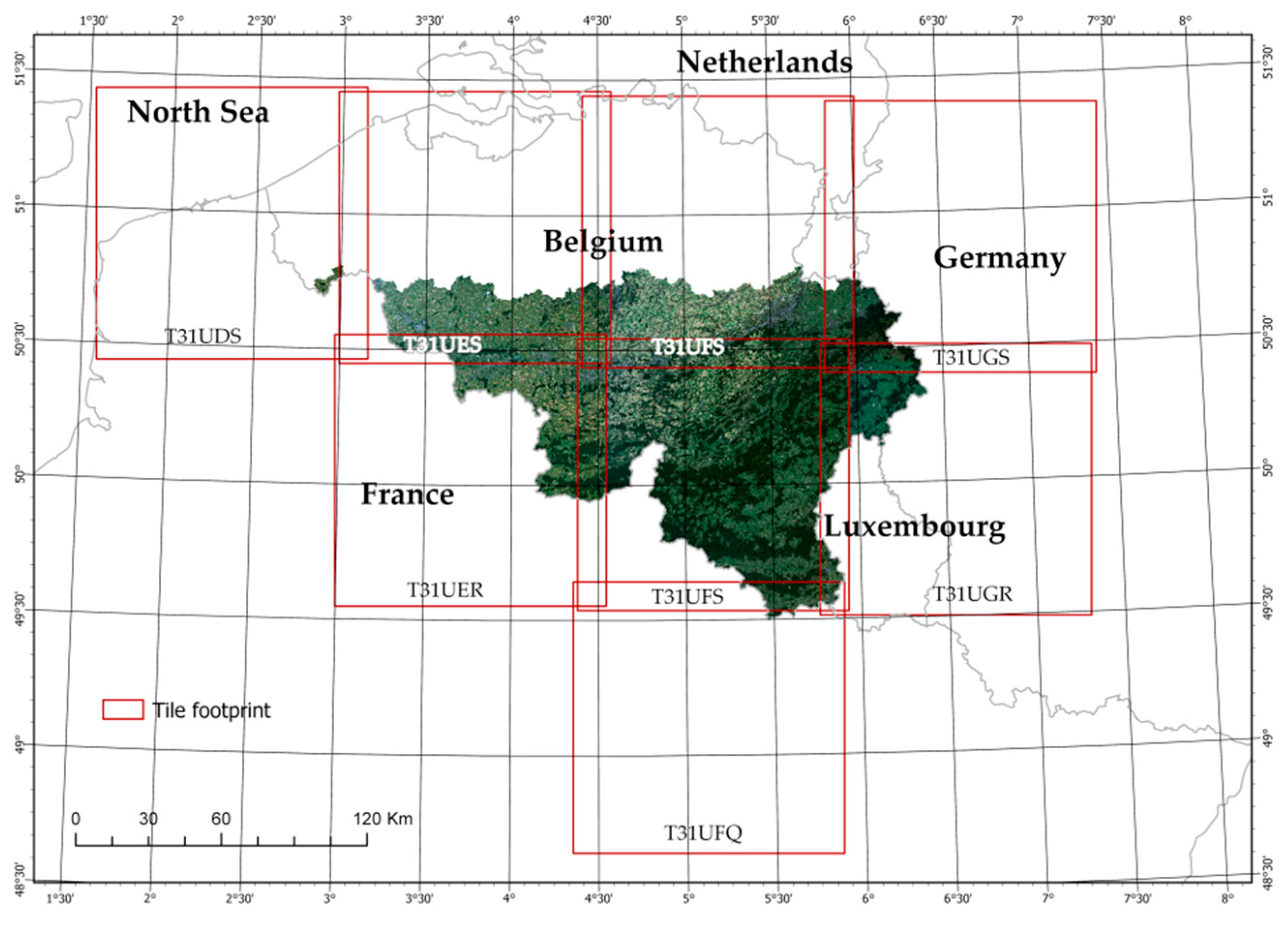
Figure 1.
Tiles arrangement allowing the realization of the six mosaics of Sentinel-2 in Wallonia, Belgium. Eight tiles (T31UDS, T31UES, T31UFS, T31UGS, T31UER, T31UFS, T31UGR, and T31UFQ) were used to produce six mosaics. The data spanned from December 2016 (winter 2016 mosaic), March to May 2016 (spring 2016 mosaic), July to September 2016 (summer 2016 mosaic), February to March 2018 (winter 2018 mosaic), May 2018 (spring 2018 mosaic) and, June to August 2018 (summer 2018 mosaic). These periods depended mainly on the availability of usable Sentinel-2 images.

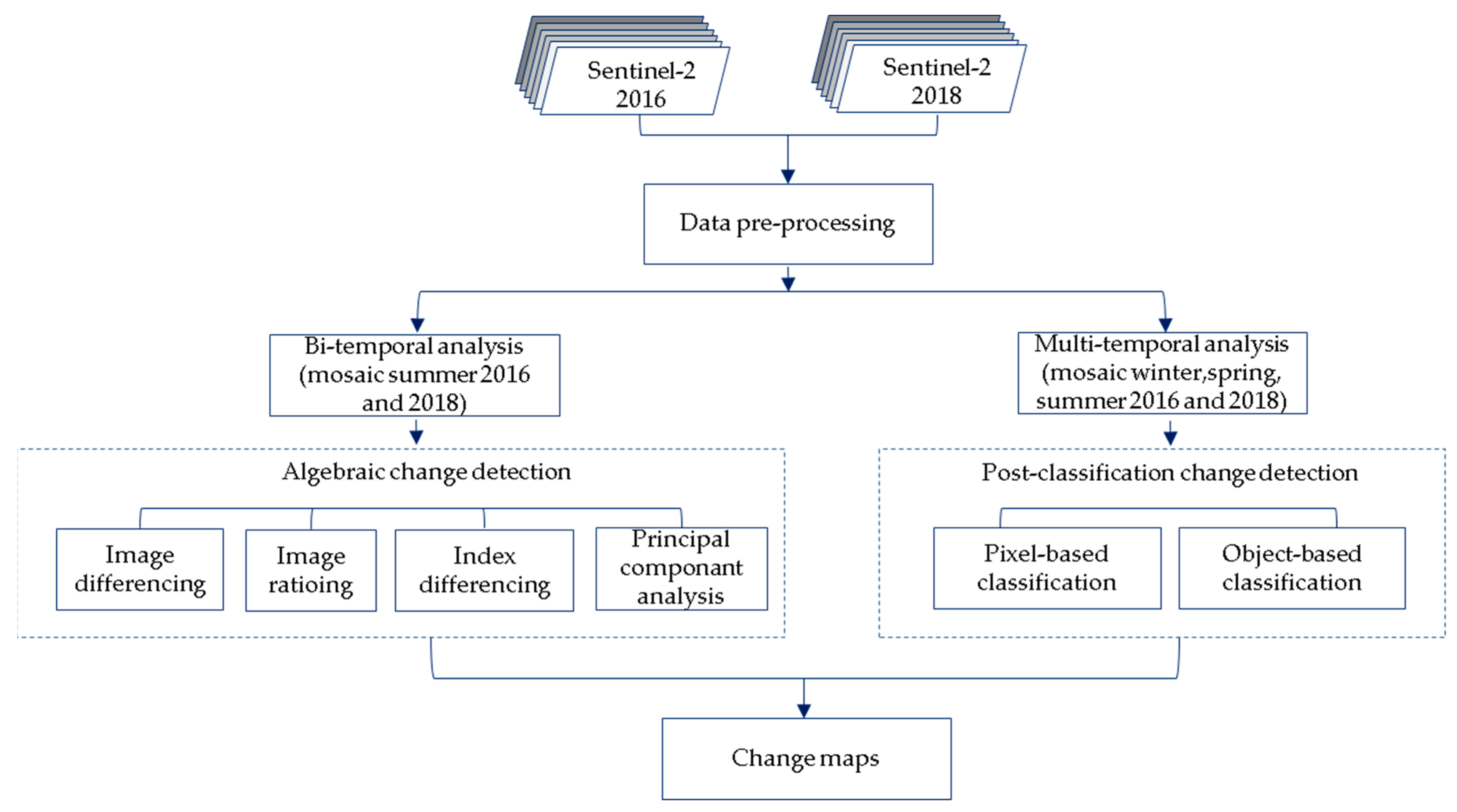
Figure 2.
Workflow of the change detection analysis. Two sets of Sentinel-2 data have been pre-processed to produce cloudless and snowless mosaics from winter, spring and summer season of 2016 and 2018 following the procedure described in reference [26]. Then, two approaches of change detection analysis have been tested: (1) algebraic (image differencing, image ratioing, index differencing, principal component analysis) and, (2) post-classification (pixel-based classification and object-based classification). Finally, change maps have been generated for each method.

Figure 3.
Distribution of the 2141 reference points across Wallonia. This dataset is based on LUCAS database and WAW layer.
Figure 3.
Distribution of the 2141 reference points across Wallonia. This dataset is based on LUCAS database and WAW layer.

Figure 4.
Sentinel-2 images from 2016 and 2018 showing an area of interest. The boundary of the location of the observed changes are delimitated by black polygons.
Figure 4.
Sentinel-2 images from 2016 and 2018 showing an area of interest. The boundary of the location of the observed changes are delimitated by black polygons.

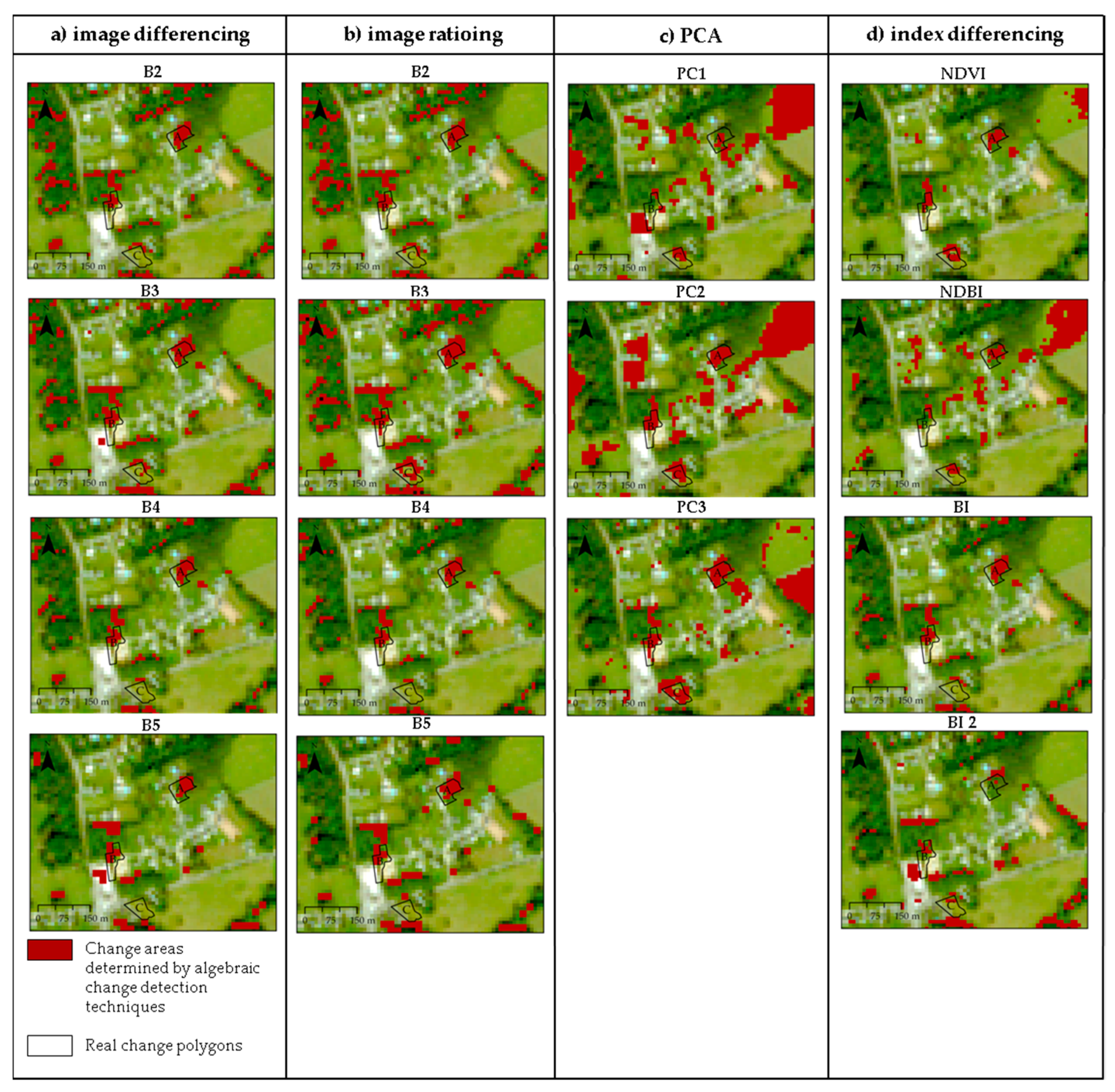
Figure 5.
Algebraic change maps: (a) image differencing; (b) image ratioing; (c) principal component analysis (PCA); (d) index differencing. Thresholds of the binary maps have been made through visual observation. The background image is the Sentinel-2 image from the year 2016. The black polygons are delimiting the location of the observed change areas and the red pixels correspond to the change areas determined by the pre-classification techniques.

Figure 6.
Post-classification analysis: object-based classification results. The first panel shows the aerial orthophotography of 2016 and 2018. Three areas of change are delimited by black polygons. The second panel shows the object-based classification of both years. The last panel is the change map of the object-based classification. The red pixels are delimiting the areas of change according to the classification, and the black polygons the location of observed changed areas.

Figure 7.
Post-classification analysis: pixel-based classification results. The first panel shows the aerial orthophotography of 2016 and 2018. Three areas of change are delimited by black polygons. The second panel shows the pixel-based classification of both years. The last panel is the change map of the pixel-based classification. The red pixels are delimiting the areas of change according to the classification, and the black polygons the location of observed changed areas.

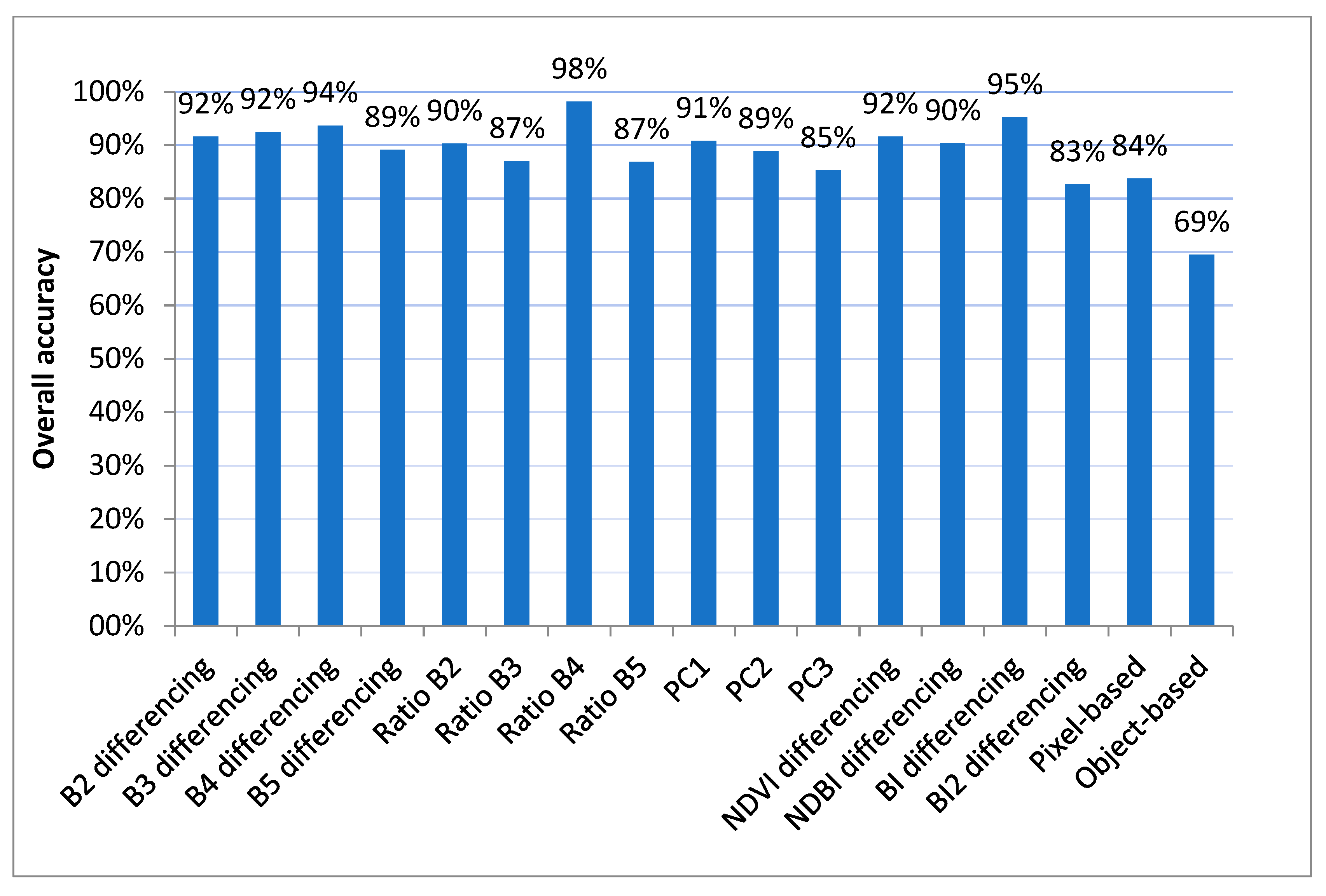
Figure 8.
Overall accuracy (%) of the algebraic and post-classification techniques. Ratio B4 (98%), BI differencing (95%) and B4 differencing (94%) present the highest overall accuracy.
Figure 8.
Overall accuracy (%) of the algebraic and post-classification techniques. Ratio B4 (98%), BI differencing (95%) and B4 differencing (94%) present the highest overall accuracy.

Figure 9.
Omission errors of the algebraic and post-classification techniques. The Object-based change detection technique has the highest omission errors (652). Ratio B4 has the lowest omission errors (32).
Figure 9.
Omission errors of the algebraic and post-classification techniques. The Object-based change detection technique has the highest omission errors (652). Ratio B4 has the lowest omission errors (32).

Figure 10.
Commision errors of the algebraic and post-classification techniques. The Object-based change detection technique has the lowest commission errors (2).
Figure 10.
Commision errors of the algebraic and post-classification techniques. The Object-based change detection technique has the lowest commission errors (2).

Table 1.
Principal component analysis of the mosaic of summer 2016. This mosaic contains 10 bands (B2, B3, B4, B5, B6, B7, B8, B8A, B11, B12).
Table 1.
Principal component analysis of the mosaic of summer 2016. This mosaic contains 10 bands (B2, B3, B4, B5, B6, B7, B8, B8A, B11, B12).
| Band | Eigenvalue | Percent of Eigenvalues | Accumulative of Eigenvalues |
|---|---|---|---|
| B2 | 4028,976.59 | 70.78 | 70.78 |
| B3 | 1386,233.87 | 24.35 | 95.13 |
| B4 | 135,458.47 | 2.38 | 97.51 |
| B5 | 71,961.32 | 1.26 | 98.78 |
| B6 | 22,233.99 | 0.39 | 99.17 |
| B7 | 20,524.41 | 0.36 | 99.53 |
| B8 | 13,311.03 | 0.23 | 99.76 |
| B8A | 6197.79 | 0.11 | 99.87 |
| B11 | 5146.81 | 0.09 | 99.96 |
| B12 | 2213.52 | 0.04 | 100.00 |
Table 2.
Land cover accounts of Wallonia derived from CLC 2006–2018 (https://land.copernicus.eu/pan-european/corine-land-cover).
Table 2.
Land cover accounts of Wallonia derived from CLC 2006–2018 (https://land.copernicus.eu/pan-european/corine-land-cover).
| Artificial Surfaces | Agricultural Areas | Forest and Semi Natural Areas | Wetlands | Waterbodies | |
|---|---|---|---|---|---|
| CLC 2018 (km2) | 2563 | 9007 | 5226 | 63 | 45 |
| Change 2012–2018 (%) | 0.51 | −0.13 | −0.12 | 8.81 | 0.22 |
| CLC 2012 (km2) | 2551 | 9019 | 5232 | 58 | 45 |
| Change 2006–2012 (%) | 1.41 | −0.42 | −0.01 | 4.95 | 0.18 |
| CLC 2006 (km2) | 2515 | 9057 | 5233 | 56 | 45 |
Table 3.
Statistics of reference points per land categories for the year 2016 and 2018.
| Land Categories | Points 2016 | Points 2018 | Change (%) |
|---|---|---|---|
| Forest land | 721 | 720 | −0.14% |
| Cropland | 535 | 535 | 0.00% |
| Grassland | 487 | 485 | −0.41% |
| Wetland | 150 | 150 | 0.00% |
| Settlement | 248 | 251 | 1.21% |
| Total | 2141 | 2141 | 0.37% |
Table 4.
Percentage of changed and unchanged areas in Wallonia associated with pre-classification CD techniques.
Table 4.
Percentage of changed and unchanged areas in Wallonia associated with pre-classification CD techniques.
| Image Differencing | Image Ratioing | PCA | Index Differencing | ||||||
|---|---|---|---|---|---|---|---|---|---|
| No Change | Change | No Change | Change | No Change | Change | No Change | Change | ||
| B2 | 92.90 | 7.10 | 91.63 | 8.37 | 88.69 | 11.31 | 92.54 | 7.46 | NDVI |
| B3 | 92.21 | 7.79 | 88.49 | 11.51 | 88.22 | 11.78 | 90.73 | 9.27 | NDBI |
| B4 | 93.60 | 6.40 | 98.40 | 1.60 | 84.24 | 15.76 | 95.27 | 4.73 | BI |
| B5 | 91.15 | 8.85 | 89.99 | 10.01 | / | / | 85.12 | 14.88 | BI2 |
Table 5.
Percentage of changed and unchanged areas in Wallonia associated with object-based classification, overall accuracy (OA) of each classification and the associated errors in percentage.
Table 5.
Percentage of changed and unchanged areas in Wallonia associated with object-based classification, overall accuracy (OA) of each classification and the associated errors in percentage.
| Object-Based Change Map | ||
| % | ||
| No change | 67.22 | |
| Change | 32.78 | |
| OA% | Errors% | |
| Classification 2016 | 84.65 | 15.35 |
| Classification 2018 | 76.56 | 23.44 |
| Total | / | 38.79 |
Table 6.
Percentage of changed and unchanged areas in Wallonia associated with pixel-based classification, overall accuracy (OA) of each classification and the associated errors in percentage.
Table 6.
Percentage of changed and unchanged areas in Wallonia associated with pixel-based classification, overall accuracy (OA) of each classification and the associated errors in percentage.
| Pixel-Based Change Map | ||
| % | ||
| No change | 83.40 | |
| Change | 16.60 | |
| OA% | Errors% | |
| Classification 2016 | 91.90 | 8.10 |
| Classification 2018 | 91.70 | 8.30 |
| Total | / | 16.40 |
Table 7.
Error matrix reported in terms of estimated area proportions (km2).
| Pixel-Based Classification 2018 | |||||||
|---|---|---|---|---|---|---|---|
| Forest Land | Cropland | Grassland | Wetland | Settlement | ∑ | ||
| Pixel-based classification 2016 | Forest land | 3588.93 | 78.10 | 0.08 | 141.09 | 281.28 | 4089.47 |
| Cropland | 147.20 | 5110.42 | 2.11 | 349.63 | 114.16 | 5723.52 | |
| Grassland | 1.57 | 4.18 | 50.04 | 18.80 | 0.00 | 74.60 | |
| Wetland | 321.13 | 177.23 | 2.28 | 1761.23 | 294.53 | 2556.41 | |
| Settlement | 737.48 | 58.76 | 0.00 | 306.24 | 3347.15 | 4449.63 | |
| ∑ | 4796.31 | 5428.69 | 54.51 | 2576.97 | 4037.12 | 16,893.62 | |
Table 8.
Percentage of changes for the three validation datasets: CLC, AAP and reference points for Wallonia. The cropland category of CLC in this table corresponds to agricultural area in the CLC nomenclature. This includes both agricultural and pastoral lands. The wetland category of CLC in this table corresponds to wetlands and water bodies in the CLC nomenclature.
| CORINE Land Cover (CLC) | Anonymous Agricultural Plot (AAP) | Reference Points | |||||||
|---|---|---|---|---|---|---|---|---|---|
| 2012 (km2) | 2018 (km2) | Change (%) | 2016 (km2) | 2018 (km2) | Change (%) | 2016 (Points) | 2018 (Points) | Change (%) | |
| Forest land | 5232.2 | 5225.96 | 0.51 | N/A | N/A | N/A | 721 | 720 | −0.14 |
| Cropland | 9018.94 | 9006.99 | −0.13 | 3898.40 | 3905.43 | 0.18 | 535 | 535 | |
| Grassland | 4221.08 | 4328.54 | 2.55 | 487 | 485 | −0.41 | |||
| Wetland | 103.25 | 108.49 | 5.08 | N/A | N/A | N/A | 150 | 150 | |
| Settlement | 2550.54 | 2563.49 | 0.51 | N/A | N/A | N/A | 248 | 251 | 1.21 |
Table 9.
Chi squared test for evaluating the statistical significance between pixel-based classification and object-based classification [45].
Table 9.
Chi squared test for evaluating the statistical significance between pixel-based classification and object-based classification [45].
| Pixel-Based Classification | X2 | ||||
|---|---|---|---|---|---|
| Allocation | Correct | Incorrect | ∑ | 910.7201 | |
| Object-based classification | Correct | 1280 | 207 | 1487 | |
| Incorrect | 512 | 142 | 654 | ||
| ∑ | 1792 | 349 | 2141 | ||
Publisher’s Note: MDPI stays neutral with regard to jurisdictional claims in published maps and institutional affiliations. |
© 2021 by the authors. Licensee MDPI, Basel, Switzerland. This article is an open access article distributed under the terms and conditions of the Creative Commons Attribution (CC BY) license (http://creativecommons.org/licenses/by/4.0/).
Share and Cite
MDPI and ACS Style
Close, O.; Petit, S.; Beaumont, B.; Hallot, E. Evaluating the Potentiality of Sentinel-2 for Change Detection Analysis Associated to LULUCF in Wallonia, Belgium. Land 2021, 10, 55. https://doi.org/10.3390/land10010055
AMA Style
Close O, Petit S, Beaumont B, Hallot E. Evaluating the Potentiality of Sentinel-2 for Change Detection Analysis Associated to LULUCF in Wallonia, Belgium. Land. 2021; 10(1):55. https://doi.org/10.3390/land10010055
Chicago/Turabian StyleClose, Odile, Sophie Petit, Benjamin Beaumont, and Eric Hallot. 2021. "Evaluating the Potentiality of Sentinel-2 for Change Detection Analysis Associated to LULUCF in Wallonia, Belgium" Land 10, no. 1: 55. https://doi.org/10.3390/land10010055
Note that from the first issue of 2016, this journal uses article numbers instead of page numbers. See further details here.