
The Spatial Distribution and Prediction of Soil Heavy Metals Based on Measured Samples and Multi-Spectral Images in Tai Lake of China


1
School of Geoscience and Technology, Zhengzhou University, Zhengzhou 450001, China
2
School of Politics and Public Administration, Zhengzhou University, Zhengzhou 450001, China
3
Henan Geological Survey Institute, Zhengzhou 450001, China
4
Contemporary Capitalism Research Center, Zhengzhou University, Zhengzhou 450001, China
5
School of Land Science and Technology, China University of Geosciences, Beijing 100083, China
*
Author to whom correspondence should be addressed.
Land 2021, 10(11), 1227; https://doi.org/10.3390/land10111227
Submission received: 13 October 2021
/
Revised: 2 November 2021
/
Accepted: 8 November 2021
/
Published: 11 November 2021
(This article belongs to the Topic Climate Change and Environmental Sustainability)
Abstract
:Soil is an important natural resource. The excessive amount of heavy metals in soil can harm and threaten human health. Therefore, monitoring of soil heavy metal content is urgent. Monitoring soil heavy metals by traditional methods requires many human and material resources. Remote sensing has shown advantages in the field of monitoring heavy metals. Based on 971 heavy metal samples and Sentinel-2 multi-spectral images in Tai Lake, China, we analyzed the correlation between six heavy metals (Cd, Hg, As, Pb, Cu, Zn) and spectral factors, and selected As and Hg as the input factors of inversion model. The correlation coefficient of the best model of As was 0.53 (p < 0.01), and of Hg was 0.318 (p < 0.01). We used the methods of partial least squares regression (PLSR) and back propagation neural network (BPNN) to establish inversion models with different combinations of spectral factors by using 649 measured samples. In addition, 322 measured samples were used for accuracy evaluation. Compared with the PLSR model, the BP neural network builds the model with higher accuracy, and B1-B4 combined with LnB1-LnB4 builds the model with the highest accuracy. The accuracy of the best model was verified, with an average error of 19% for As and 45% for Hg. Analyzing the spatial distribution of heavy metals by using the interpolation method of Kriging and IDW. The overall distribution trend of the two interpolations is similar. The concentration of As elements tends to increase from north to south, and the relatively high value of Hg elements is distributed in the east and west of the study area. The factories in the study area are distributed along rivers and lakes, which is consistent with the spatial distribution of heavy metal enrichment areas. The relatively high-value areas of heavy metal elements are related to the distribution of metal products factories, refractory porcelain factories, tile factories, factories and mining enterprises, etc., indicating that factory pollution is the main reason for the enrichment of heavy metals.
1. Introduction
Soil is not only an important natural resource but also an environment which human beings depend on. With the rapid development of the economy, human activities such as mineral resources exploitation, metal processing, smelting, chemical production, factory drainage, and sewage irrigation, the content of soil heavy metals has increased and put great pressure on human production, life, and soil resources [1,2]. Excessive soil heavy metal content could cause irreparable damage to human health. For instance, acute and chronic As exposure could lead to cardiovascular disorders, while excessive Pb can damage the central nervous system, leading to headache, insomnia, and memory loss [3,4]. Heavy metal pollution is exacerbated by metal based industrial activities, and heavy metals can enter the human body through contaminated food, inhaled through the atmosphere, drunk via contaminated water, through skin contact from agriculture, etc. The toxicity of heavy metals can increase the incidence of many human cancers. There is a need for regular testing and control of heavy metals to protect human health [5,6]. Therefore, the monitoring of soil heavy metal content is urgent.
At present, the traditional monitoring of soil heavy metals is a chemical analysis method, which has high observation accuracy, but is only suitable for small-scale local areas. Wide-scale monitoring of soil heavy metal content requires a lot of human and material resources [7]. Remote sensing technology has the characteristics of fast monitoring speed, wide range, short cycle, non-destructiveness, etc. It overcomes the shortcomings of traditional monitoring methods and has been widely used in the field of soil monitoring [8,9,10,11]. Kemper and Sommer (2002) predicted the content of six heavy metals using multiple linear regression models and artificial neural network models. The study proved the feasibility of using multiple linear regression models and artificial neural network models to establish reliable chemical metrological models [7]. Luce et al. (2017) demonstrated that it is possible to predict a smaller degree of water-soluble soil heavy metals by using the partial least squares model (PLSR) in visible near-infrared spectroscopy [12]. The methods of univariable regression and principal component analysis were used to predict the concentration of Hg and the best model (R = 0.69, RMSE = 0.15) proved that it was feasible to predict Hg in agriculture by reflection spectroscopy [13]. Yan et al. (2009) carried out a differential transformation, baseline correction, and other pretreatments of hyperspectral data to establish a PLSR of heavy metal elements and selected the best model to invert the content of As, Fe, and Cu elements [14]. Pyo et al. (2020) used CNN (convolutional neural network) learning models to predict the concentrations of Cu and Pb, and used spectral data to establish machine learning models to invert heavy metal concentrations [15]. Liu et al. (2019) established the PSO-BPNN model to invert the content of Cd, Hg, and As elements, which improved the prediction accuracy of the heavy metal inversion model greatly, and indicated that machine learning methods had great potential to estimate the content of soil heavy metals accurately [16]. Choe et al. (2009) used heavy metals to establish EMLR (stepwise multiple linear regression) and SMLR (enter multiple linear regression) prediction models based on the spectral response of heavy metals to visible near-infrared bands and predicted the possibility of visible near-infrared bands in the spatial distribution prediction of heavy metals [17]. Shi et al. (2007) used the method of Kriging interpolation to describe the spatial distribution of six heavy metals in Changxing County, Zhejiang Province and assessed the risk of heavy metal pollution [18]. Mapping the distribution of heavy metal concentrations in the study area provides a more visual and detailed understanding of the spatial distribution between heavy metal concentrations and industrial activities, which can be applied to prevent soil contamination and, in some cases, to use microorganisms to cleanse the soil of heavy metals and scientifically restore soil health [19,20].
In summary, most of the areas of research for remote sensing inversion of soil heavy metals have focused on mining areas and river coasts, while the inversion of heavy metals content in the Tai Lake is rarely involved. Tai Lake is located near the Yangtze River Delta region, one of the most economically developed regions in China, and its urbanization and industrialization have accelerated the accumulation of heavy metals in the soil, posing a potential hazard to the soil. Based on fieldwork, the study area is relatively well-developed in terms of industry, especially pottery production. Heavy metal content monitoring can measure the impact of industrial activities on the soil, which provides important information for scientific soil protection. Multispectral data has the advantages of low cost and availability. This study used a Sentinel-2 satellite image, and the image has a spatial resolution of up to 10 m in the B2, B3, B4, and B8 bands. The spectral data of Sentinel-2 is mathematically transformed to reduce the spectral characteristics of non-heavy metals and highlight the spectral characteristics of soil heavy metals. The selection of the model affects the accuracy of heavy metal prediction, and partial least square regression (PLSR) and back propagation neural network (BPNN) models are used as soil heavy metal content prediction models [21].
In this study, we analyze spatial distribution characteristics of heavy metals in the study area based on 971 measured samples in Tai Lake, Jiangsu Province, including Cd, Hg, As, Pb, Cu, and Zn, and analyzed the correlation between spectral factors and the six heavy metals. We selected the target heavy metals with high correlation and established inversion models by combining spectral data from Sentinel-2 images. The main research contents are as following: (1) To analyze the distribution characteristic of six heavy metals and compare with the background value of heavy metals in Jiangsu Province and the national soil pollution screening value. (2) To analyze the correlation between heavy metals and Sentinel 2 spectral factors, and select the target heavy metals with high correlation as the input factors of the inversion model. (3) To establish the inversion model by using the method of partial least squares model (PLSR) and back propagation neural network model (BPNN), and evaluate the accuracy of the model. (4) To predict the content of heavy metals by combining with the optimal inversion model, analyzing the spatial distribution characteristics of the target heavy metals in the region, and the relationship between high-value areas of heavy metals and factory distribution.
2. Materials and Methods
2.1. Sample Collection and Chemical Analysis
As shown in Figure 1, the research area is located in Tai Lake, Jiangsu Province. Soil sampling was carried out near Tai Lake. There are six soil types in this study region, including Anthrosols, Ferralisols, Luvisols, Skeletol primitive soils, Dark Semi-hydromorphic soils, and Hydromorphic soil. Most soil samples (783, 80.6%) were distributed in Anthrosols, followed by Ferralisols (101, 10.4%), Luvisols (23, 2.3%), Skeletol primitive soils (18, 1.8%), Dark Semi-hydromorphic soils (7, 0.7%), and Hydromorphic soils (0, 0%).
According to the grid layout, a total of 971 sampling points were collected during 2010–2011, included 854 farmland samples, 98 dryland samples, and 11 paddy land samples, and accurate longitude and latitude coordinates were recorded with GPS. Overall, most of the sampling points were distributed on the farmland of the research area. To ensure that the modeling set and the validation set represented the statistical characteristics of the sample, we used the random function to randomly extract a 2:1 scale from the 971 soil samples, using 649 as the modeling set and the remaining 322 as the validation set.
During the sampling process, the soil sampling depth was 0~20 cm. To avoid the effects of soil which were transferred from somewhere else or disturbed by some human activities, as well as newly disturbed soil layers, five-point sampling methods were used to remove surface debris and gravel in the soil, retaining 1kg of polyethylene self-capsuling soil sample for each collected sample. In this study, the contents of six heavy metals, Cd, Hg, As, Pb, Cu, and Zn, were determined. Cd and Pb in soil were determined by graphite furnace atomic absorption spectrometry (Optima 2100DV, Perkin Elmer, USA), Cu and Zn in soil were determined by flame atomic absorption spectrometry (Optima 2100DV, Perkin Elmer, USA), Zn, Hg, and As in soil were determined by atomic fluorescence spectrometry (Primus-II, Rigaku Corporation, Japan), and Cr in soil was additionally determined by inductively coupled plasma atomic emission spectrometry (Optima 2100DV, Perkin Elmer, USA). The process of measuring heavy metal concentration is consistent with Hou [22].
2.2. Image Data Source and Processing
The study utilized cloud-free high-quality sentinel-2 multispectral images (2015.12) from the United States Geological Survey (https://earthexplorer.usgs.gov/ accessed on 7 November 2021). Sentinel 2 is a high-resolution multispectral imaging satellite carrying a multispectral imager (MSI) for land monitoring, providing images of vegetation, soil, and water cover, inland waterways and coastal areas, and emergency relief services. Given that most crops in the farmland have been harvested and the surface vegetation is sparse in winter, the image data chosen was 25 December 2015. ENVI 5.3 radiated Sentinel 2 satellite imagery, atmospheric correction, and other pretreatments were used to obtain the actual reflectance of the surface. Because the imaging of the study area contains plant spectral information and the spectral characteristics of heavy metals in the soil were relatively weak, to eliminate soil background noise and enhance the information related to heavy metals in the spectral band, this study considered the results of spectral bands, their number transformation, and NDVI factors as spectral factors to be modeled [23,24].
2.3. Model and Method
2.3.1. Selection of Modeling Factors
The selection of modeling factors is determined by the correlation between the spectral band and heavy metal content, where Ln represents the logarithmic operation on the band. The correlation coefficient represents the ability of the spectral characteristic to explain the content of heavy metals. The higher the correlation coefficient, the stronger the interpretation ability. By calculating the correlation coefficient between each spectral factor and the soil heavy metal content, the target heavy metal and spectral factor variables were selected as the input variables of the model.
2.3.2. Model Method
The partial least squares regression method was used to establish the relationship between spectra and soil variables. The partial least squares method is the most widely used method in multivariate correction and is based on a latent variable decomposition of two blocks of variables, containing spectral data and soil properties, respectively. The purpose of the method is to identify a small number of latent factors that can be effectively predicted and used. The model of PLSR (partial least square regression) has the advantages of principal component analysis, typical correlation analysis, and ordinary multivariate linear regression, which overcomes multiple linear correlations between independent variables and makes the model more stable and accurate [25].
BPNN (back propagation neural network) is a kind of artificial neural network. It is based on the error reverse propagation algorithm. The learning process consists of the forward propagation of the input signal and the reverse propagation of the error. The training process includes constantly adjusting the connection weight until the output error reaches the required standard [26]. To build the model, a 3-layer neuron network is used, including the input layer, hidden layer, and output layer; the Sigmoid transfer function is used for the hidden layer neurons and the Purelin function is used for the output layer. In this paper, the previously selected modeling factors were used as the learning input samples of the network model, and the corresponding heavy metal content was used as the expected output of the learning matrix. By repeatedly learning and training the correspondence between input and output sequences, and continuously adjusting the input and hidden layers of the network model, the mapping relationship between remote sensing reflectance and heavy metal content can be established [21].
2.3.3. Spatial Interpolation Method
We used the best inversion model to estimate the content of heavy metal of each pixel by combining the spectral band, and then used the Kriging and IDW interpolation to obtain the content of heavy metal for the whole study region. Kriging interpolation is the core of local statistical interpolation. This interpolation method is based on the spatial characteristics of heavy metal content to determine the weight of the sampling point on the predicted value. It gives an overall optimal unbiased estimate of the content of heavy metals in the region. Kriging interpolation is used to interpolate the research area based on the measured sample data [27].
IDW stands for Inverse Distance Weight Interpolation. IDW interpolation is an accurate interpolation method, which determines weighting according to the distance impact. The more significant the distance weighting coefficient, the more extensive the impact range of the local maximum, and the larger the prediction range of the contaminated area [28,29].
2.3.4. Model Evaluation Method
The partial least squares regression model and BP neural network model of the target heavy metals and spectral factors were established by MATLAB R2020a. The R correlation coefficient and the root mean square error of RMSE were used as the evaluation parameters of the model [30]. The closer R is to 1, the more stable the model is and the better the fit is. The RMSE indicates the model’s predictive power. The larger the coefficient of determination R of the model, the smaller the root mean square error RMSE, and the more accurate the model inversion is judged. According to the R correlation coefficient, screening the target heavy metal and spectral factors allows the choice of optimal inversion model of the target heavy metal. The error judgment model accuracy is verified between the measured value of the sample point and the best model inversion value.
The following parameters are used to evaluate the accuracy of the model:
where n is the number of samples, Yi represents the real value of heavy metal content of the samples, and Xi is the predicted value of heavy metal content of the ith samples. Xi represents the real value of the band of the ith samples, and i is the predicted value of the band of the ith samples.
3. Results and Discussion
3.1. Analysis of Heavy Metal Characteristics
Statistical analysis of six heavy metals in 971 soil samples in the study area showed in Table 1. The most extensive content of heavy metals was Cu, with a maximum of 593 mg/kg and an average of 29.348 mg/kg. The smallest content of heavy metals was Hg with a minimum value of only 0.018 mg/kg, and an average value of 0.132 mg/kg. Comparison of the content of heavy metal with the background values of Jiangsu Province showed the average values of Hg and As were smaller than that of Jiangsu Province, while the average content of the other four heavy metals (Cd, Pb, Cu, Zn), exceeded the background value of Jiangsu Province, indicating that the content of heavy metal elements in the soil had been affected by human activities.
Measured distribution maps of heavy metal content were made by ArcGIS10.5 software. Compared with the national soil pollution standards [31], the average value of all six heavy metals content was less than the national soil pollution standard; e.g., the average value of Hg element was only one-third of the national standard value. The maximum value of As element was also lower than the national standard value, indicating that the soil quality was sufficient to meet the needs of agricultural production and human activities.
The coefficient of variation is the ratio of the standard deviation from the average value of the original data, which was used to analyze the discreteness of the data. The larger the value, the greater the variation of the data. The variation of the content of six heavy metals in the surface soil was sequential: Cd > Cu > Hg > Zn > Pb > As. It was generally recognized that the coefficient of variation reflects the degree of dispersion. When the coefficient of variation is between 10% and 100%, medium variability is indicated, so the content of all six types of heavy metals in the soil was of medium variability. The moderate variation with a large coefficient of variation indicates that the internal structure of the measured data may show a strong moderate variation influenced by human activities and other factors.
Figure 2 shows that different heavy metals had different spatial distribution characteristics. The content of Cd in the western part of the research area was relatively high, and the overall distribution increased from east to west; the content of Hg was higher in the eastern and western parts of the study area; the high value of As was mainly distributed in the south of the study area; the content of Pb was relatively high in the eastern and western parts of the research area; the relative height of Cu was mainly distributed in the northwest of the research area; and the relatively high value of Zn was distributed primarily on the western and northeast parts of the research area.
3.2. Determine the Factors of Modeling
Pearson correlation coefficient was used to evaluate the correlation between heavy metal content and spectral factors, and the results are shown in Table 2.
As shown in Table 2, it was concluded that the As correlation coefficient was highest in R (0.3–0.5), followed by Hg (0.2–0.3), and the remaining four heavy metals (Cd, Pb, Cu, Zn) were low (R < 0.1). Therefore, the relatively relevant As and Hg elements were selected as the target heavy metals. The correlation between As, Hg, and spectral factors was analyzed, and is shown in Table 3.
From Table 3, the correlations of target heavy metals with B6~B8 and B8A were lower than those with B1~B5 bands. The correlations between the target heavy metals and the logarithmic operation of the spectral factors were all improved. The spectral factors were negatively correlated with As and positively correlated with Hg, and the correlations were all at the p < 0.01 confidence level. The correlation coefficient between the target heavy metal and lnB1~B4 was higher than that with spectral reflectivity B1~B4, which was also related to NDVI. The results showed that the content of heavy metals in the study area had a good correlation with spectral factors B1~B4 and lnB1~lnB4, indicating that spectral factors B1~B4, LnB1~LnB4, and NDVI could be used to predict the soil heavy metal content and spatial distribution.
3.3. Model Accuracy Evaluation
A total of 649 soil samples were randomly extracted from 971 soil samples on a 2:1 scale as modeling sets. PLSR and BPNN models were established with target heavy metals and spectral factors as model input variables.
As shown in Table 4, the results showed that for the modeling set of As elements based on the PLSR model, R was between 0.431 and 0.462, and RMSE was between 1.943 and 1.976 (see Table 4); the verification set was between 0.498~0.526, and RMSE was between 2.007 to 2.045. The correlation coefficient difference based on the original band modeling and adding the NDVI factor model was only 0.001, which was very small: the NDVI factor cannot significantly improve the accuracy. For the Hg element modeling set, R was between 0.257 and 0.268, and RMSE was between 0.062 and 0.066; the verification set was between 0.149 and 0.161, and RMSE was between 0.105 and 0.191. Similarly, NDVI cannot significantly improve the accuracy of mercury elements. For the PLSR prediction models of As and Hg elements, both are logarithmically calculated by spectral factors as input variables with higher model accuracy than spectral bands. The target heavy metal prediction model established by spectral factors LnB1~LnB4 and NDVI had the highest accuracy.
As shown in Table 5, based on the BP model, for the As modeling set, R ranged from 0.482 to 0.530, and RMSE was 1.860~1.909; for the verification set, R was 0.467~0.532, and RMSE was 1.999 to 2.094. For the Hg element modeling set, R was between 0.263 and 0.318, and RMSE was between 0.061 and 0.062; the verification set was between 0.149 and 0.186, and RMSE was between 0.105 and 0.288. Compared with the five PLSR models, the correlation between the BP model of the target heavy metal content was correspondingly improved, and the accuracy was relatively high.
The larger the decision coefficient and the smaller the root mean square error, the more stable and accurate the model is. It can be concluded that the model with the highest accuracy of As was the BP model established by the B1~B4 spectral factor, R = 0.530; the model with the highest accuracy of Hg was the BP model based on B1~B4 and NDVI spectral characteristic, R = 0.318. For the As element, the relative error of modeling was 0.201, and for the Hg element, the relative error was 0.498. The PLSR model and BP model can establish the target metal content and spectral reflection factor to predict the metal content of the study area. It can be shown from the evaluation parameters of the model that the modeling and prediction ability of the BP model was high, and it had a good interpretation ability of the target soil heavy metals.
Based on the verification set, the two models were accurately verified. The model was inverted and the predicted value of the target heavy metal was obtained. The scatter plot was drawn by the measured and predicted values of the verification set. As shown in the following Figure 3, As elements were generally distributed near the 1:1 trend line (0.478), while for Hg elements, the measured and predicted value distributions were discrete (0.452) compared with the distribution of As element. This showed that the BP neural network model had a good interpretation ability for the predicted value of heavy metals. The model can invert and study the content of heavy metals in the target area.
3.4. Spatial Distribution of Heavy Metal Content
The evaluation parameters R and RMSE of the model accuracy only reflected the difference between the measured and predicted value of the target heavy metal in the study area and the accuracy of establishing the model. Therefore, the spatial distribution of heavy metal content was mapped to analyze the spatial change trend of heavy metal content.
We used the method of Kriging interpolation and IDW interpolation to analyze the distribution of heavy metal content in the region. A prediction map of heavy metal content in the study area was obtained. The interpolation results are shown in Figure 4; comparative analysis of two spatial interpolation results, Kriging interpolation and IDW interpolation, show the spatial change trend of the heavy metal elements. As elements tended to increase from north to south, and Hg elements were concentrated in the eastern and western parts of the research area. IDW interpolation can highlight the local spatial characteristics of heavy metals more than Kriging interpolation. The northeast and northwest regions of the study all had local maximums, and for the Hg element, there were local maximums in the northeast of the research area. The reason for the high-value distribution in the study area was analyzed: the relatively high values of the four heavy metals were mainly distributed in the southwestern part of the eastern study area. The distribution law was consistent with the environment of the field sampling point.
3.5. Relationship between Heavy Metal Agglomerations and Factory Distribution
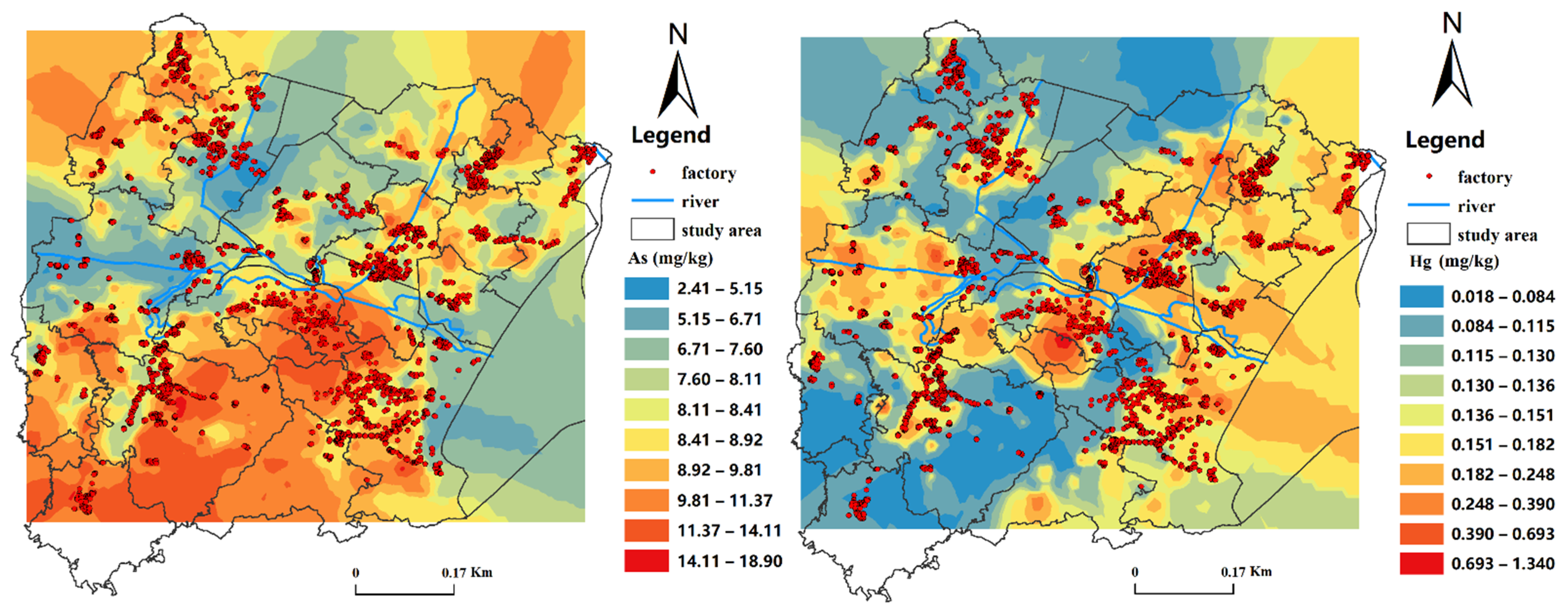
This study used Tuxin Earth to obtain the spatial distribution of factories in the study area. The factory distribution was shown in Figure 5. The factory was distributed at the river flow in the west of the research area, along the lake area in the southeast, and a small number in the south. Most of the factories in the research area were located along lakes and rivers. The high-value area of arsenic was partially consistent with the factory distribution along the lake area in the southeast of the research area, and a small number of high-value distributions in the northern part of the study area. The spatial interpolation distribution of mercury elements was relatively consistent with that of factories. The high value of mercury was distributed where rivers pass and along lakes. The high-value distribution law of heavy metals was consistent with the actual spatial distribution of factories.
4. Conclusions
This study focused on 971 measured samples of heavy metal elements in Tai Lake, Jiangsu Province, China. None of the six heavy metals exceeded the national soil pollution screening value, and the relatively high values of these four heavy metals (Cd, Pb, Cu, Zn) were mainly distributed in the factory area in the western and southeast in the study area. We analyzed the correlation between the heavy metal elements and the spectral factors from Sentinel-2 images and selected As, Hg, and B1-B4 band as the input elements of the inversion model with a high correlation. We established heavy metals inversion models based on the method of PLSR and BPNN, and the BPNN model had a higher inversion accuracy (R = 0.53 of As and R = 0.318 of Hg) than PLSR. We used the BPNN to invert the concentration of heavy metal for those no sample region, and the results were used to analyze the spatial difference by combining measured samples. The results indicated that the As element showed an increasing trend from north to south due to the distribution of dense factories in the southern region of the study area; the overall concentration of the Hg element was low, and the relatively high content area was distributed in the eastern and western parts of the research area. The high-value distribution law of heavy metals had a high relationship with the actual spatial distribution of factories, which suggested that human activities perhaps were the primary source of heavy metal. It is worth recommending that the relationship between human activities and the content of soil heavy metal should keep investigating in further work.
Author Contributions
Conceptualization, B.Q. and P.L.; methodology, H.Z.; software, H.Z.; validation, H.Z., B.Q. and P.L.; formal analysis, H.Z.; investigation, H.Z., B.Q. and P.L.; resources, P.L.; data curation, H.Z.; writing—original draft preparation, H.Z., B.Q. and P.L.; writing—review and editing, H.Z., B.Q. and P.L.; visualization, H.Z.; supervision, K.W.; project administration, B.Q. and P.L; funding acquisition, B.Q. and P.L. All authors have read and agreed to the published version of the manuscript.
Funding
This work was supported by the National Natural Science Foundation of China project (42001230, 41901078) and the China Postdoctoral Science Foundation (2020M672237). We would like to express our gratitude to Geological Survey of Jiangsu Province for the continuous support.
Institutional Review Board Statement
Not applicable.
Informed Consent Statement
Not applicable.
Data Availability Statement
The data presented in this study are available on request from the author.
Acknowledgments
This work was supported by the National Natural Science Foundation of China project (42001230, 41901078) and the China Postdoctoral Science Foundation (2020M672237). We would like to express our gratitude to Geological Survey of Jiangsu Province for the continuous support.
Conflicts of Interest
The authors declare no conflict of interest.
References
- Xu, X.; Zhao, Y.; Zhao, X.; Wang, Y.; Deng, W. Sources of heavy metal pollution in agricultural soils of a rapidly industrializing area in the Yangtze Delta of China. Ecotoxicol. Environ. 2014, 108, 161–167. [Google Scholar] [CrossRef]
- Yang, Q.; Li, Z.; Lu, X.; Duan, Q.; Huang, L.; Bi, J. A review of soil heavy metal pollution from industrial and agricultural re-gions in China: Pollution and risk assessment. Sci. Total Env. 2018, 642, 690–700. [Google Scholar] [CrossRef] [PubMed]
- Castelli, M.; Rossi, B.; Corsetti, F.; Mantovani, A.; Spera, G.; Lubrano, C.; Silvestroni, L.; Patriarca, M.; Chiodo, F.; Menditto, A. Levels of cadmium and lead in blood: An application of validated methods in a group of patients with endocrine/metabolic disorders from the Rome area. Microchem. J. 2005, 79, 349–355. [Google Scholar] [CrossRef]
- Jiang, H.-H.; Cai, L.-M.; Wen, H.-H.; Hu, G.-C.; Chen, L.-G.; Luo, J. An integrated approach to quantifying ecological and human health risks from different sources of soil heavy metals. Sci. Total Environ. 2020, 701, 134466. [Google Scholar] [CrossRef]
- Durowoju, O.S.; Ekosse, G.-I.E.; Odiyo, J.O. Occurrence and Health-Risk Assessment of Trace Metals in Geothermal Springs within Soutpansberg, Limpopo Province, South Africa. Int. J. Environ. Res. Public Health 2020, 17, 4438. [Google Scholar] [CrossRef]
- Briffa, J.; Sinagra, E.; Blundell, R. Heavy metal pollution in the environment and their toxicological effects on humans. Heliyon 2020, 6, e04691. [Google Scholar] [CrossRef]
- Kemper, T.; Sommer, S. Estimate of Heavy Metal Contamination in Soils after a Mining Accident Using Reflectance Spectroscopy. Environ. Sci. Technol. 2002, 36, 2742–2747. [Google Scholar] [CrossRef]
- Ge, Y.; Thomasson, J.A.; Sui, R. Remote Sensing of Soil Properties in Precision Agriculture: A Review. Front. Earth Sci. 2006, 5, 229–238. [Google Scholar] [CrossRef]
- Simoniello, T.; Lanfredi, M.; Liberti, M.; Coppola, R.; Macchiato, M. Estimation of vegetation cover resilience from satellite time series. Hydrol. Earth Syst. Sci. 2008, 12, 1053–1064. [Google Scholar] [CrossRef] [Green Version]
- Wang, F.; Gao, J.; Zha, Y. Hyperspectral sensing of heavy metals in soil and vegetation: Feasibility and challenges. ISPRS J. Photogramm. Remote Sens. 2018, 136, 73–84. [Google Scholar] [CrossRef]
- Hou, L.; Li, X.; Li, F. Hyperspectral-based Inversion of Heavy Metal Content in the Soil of Coal Mining Areas. J. Environ. Qual. 2019, 48, 57–63. [Google Scholar] [CrossRef] [PubMed] [Green Version]
- Luce, M.S.; Ziadi, N.; Gagnon, B.; Karam, A. Visible near infrared reflectance spectroscopy prediction of soil heavy metal concentrations in paper mill biosolid- and liming by-product-amended agricultural soils. Geoderma 2017, 288, 23–36. [Google Scholar] [CrossRef]
- Wu, Y.Z.; Chen, J.; Ji, J.; Tian, Q.; Wu, X. Feasibility of Reflectance Spectroscopy for the Assessment of Soil Mercury Contamination. Environ. Sci. Technol. 2005, 39, 873–878. [Google Scholar] [CrossRef]
- Yan, R.; Fang, Z.; Singh, A.; Jun, P.; Sheng, Q.; He, S. Estimation of As and Cu Contamination in Agricultural Soils Around a Mining Area by Reflectance Spectroscopy: A Case Study. Pedosphere 2009, 19, 719–726. [Google Scholar]
- Pyo, J.; Hong, S.; Kwon, Y.; Kim, M.; Cho, K. Estimation of heavy metals using deep neural network with visible and infrared spectroscopy of soil. Sci. Total Environ. 2020, 741, 140162. [Google Scholar] [CrossRef] [PubMed]
- Liu, P.; Liu, Z.; Hu, Y.; Shi, Z.; Pan, Y.; Wang, L.; Wang, G. Integrating a Hybrid Back Propagation Neural Network and Particle Swarm Optimization for Estimating Soil Heavy Metal Contents Using Hyperspectral Data. Sustainability 2019, 11, 419. [Google Scholar] [CrossRef] [Green Version]
- Choe, E.; Kim, K.-W.; Bang, S.; Yoon, I.-H.; Lee, K.-Y. Qualitative analysis and mapping of heavy metals in an abandoned Au–Ag mine area using NIR spectroscopy. Environ. Earth Sci. 2009, 58, 477–482. [Google Scholar] [CrossRef]
- Shi, J.; Wang, H.; Xu, J.; Wu, J.; Liu, X.; Zhu, H.; Yu, C. Spatial distribution of heavy metals in soils: A case study of Chang-xing, China. Environ. Geol. 2007, 52, 1–10. [Google Scholar] [CrossRef]
- Rogozan, G.C.; Micle, V.; Sur, I.M. Maps of Heavy Metals in CLUJ Country Soils Developed using the research-kringing method. Env. Eng. Manag. J. 2016, 15, 1035–1039. [Google Scholar] [CrossRef]
- Sur, I.M.; Micle, V.; Avram, S.; Marin, Ş.; Oros, V. Bioleaching of some Heavy Metals from Polluted soils. Env. Eng. Manag. J. 2012, 11, 1389–1393. [Google Scholar] [CrossRef]
- Mouazen, A.; Kuang, B.; De Baerdemaeker, J.; Ramon, H. Comparison among principal component, partial least squares and back propagation neural network analyses for accuracy of measurement of selected soil properties with visible and near infrared spectroscopy. Geoderma 2010, 158, 23–31. [Google Scholar] [CrossRef]
- Hou, Y.X.; Zhao, H.F.; Zhang, Z.; Wu, K.N. A novel method for predicting cadmium concentration in rice grain using genetic algorithm and back-propagation neural network based on soil properties. Environ. Sci. Pollut. Res. 2018, 25, 35682–35692. [Google Scholar] [CrossRef]
- Zhao, L.; Hu, Y.-M.; Zhou, W.; Liu, Z.-H.; Pan, Y.-C.; Shi, Z.; Wang, L.; Wang, G.-X. Estimation Methods for Soil Mercury Content Using Hyperspectral Remote Sensing. Sustainability 2018, 10, 2474. [Google Scholar] [CrossRef] [Green Version]
- D’Emilio, M.; Macchiato, M.; Ragosta, M.; Simoniello, T. A method for the integration of satellite vegetation activities observtions and magnetic susceptibility measurements for monitoring heavy metals in soil. J. Hazard. Mater. 2012, 242, 118–126. [Google Scholar] [CrossRef]
- Zhang, X.; Wen, J.; Zhao, N. Band selection method for retrieving soil lead content with hyperspectral remote sensing data. Remote Sens. 2010, 7831, 78311. [Google Scholar] [CrossRef]
- Zhou, Z.H. Neural Network and Its Application; Tsinghua University Press: Beijing, China, 2004. [Google Scholar]
- Oliver, M.A.; Webster, R. Kriging: A method of interpolation for geographical information systems. Int. J. Geogr. Inf. Syst. 1990, 4, 313–332. [Google Scholar] [CrossRef]
- Isaaks, E.H.; Srivastava, R.M. An Introduction to Applied Geo-Statistics; Oxford University Press: New York, NY, USA, 1989. [Google Scholar]
- Hodam, S.; Sarkar, S.; Marak, A.G.R.; Bandyopadhyay, A.; Bhadra, A. Spatial Interpolation of Reference Evapotranspiration in India: Comparison of IDW and Kriging Methods. J. Inst. Eng. Ser. A 2017, 98, 511–524. [Google Scholar] [CrossRef]
- Zhou, H.; Deng, Z.; Xia, Y.; Fu, M. A new sampling method in particle filter based on Pearson correlation coefficient. Neurocomputing 2016, 216, 208–215. [Google Scholar] [CrossRef]
- Mee, C. Soil Environmental Quality Risk Control Standard for Soil Contamination of Development Land. GB 15618-2018. 22 June 2018. Available online: https://www.mee.gov.cn/ywgz/fgbz/bz/bzwb/trhj/201807/t20180703_446027.shtml (accessed on 7 November 2021).
Figure 1.
Spatial distribution of measured samples and soil type in the study area.

Figure 2.
Measured spatial distribution maps of soil heavy metal. (a), Cd; (b), Hg; (c), As; (d), Pb; (e), Cu; (f), Zn.
Figure 2.
Measured spatial distribution maps of soil heavy metal. (a), Cd; (b), Hg; (c), As; (d), Pb; (e), Cu; (f), Zn.
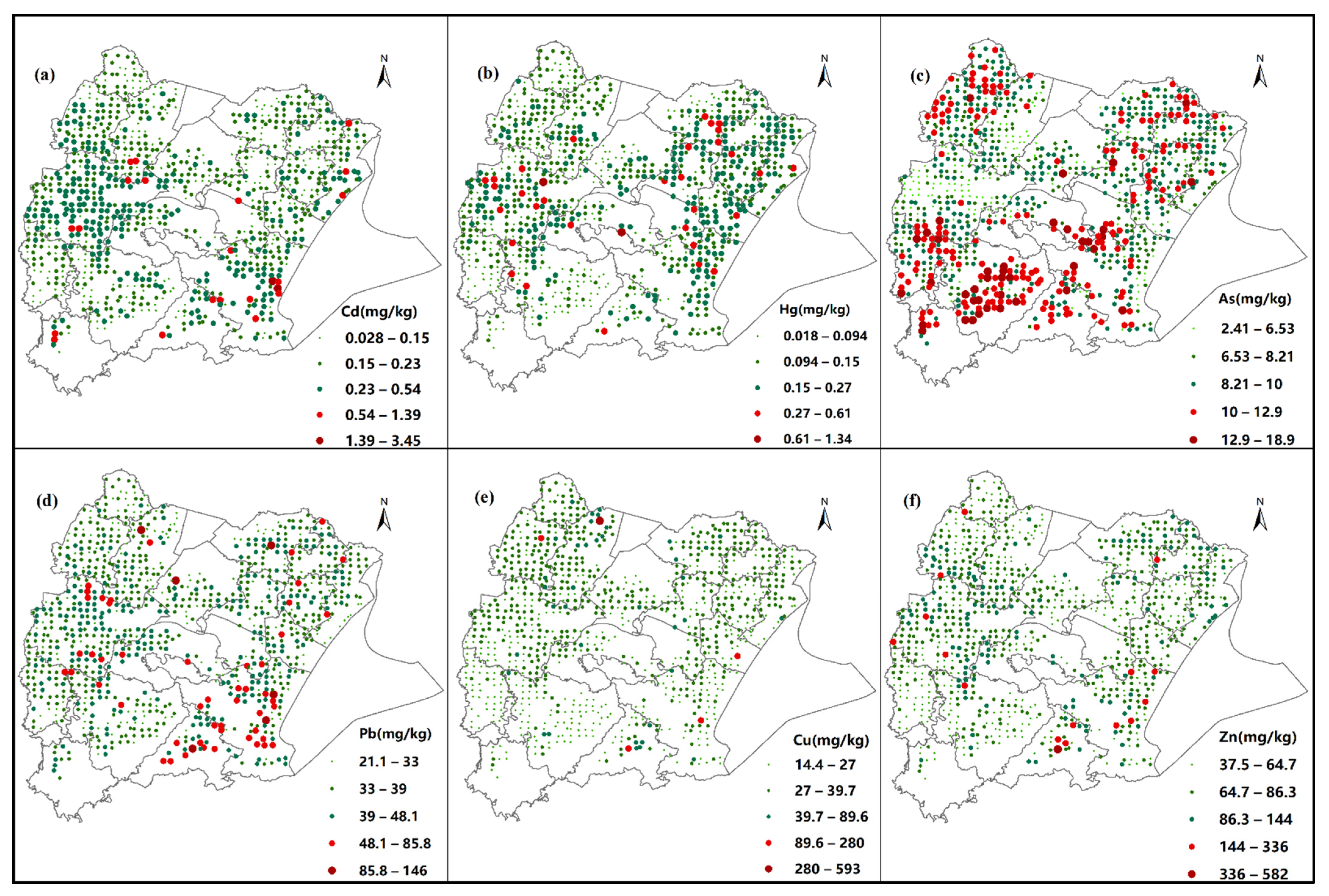
Figure 3.
Comparison of predicted value by BP model and measured values for As (a) and Hg (b).
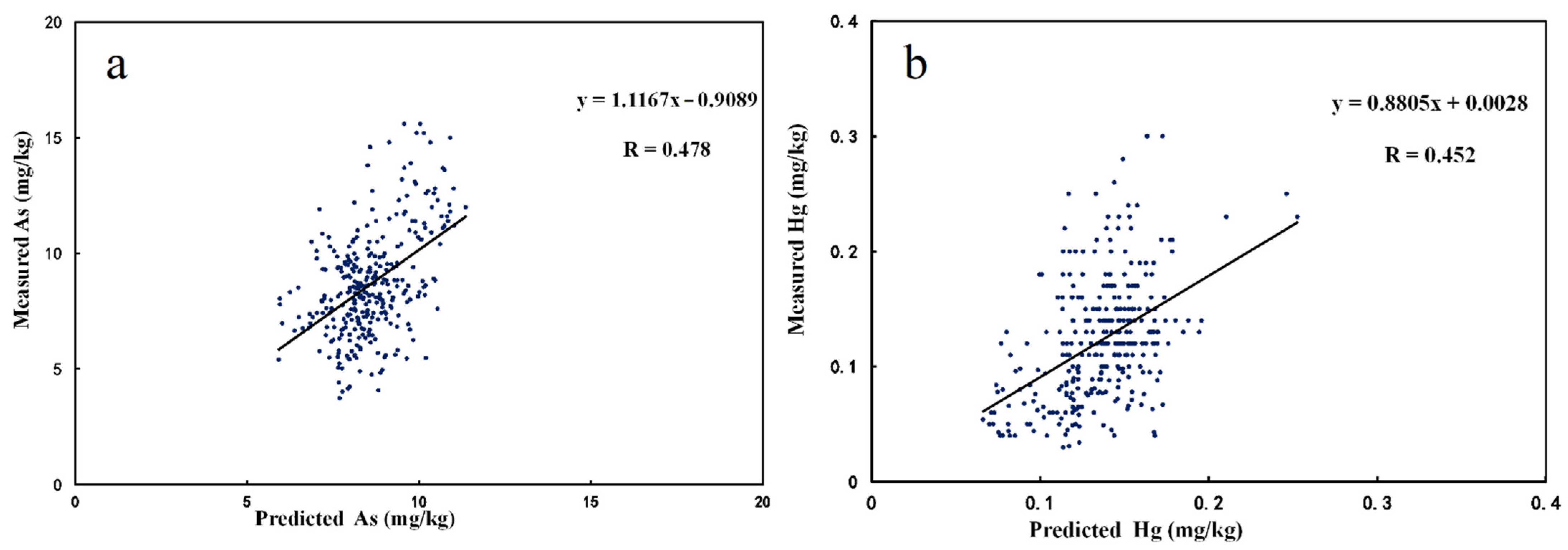
Figure 4.
Filled contour maps of As content (a,b) and Hg content (c,d) produced by ordinary Kriging interpolation and IDW interpolation.
Figure 4.
Filled contour maps of As content (a,b) and Hg content (c,d) produced by ordinary Kriging interpolation and IDW interpolation.
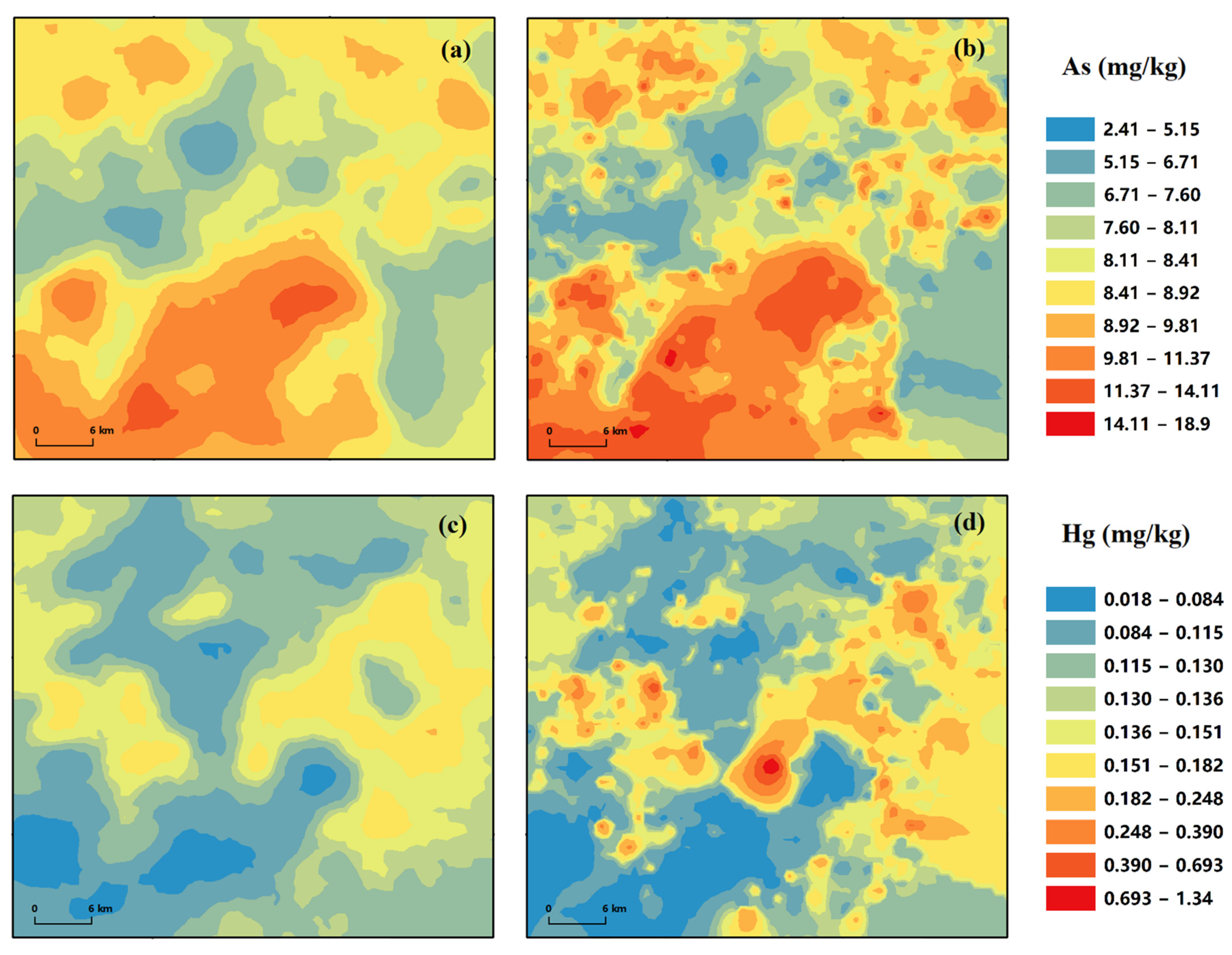
Figure 5.
Distribution map of factories in the study area.

Table 1.
A statistical contrast of the contents of six metals with national data (mg/kg).
| Element | Cd | Hg | As | Pb | Cu | Zn |
|---|---|---|---|---|---|---|
| Maximum | 3.450 | 1.340 | 18.900 | 146.000 | 593.000 | 582.000 |
| Minimum | 0.028 | 0.018 | 2.410 | 21.100 | 14.400 | 37.500 |
| Mean | 0.216 | 0.132 | 8.625 | 28.003 | 29.348 | 72.574 |
| Standard deviation | 0.177 | 0.081 | 2.249 | 9.629 | 21.800 | 27.803 |
| Coefficient of variation (%) | 81.9 | 61.3 | 26.0 | 32.1 | 74.2 | 38.3 |
| Background value | 0.13 | 0.29 | 10 | 26.2 | 22.3 | 62.6 |
| Chinese soil criteria | 0.3 | 0.5 | 40 | 80 | 150 | 200 |
Table 2.
Correlation analysis of six metals with bands.
| Cd | Hg | As | Pb | Cu | Zn | |
|---|---|---|---|---|---|---|
| B1 | 0.045 | 0.212 ** | −0.370 ** | −0.071 | 0.089 | 0.013 |
| B2 | 0.040 | 0.248 ** | −0.385 ** | −0.071 | 0.033 | 0.013 |
| B3 | 0.034 | 0.222 ** | −0.401 ** | −0.085 | 0.013 | 0.014 |
| B4 | 0.046 | 0.228 ** | −0.321 ** | −0.030 | 0.035 | 0.029 |
Note: * p < 0.05, ** p < 0.01.
Table 3.
Correlation analysis of target metals with spectrum indicators.
| B1 | B2 | B3 | B4 | B5 | B6 | B7 | B8 | B8A | |
|---|---|---|---|---|---|---|---|---|---|
| As | −0.370 ** | −0.385 ** | −0.401 ** | −0.321 ** | −0.245 ** | −0.067 | −0.035 | −0.02 | −0.003 |
| Hg | 0.212 ** | 0.248 ** | 0.222 ** | 0.228 ** | 0.156 ** | 0.057 | 0.053 | 0.057 | 0.055 |
| LnB1 | LnB2 | LnB3 | LnB4 | NDVI | |||||
| As | −0.397 ** | −0.430 ** | −0.431 ** | −0.342 ** | −0.127 ** | ||||
| Hg | 0.222 ** | 0.254 ** | 0.231 ** | 0.234 ** | 0.128 ** | ||||
Note: * p < 0.05, ** p < 0.01.
Table 4.
The results of partial least square regression (PLSR) between heavy metal concentrations and spectrum indicators.
Table 4.
The results of partial least square regression (PLSR) between heavy metal concentrations and spectrum indicators.
| Modeling Factors | Modeling Set | Verification Set | |||
|---|---|---|---|---|---|
| R | RMSE | R | RMSE | ||
| As | B1–B4 | 0.431 | 1.976 | 0.502 | 2.045 |
| B1–B4 & NDVI | 0.432 | 1.976 | 0.498 | 2.048 | |
| LnB1–LnB4 | 0.460 | 1.945 | 0.524 | 2.009 | |
| LnB1–LnB4 & NDVI | 0.462 | 1.943 | 0.526 | 2.007 | |
| B1–B4 & LnB1–LnB4 | 0.446 | 1.961 | 0.536 | 1.999 | |
| Hg | B1–B4 | 0.257 | 0.062 | 0.155 | 0.105 |
| B1–B4 & NDVI | 0.263 | 0.062 | 0.149 | 0.125 | |
| LnB1–LnB4 | 0.259 | 0.062 | 0.155 | 0.191 | |
| LnB1–LnB4 & NDVI | 0.268 | 0.066 | 0.161 | 0.105 | |
| B1–B4 &LnB1–LnB4 | 0.260 | 0.062 | 0.152 | 0.105 | |
Table 5.
The results of back propagation neural network (BPNN) between heavy metal concentrations and spectrum indicators.
Table 5.
The results of back propagation neural network (BPNN) between heavy metal concentrations and spectrum indicators.
| Modeling Factors | Modeling Set | Verification Set | |||
|---|---|---|---|---|---|
| R | RMSE | R | RMSE | ||
| As | B1–B4 | 0.530 | 1.860 | 0.507 | 2.048 |
| B1–B4 & NDVI | 0.513 | 1.865 | 0.532 | 1.999 | |
| LnB1–LnB4 | 0.519 | 1.874 | 0.467 | 2.097 | |
| LnB1–LnB4 & NDVI | 0.482 | 1.870 | 0.499 | 2.054 | |
| B1–B4 & LnB1–LnB4 | 0.497 | 1.909 | 0.525 | 2.006 | |
| Hg | B1–B4 | 0.273 | 0.062 | 0.149 | 0.105 |
| B1–B4 & NDVI | 0.318 | 0.062 | 0.177 | 0.105 | |
| LnB1–LnB4 | 0.263 | 0.061 | 0.163 | 0.105 | |
| LnB1–LnB4 & NDVI | 0.269 | 0.062 | 0.156 | 0.288 | |
| B1–B4 & LnB1–LnB4 | 0.292 | 0.061 | 0.186 | 0.105 | |
Publisher’s Note: MDPI stays neutral with regard to jurisdictional claims in published maps and institutional affiliations. |
© 2021 by the authors. Licensee MDPI, Basel, Switzerland. This article is an open access article distributed under the terms and conditions of the Creative Commons Attribution (CC BY) license (https://creativecommons.org/licenses/by/4.0/).
Share and Cite
MDPI and ACS Style
Zhao, H.; Liu, P.; Qiao, B.; Wu, K. The Spatial Distribution and Prediction of Soil Heavy Metals Based on Measured Samples and Multi-Spectral Images in Tai Lake of China. Land 2021, 10, 1227. https://doi.org/10.3390/land10111227
AMA Style
Zhao H, Liu P, Qiao B, Wu K. The Spatial Distribution and Prediction of Soil Heavy Metals Based on Measured Samples and Multi-Spectral Images in Tai Lake of China. Land. 2021; 10(11):1227. https://doi.org/10.3390/land10111227
Chicago/Turabian StyleZhao, Huihui, Peijia Liu, Baojin Qiao, and Kening Wu. 2021. "The Spatial Distribution and Prediction of Soil Heavy Metals Based on Measured Samples and Multi-Spectral Images in Tai Lake of China" Land 10, no. 11: 1227. https://doi.org/10.3390/land10111227
Note that from the first issue of 2016, this journal uses article numbers instead of page numbers. See further details here.