
Spatial Estimates of Soil Moisture for Understanding Ecological Potential and Risk: A Case Study for Arid and Semi-Arid Ecosystems

U.S. Geological Survey, Fort Collins Science Center, 2150 Centre Ave, Bldg. C, Fort Collins, CO 80526, USA
*
Author to whom correspondence should be addressed.
Land 2022, 11(10), 1856; https://doi.org/10.3390/land11101856
Submission received: 10 June 2022
/
Revised: 25 August 2022
/
Accepted: 3 September 2022
/
Published: 20 October 2022
(This article belongs to the Section Soil-Sediment-Water Systems)
Abstract
:Soil temperature and moisture (soil-climate) affect plant growth and microbial metabolism, providing a mechanistic link between climate and growing conditions. However, spatially explicit soil-climate estimates that can inform management and research are lacking. We developed a framework to estimate spatiotemporal-varying soil moisture (monthly, annual, and seasonal) and temperature-moisture regimes as gridded surfaces by enhancing the Newhall simulation model. Importantly, our approach allows for the substitution of data and parameters, such as climate, snowmelt, soil properties, alternative potential evapotranspiration equations and air-soil temperature offsets. We applied the model across the western United States using monthly climate averages (1981–2010). The resulting data are intended to help improve conservation and habitat management, including but not limited to increasing the understanding of vegetation patterns (restoration effectiveness), the spread of invasive species and wildfire risk. The demonstrated modeled results had significant correlations with vegetation patterns—for example, soil moisture variables predicted sagebrush (R2 = 0.51), annual herbaceous plant cover (R2 = 0.687), exposed soil (R2 = 0.656) and fire occurrence (R2 = 0.343). Using our framework, we have the flexibility to assess dynamic climate conditions (historical, contemporary or projected) that could improve the knowledge of changing spatiotemporal biotic patterns and be applied to other geographic regions.
1. Introduction
Soil temperature and moisture (hereafter, soil-climate) influence plant physiological function and are important determinants of plant growth and regeneration. Knowledge of soil-climate conditions, especially with the spatiotemporal context, improves the understanding of climate-ecosystem connections, including drought effects, crop yields, rangeland and forest productivity, wildfire risks, landslide potential, flood risks, dust storm potential, responses to climate change, habitat restoration and recovery and wildlife habitat selection [1]. For example, increased fire frequency and extent were linked to climate trends via elevated temperatures, the duration of droughts and snowmelt timing [2,3,4,5]. Soil moisture, in particular, is a limiting factor in arid and semi-arid ecosystems [6], with implications for primary productivity, diversity and ecological integrity [7,8]. However, a lack of mapped soil-climate data has limited research and management efficacy, especially for arid and semi-arid ecosystems within the western United States.
Many methods have been used to measure, estimate and map soil moisture. Primarily, these have included measurements at facilities [9], creating a sparse distribution of expensive point measurements to maintain and collect [10]; long-term data are also generally lacking. Recent methods include remotely sensed soil moisture mapping, which relies on microwave, synthetic aperture radar or optical and thermal infrared sensors. The remote sensing of soil moisture provides estimates at depths of ~1 mm for optical and at 5 cm for microwave [11,12,13] or deeper (5–10 cm), depending on the vegetation cover [1]. Many satellites developed for mapping soil moisture have a spatial resolution of 11–40 km [13,14,15], but less direct methods for estimating soil moisture from vegetation characteristics using visible and near infrared spectra can include ≥30 m resolution, e.g., [16,17]. The temporal resolution for satellites used for these purposes occurs between 1 and 3 days, but sub-kilometer products have >12 days, e.g., [14,15,18,19]. The spectral wavelengths used with less direct methods to estimate soil moisture have older launch dates (e.g., 1970s) [16], but sensors specific to mapping soil moisture relying on longer wavelengths (e.g., C- and X-bands) have more recent launches (e.g., ~2000s) [15,18]. The remote sensing of soil moisture is useful for near real-time applications that can capture short-term variance at the surface, such as the estimation of crop yields or assessments of herbaceous plants (e.g., fuel loading). They are less helpful in understanding ecological processes affected by soil moisture stored at deeper depths and for longer periods. However, hybrid approaches that combine remotely sensed estimates and models support a much larger suite of applications [20,21,22], including uses for crops [23], hydrologic models [24] and near real-time estimates at greater depths [1,14,15,18].
Models of soil moisture estimates can support analyses of historical, contemporary and projected climates of multiple spatiotemporal scales, allowing for an increased understanding of soil-climate variability and biological processes. A few models include SOILWAT [25,26], SoilClim [27], Hydrus 1-3D [28,29,30,31], soil-water-atmosphere-plant (SWAP) [32] and soil-water-balance (SWB) [33]. Modeling soil moisture requires estimates of potential evapotranspiration (PET or ETo), for which there are more than 50 methods [34], soil properties, climate/weather data and factors affecting radiation forcing [35]. We highlight two common models using different ETo models. The SoilClim model [27] uses Penman–Monteith to estimate ETo [36] and accounts for snow accumulation and melt to estimate soil moisture and snow water balance, similarly to spatial_nsm. However, the Penman–Monteith estimation of ETo requires a suite of atmospheric data with limited availability (e.g., not spatially continuous or available in atmosphere-ocean general circulation model [AOGCM] projections). Specific to dominant vegetation across the semi-arid sagebrush biome, a couple studies used the SOILWAT model [37,38,39], including a seasonal soil moisture pattern for sagebrush ecosystems that relate spring recharge followed by extended drying.
Soil–climate interactions with below- and above-ground physical and biological processes occur at varying temporal and spatial scales. Soil temperature affects biological, chemical and physical processes [40], and it is affected by thermal conductivity and heat capacity, which are regulated by solar radiation, the latent heat of condensation and evaporation [41]. In particular, soil respiration and decomposition (i.e., carbon budgets) are positively connected to soil moisture and temperature [42,43,44]. Soil temperature varies among differing topographies [45,46], vegetation covers [46,47,48] and snow covers [49,50,51,52]. Soil temperature fluctuates by depth and time of day due to the variation of radiation, heat exchange at the air–soil boundary and heat transfer within soils due to thermal properties [53,54]. The conduction of heat within soils is slow, where shallow soils can have increased temperature anomalies due to diurnal variations in radiation, and deep soils are affected by long-term average temperatures with less temporal fluctuation [40,53].
Atmospheric conditions influence the amount of water supplied to the soil and its removal rate (controlled by temperature, radiation, humidity and wind speed). The gravitational drainage of soils occurs on a timescale of ~1 day, but studies show that these processes can occur on a scale of months, where the variability is greatest for shallower depths (e.g., cm) and is smallest at greater depths (e.g., meters) [55]. Groundwater is also an important factor affecting soil moisture, but it is seldom considered. For example, a shallow groundwater table reduces the vertical downward movement of soil water, which increases soil moisture [35]. At small spatial scales (e.g., catchment), hydrologic conductivity, vegetation types, soil types and soil porosity affect soil moisture [56,57,58]. Precipitation and radiative factors primarily affect soil moisture at large scales [55,59]. Fine-scale patterns of topography, soil physical properties and vegetation cover influence the effects of incoming solar radiation and therefore soil-climate, especially in dry environments [1,14,15,18]. Additional interactions within the soil-plant-atmosphere continuum, such as changes in stomatal behavior with changes in CO2 and the access to non-surface water by roots, can influence soil moisture estimates [60,61], but the importance of drought monitoring to help forecast and mitigate climate change effects outweighs the challenges encapsulated by different measurement and modeling approaches.
The effects of snow on soil-climate are not fully understood due to snow’s spatial heterogeneity, depth, persistence and physical structure, which demonstrate considerable temporal variability [62]. However, changes in snowpack are known to affect soil moisture (the amount and timing of water input) and temperature (insulation), with ensuing effects on ecosystem functions and plant composition. Snow is the dominant precipitation input for sagebrush steppe occurring in the western United States [63], where soils are typically cool and moist during the early growing season, warm and dry during the mid-to-late growing season and partially frozen during winter [64,65]. For example, altered snowmelt timing can increase the fecundity and survival of cheatgrass (Bromus tectorum L.) [66], an invasive species significantly affecting the western United States. Research also demonstrates that the thermal insulating effect of snow is greatest with deep snow (>80 cm) [67], causing winter soil temperatures to be ~1–2 °C warmer with shallow snow (≤40 cm) and 4 °C warmer with deeper snow [68]. With the anticipated temperature changes from climate change, snowpack reductions are expected to be most impactful for mid-to-high-elevation ecosystems, altering soil respiration and affecting soil carbon storage, efflux and nutrient cycling [67].
Understanding the distribution, growth and recovery of vegetation in arid and semi-arid environments is crucial for rangeland managers. Plants of these systems thrive through physiological adaptations that support a range of conditions resulting in irregular distributions. For example, the distribution of big sagebrush subspecies (Artemisia tridentata ssp. Nutt.), a keystone species in the ubiquitous semi-arid shrublands of the western United States, vary in response to drought [69] and temperature [70,71,72], with mechanisms tied to germination and seasonal phenology [73]. The growth and photosynthesis of sagebrush are greatest near 20 °C [70,74]; however, warmer temperatures during spring and summer may hinder growth in warm-dry habitats [75,76] and improve growing conditions in colder climates [77,78,79]. In rangelands of the Colorado Plateau (southwestern United States), plant productivity was reduced with decreasing soil moisture—regardless of temperature [80]. Temporal scales and the cycling of processes in arid and semi-arid environments are also important for rangeland managers. For example, productivity patterns in shrublands were correlated with 6–12 month drought indices, and grasslands were correlated with 3–6 month drought indices [80], confirming the differentiation of vegetation due to soil moisture and monthly scales. Such patterns indicate how the vegetation of semi-arid environments is adapted to specific, limiting and variable conditions, making conservation and management prescriptions challenging.
Habitat conservation and management in semi-arid landscapes are challenging due to the limiting environmental conditions, especially soil moisture. The lack of mapped soil-climate data can limit research and management because of unexplained spatial and temporal heterogeneity; soil texture, climate normals and elevation are typical surrogates [81]. Multiple-use management that sustains the habitat for wildlife and domestic livestock in this semi-arid environment is challenging due to the variability in limiting conditions that leads to unexplained and undesired outcomes, such as seedling mortality. Thus, this work aimed to improve the understanding of fundamental ecosystem properties through a soil-climate model with high spatial and temporal resolution data inputs directly affecting ecosystem conditions.
We developed a new implementation of the Newhall soil simulation model (NSM) [82,83,84,85] to map estimates of soil-climate conditions (e.g., soil moisture and temperature characteristics). Our objectives included the following: (1) develop a spatially explicit implementation of the NSM that supports spatial data inputs and outputs at spatial resolutions sufficient to inform local management, (2) create a soil-climate model that can support different climate conditions, (3) support different PET methods, (4) account for snow (e.g., snowmelt, attenuation of evaporation and insulation of soil), (5) account for air-soil temperature offsets, (6) estimate soil moisture and (7) reliably produce soil temperature-moisture classifications. These objectives address recognized limitations and improve the product availability for researchers and managers. For this study, we used climate normals (1981–2010) to produce gridded surfaces (spatial resolution of 30 m) of soil moisture (monthly, annual and seasonal), soil temperature and moisture regimes (STMR), seasonal moisture trends and seasonality indices (hereafter, soil-climate products). To evaluate the utility of our soil-climate products for sagebrush ecosystem management, we investigated the explanatory power between modeled soil-climate results and ecosystem conditions (e.g., sagebrush cover, exposed bare ground, annual herbaceous plant cover and fire frequency). Although our example was specific to the sagebrush biome and climate averages, these methods may be applied to other geographic regions with different temporal resolutions of climate data and user-specified parameters.
2. Methods and Materials
2.1. Study Area
Our study area encompasses the sagebrush biome in western North America, which occurs east of the Sierra Nevada and Cascade Mountain ranges and west of the Great Plains in the United States (Figure 1). This region is geographically, geologically and hydrologically diverse, including major physiographic regions of the Rocky Mountains, Intermontane Plateaus and Pacific Mountains [86,87]. The sagebrush biome typically has hot, dry summers and cool-to-cold, moist winters (Table 1). Vegetation communities vary with precipitation, temperature, soils, topographic position and elevation [88].
The basins and plateaus in this region are dominated by sagebrush (Artemisia spp.) shrublands and steppe with conifer, aspen and mixed forests and woodlands at higher elevations, salt deserts at the lowest elevations and a mixture of shrub and grasslands in the western Great Plains [90,91] (chapter A). Big sagebrush species (A. tridentata Nutt.) generally occur on well-drained, moderately deep and sandy-to-clay-loam soils, while low sagebrush species predominately occur on shallow or poorly drained soils due to a shallow duripan or bedrock (30–50 cm) [88]. The sagebrush biome supports important wildlife, including many ungulate and avian sagebrush-associated species, which have been affected by the increasing prevalence of non-native annual grasses (e.g., Bromus tectorum L. and Taeniatherum caput-medusae (L.) Nevski), wildfires, habitat degradation due to land-use, conifer expansion and extended droughts and weather variability [91] (chapters J-P).
The U.S. Bureau of Land Management (BLM) is responsible for managing 78.4 million hectares of sagebrush habitats, where greater sage-grouse (Centrocercus urophasianus) inhabit 150 million acres. Greater sage-grouse are an important sagebrush-obligate species that are considered a conservation umbrella [91], where populations have experienced 80% declines in abundance since 1965 [92]. The sage-grouse range includes some of the best remaining intact sagebrush (Figure 1). Importantly, BLM managers identified the amount and timing of precipitation, seasonality (variation among seasons) and soil moisture as important data for management success [93]. Seasonal soil conditions were considered important for seeding and fuels management, while snow was recognized for its effect on spring and winter soil moisture [93].
2.2. Modeling Overview
Developing a spatially explicit soil-climate model involved several steps (Figure 2): (1) identifying and processing spatial input data, (2) processing and collecting data to enhance the model, (3) executing models on a high-performance cluster and (4) identifying key post-analysis products and evaluating soil-climate estimates. For step one, we acquired spatial data representing monthly precipitation and temperature [94], daily snow deposition [95], soil physical properties (Polaris) [96,97], monthly averages from climate stations [89,98] and daily soil conditions from the soil climate analysis network (SCAN) [99]. Descriptions of the data sources are provided in the (Supplemental Materials S1; Table S1), and their uses are explained below. For step two, we used additional data to enhance our model, including the SCAN database to define monthly ambient-temperature offsets, snow cover to account for the attenuation of PET and offset soil temperature and organic matter to inform the classification of temperature regimes. Steps three and four are outlined in Section 2.6 and Section 2.9, respectively. For our analyses, we developed and used an open-source software (spatial_nsm; Supplemental S2) relying on PythonTM that was translated from jNSM software (v. 1.6.1) [100]. We used Esri© ArcProTM [101] to compare independent data and Program R [102] for statistical analyses. Most of the modeling and analyses depended on a high-performance computing cluster (see Supplemental S3) [103].
2.3. Precipitation
We used climate averages (30-year normals: 1981–2010) defined by the parameter elevation regression on independent slopes model (PRISM), representing monthly temperature and precipitation estimates on continuous gridded surfaces [94]. These data provide precipitation and temperature based on climate station observations and weighted regression that account for climate regions, orographic effects, topographic orientation, rain shadows, temperature inversions and coastal proximity [104]. The PRISM precipitation reflects water as solid (i.e., snow) and liquid (i.e., rain) for each month. Because solid precipitation cannot infiltrate soil, we used solid and liquid precipitation modeled from the snow data assimilation system (SNODAS) [95] to determine liquid–solid ratios. We then calculated an adjusted precipitation (monthly liquid precipitation as rain and snowmelt) as a model input with these ratios.
The SNODAS estimates daily snow properties (e.g., snow cover/redistribution, liquid precipitation, depth, melt and sublimation) from a remote sensing platform (moderate resolution imaging spectroradiometer; MODIS), snow telemetry stations (SNOTEL) and a model to provide data on snowpack properties. We calculated monthly averages (normals) from daily SNODAS data, including solid precipitation (product identifier: 1025SlL01; data scale factor = 10), liquid precipitation (1025SlL00; scale = 10), snowmelt (1044; scale = 100,000) and snow depth (1036; scale = 1000). The scaled data for solid and liquid precipitation, snowmelt and snow depth were converted to kg/m2, kg/m2, mm and mm, respectively, and no data pixels were assigned zero. We defined normals for all of the SNODAS daily estimates (Equation (1)) and calculated monthly normal liquid ratios to estimate monthly precipitation falling as liquid (Equation (2)). Using the monthly normal liquid ratios, PRISM precipitation and SNODAS snowmelt, we computed an adjusted precipitation (monthly liquid precipitation as rain and snowmelt; Equation (3)). These equations yielded monthly liquid precipitation (i.e., rain and snowmelt) relative to PRISM precipitation amounts.
where SNODASi reflected monthly normal conditions, i represented the SNODAS product, dSNODAS was the daily product, s reflected a unit conversion applied to the source data (scale) and monthst was the number of occurrences per month across all years.
where liqm_ratio denoted the SNODAS liquid ratio for monthly normals, SNODASliq denoted the monthly normal liquid product and SNODASsol denoted the monthly normal solid product. (Equation (1)).
where pptm_adj denoted the monthly normal adjusted precipitation denoting the amount of water that can infiltrate the soil, liqm_ratio denoted the SNODAS liquid ratio for monthly normals, PRISMm_ppt denoted the monthly normal precipitation, snowmeltm and snowmelta denoted the SNODAS snowmelt monthly and annual normals, respectively, and PRISMa_ppt denoted the precipitation annual normal.
2.4. Temperature
Microtopography influences localized temperature and therefore soil moisture. Such characteristics are important for describing the success of shrub-steppe seedbanks [105], shrub distribution and diversity [106,107,108] and for understanding the spatial configuration and distribution of terrestrial vegetation communities [109], such as forests [110] and alpine plants [111]. We accounted for microtopography in soil-climate estimates by statistically downscaling temperature [112]. We downscaled the PRISM monthly mean temperature (800 m), where the explanatory variables reflected PRISM monthly mean temperature normals (1981–2010) and terrain indices describing microtopography. The response variable represented the climate station monthly normal (1981–2010) [89,98,113] at 1507 stations (Supplemental S4, Figure S3A). The primary terrain components included a hydrologically corrected digital elevation model (DEM), vector ruggedness measure (VRM) [114] and heat load index (HLI) for mid-latitudes [115,116], where the coolest slopes occur on northeast aspects and the warmest slopes occur on southwestern aspects (data description in Supplemental S1).
Before deciding on a downscaling approach, we explored the explanatory power of the covariates and the spatial autocorrelation for all candidate covariates. We determined that no significant spatial autocorrelation existed using spatial regression models (the lag and error model). We then used random forest machine learning (Python library scikit-learn and RandomForestRegressor function) [117] to define downscaled 30 m monthly mean temperature surfaces (30-year normal). The labels used in the random forest represented our response variable, and the features (explanatory variables) reflected the candidate covariates. We assessed 200 and 1000 trees, but selecting 200 as additional trees did not improve the model, and we withheld 20% of climate stations to evaluate the model performance (cross-validation). The model with the best overall fit (based on R2, performance measures and cross-validation results) across months was selected (see Supplemental S5) [118,119]. We expected the downscaling of temperature to have less of an influence during the winter months because of a lower sun angle and the potential presence of snow cover.
2.5. Available Water Capacity
The available water capacity (AWC; field capacity—permanent wilting point) is the water held in soil between the field capacity (nearly saturated, −33 kPa) and the permanent wilting point (extremely dry, −1500 kPa), representing the potential capacity of the soil to retain water based on its properties [120]. We calculated the AWC using Polaris soil properties [96] at six incremental depths to 200 cm and the van Genuchten method [121]. We accomplished this by estimating the field capacity and wiling point using the van Genuchten method (Supplemental S6; Equation (1)) [121]. The thetar (wilting point) and thetas (field capacity) provided with Polaris data are estimated with the pedotransfer function NeuroTheta, which relates observed soil properties to hydraulic properties [96]. The potential soil water content is then calculated for the two pressures relating to saturated (−33 kPa) and residual/wilting (−1500 kPa) conditions, which provides the information to calculate AWC (see Supplemental S6 for equations). With AWC values calculated at each incremental depth and pixel, we derived a summed value following Lytle, et al. [122], resulting in a single AWC value for the 0–200 cm soil profile. Therefore, the soil properties define the capacity to retain water (i.e., available water capacity), which informs how the Newhall simulation estimates the accretion and depletion of water within the soil profile based on the energy (PET) available for extracting moisture.
2.6. Newhall Simulation Model
The NSM is an accounting system of water movement in a vertical soil profile and characterizes the soil moisture and soil temperature conditions [82,83,84,85] using monthly precipitation (total), monthly air temperature (mean) and AWC as data inputs. The model uses the Thornthwaite–Mather–Sellers PET equation [123,124,125] to reflect the energy available for extracting moisture (Supplemental S7), but other methods can be exchanged within spatial_nsm. This daily, enumerated simulation of soil moisture movement is based on a two-dimensional diagram of the soil profile (Supplemental S8) [83]. The profile extends from the ground surface to a depth characterized by AWC estimates—in our case, 200 cm. For example, clay materials can support an AWC of 200 mm with a soil depth of 80 cm, while sandy loam with an AWC of 200 mm might be as deep as 200 cm [83,126]. The STMR classifications described by the Natural Resources Conservation Service (NRCS) in Soil Taxonomy [120] and Keys to Soil Taxonomy [127] were the foundation for classifying soil-climate regimes; however, we implemented a revised dichotomous approach based on Paetzold [128] to correct null classifications occurring with previous approaches. Classifications of STMRs are produced for the soil moisture control section (SMCS; ~50 cm), and soil moisture—uniquely extracted with our software—reflects the depth AWC computed (0–200 cm). We made several additional adjustments to the data inputs, model parameters and spatial predictions to reduce NSM limitations (Table 2, Section 2.7). Notably, we created a spatial implementation of the NSM using the following data: (1) monthly, downscaled temperature (mean); (2) monthly, adjusted precipitation (total); and (3) AWC calculated from Polaris data. Our software (spatial_nsm) also supported additional data to improve soil moisture estimates, including organic matter, snow depth and monthly air-soil temperature offsets (see Section 2.7).
2.7. Custom Model Parameters
We used three methods to improve the estimates of soil temperature at 50 cm within spatial_nsm. These included using monthly air-soil temperature offsets, accounting for the insulation of soils due to snow cover and using an organic horizon when classifying the soil temperature regime. The Newhall simulation model assigns soil temperature at an average 50 cm depth based on air temperature and an air-soil offset. Previous research uses a default air-soil temperature offset where the soil temperature is 2.5 °C cooler than the air temperature due to the lack of spatially explicit data [132,133]. We used hourly data collected from soil temperature sensors of the SCAN database [99] to improve the estimation of this offset for climate averages. We calculated normal monthly mean soil temperature at 50 cm using SCAN observations between 1988 and 2020. The SCAN network included 61 stations within our study area (Supplemental Figure S3B), for which we calculated a monthly mean across all available years to define our monthly air-soil temperature offsets as an alternative to using a single offset value of 2.5 °C (Supplemental S4, Figure S4, Table S2).
Snow cover insulates soils and results in warmer soil temperatures relative to the ambient temperature [136,137], but few studies provide detailed information on how differing snow depths affect soil temperature (see Supplemental S4). Smith, Newhall, Robinson and Swanson [40] described the results of a study [138] where soil temperature and air temperature on bare and snow-covered sites at Leningrad, Russia (now Saint Petersburg) were observed. Inferred from these results, we approximated estimates of monthly soil temperature offsets for snow-covered ground. We used SNODAS snow depth (Equation (1)) and calculated the proportion of days within a month (normals), where snow was ≥12 cm in depth. Because we were working with monthly normals, we adjusted soil temperature when >50% of days had ≥12 cm of snow cover for a given month as a conservative estimate (Supplemental S4, Table S3).
The soil taxonomy handbook [120] differentiates between cryic and frigid soil-temperature regimes (see Supplemental S9) when organic matter ≥ 20%; however, this criterion is not considered in any software assigning soil-climate classifications. An organic horizon is defined as a soil layer that is saturated with water for longer than 30 days (cumulative) per year in normal years and contains ≥ 20% organic carbon [120]. Organic matter increases moisture retention, and a higher moisture content results in a longer heat retention due to the heat capacity of water [139]. We used Polaris organic matter by depth (log10 [%] scaled data) to account for soil insulation. We converted the scaled data (0–5 cm depth median product) to percent organic matter by raising the pixel values to the power of ten. Any pixel with organic matter ≥ 20% was used to differentiate between cryic and frigid soil-temperature regimes (see Supplemental S9) based on the soil taxonomy STMR definitions [120]. Supplemental S9 and S10 provide details on the STMR keys used in spatial_nsm based on Paetzold [128].
Lastly, we used SNODAS snow depth (Equation (1)) to account for the reduction of evaporation that could result from soils covered with snow [140,141]. With spatial_nsm, we adjusted PET by accounting for the proportion of days with sufficient snow (≥12 cm of snow cover) that attenuated evapotranspiration (Equation (4)).
where PETm_adj is the monthly adjusted potential evapotranspiration PET due to snow cover, snowdays_ratio is the ratio of days within a normal month with snow cover ≥12 cm and PETraw is the Thornthwaite–Mather–Sellers calculation used within the Newhall simulation model.
2.8. Soil-Climate Post-Analysis
Using monthly soil moisture estimates, we generated Theil–Sen estimates (90% confidence interval [CI]) [142,143] for March to September (entire growing season) and March to June (early growing season). The Theil–Sen method estimates a median of slopes and intercepts from all pair-wise combinations—in this case, the successive monthly estimates at each cell location—and provides a robust trend estimate. These results supported the visual and statistical interpretation of spatial patterns in soil moisture trends, aiding the investigation of vegetation growth and fuel conditions. We also calculated seasonality for two periods (standard deviation), including spring (March, April, May and June in the Northern Hemisphere or September, October, November and December in the Southern Hemisphere) and seasonal conditions (spring, summer, fall and winter). Descriptive attributes of the dominant vegetation associated with soil-climate regimes (STMR) were determined by using spatial correlation to quantify the distribution of Landfire existing vegetation types (EVT) within STMRs [144]. The EVT attributes were summarized by STMR (ArcGIS Pro; geoprocessing tool Zonal Statistics as Table) [101] to identify plant community associations (e.g., big sagebrush steppe and shrubland, montane sagebrush steppe, low sage steppe, montane oak and mixed shrubs and aspen forest and woodland) with ecologically similar soil temperature and moisture regimes. The derived products were used to investigate the relationships between the vegetation (types and cover) and soil-climate to describe dominant vegetation associations.
2.9. Evaluation
We used three approaches to evaluate our results by comparing them to other products. First, we investigated the standardized international soil moisture network (ISMN) database [9,145,146] within our study area (~2.4 million km2) as an independent source of in situ sensors to evaluate the performance of soil moisture estimates (Section 3.3). Using the ISMN data, we removed poor-quality data (defined by ISMN), and retained data measured at a 0.5 m depth (50 cm; closest depth comparable to our 200 cm depth), occurring between 1981 and 2010 and with >5 years of records. We identified 175 stations associated with SCAN [147] and snow telemetry networks (SNOTEL) [148]. Due to locational errors that we identified for in situ sites (ISMN data) relative to data downloaded from NRCS (min = 0; max = 26,731; mean = 594 m; errors visually verified with 1 m spatial resolution aerial photography), we corrected locations before using them. We compared the soil moisture estimates of in situ sensors to those of our 0–200 cm estimates. We also used the aspatial module of spatial_nsm to compare soil moisture estimates of in situ sensors to Polaris (30–60 cm) AWC depth; this allowed for a closer approximation of depth to in situ sites, but the aspatial code does not include the effects of snow handled in the spatial module of spatial_nsm. Statistical tests for the evaluation included Pearson’s r and unbiased root-mean-square error (ubrmse) [149]. Second, we evaluated 1280 climate stations and compared our results from a spatial_nsm to the results from jNSM v. 1.6.1 [100] using identical and differing data inputs and parameters (see Supplemental S11 for methods; Section 3.4). Third, we compared STMR results to NRCS classifications (gNATSGO) [134] and a second classification derived from NRCS data used to inform resistance and resilience concepts (Section 3.5) [131,150,151].
Because a purpose of the spatial_nsm results was to inform habitat research and management, we assessed the statistical relationships between the ecosystem components of sagebrush cover, bare ground, annual plants (predominantly invasive species), wildfires (frequency) and soil-climate products as an indirect method of determining how our soil-climate variables aligned with biological relationships and patterns (Section 3.6). Understanding the abundance and productivity of sagebrush is important for assessing the overall rangeland health and ecological potential (recovery after disturbance), as previous research has established soil-climate as an important driver [131,150,152]. The distribution and abundance of unvegetated ground are inversely related to the total vegetation cover, providing a robust measure of habitat structure; however, causes of patterns and trends in unvegetated soil may be diverse (e.g., due to natural and anthropogenic causes) [153], so careful interpretation is warranted. Because of the considerable management concerns [154] and modeling challenges of annual herbaceous plants within our study area (for example, Bradley et al. [155] reported variance ranging from 34% for continuous cover to 77% for a classification), we assessed the explanatory power of soil-climate for these species [156]. Encouraged by the correlations between soil moisture and wildfire characteristics (size and abundance) [157,158], we assessed connections between our soil moisture and wildfire occurrence.
We applied the following statistical analyses to assess the explanatory power of soil-climate for selected vegetation and ecosystem patterns. First, we used statistical models to assess the explanatory value of STMRs and seasonal soil moisture estimates (i.e., predictors) using variance explained in the landscape distribution of sagebrush cover and bare ground [159], herbaceous annual plant cover (ANHB) [156] and burn frequency (1984–2016; Landsat burned area essential climate variable [BAECV]) [160]. The data representing annuals in 2010 reflected conditions at the end of our climate normal period (1981–2010). Second, we developed generalized additive model (GAM) comparisons to demonstrate the validity of soil-climate model results through their ability to describe habitat patterns and processes important for management and conservation. Our models used sagebrush cover, bare ground, annual herbaceous plant cover and fire frequency as response variables to reflect ecosystem conditions. We acquired remotely sensed and modeled burn data and summed burned pixels across all years (1984–2016; BAECV sum) and used annual or seasonal soil moisture estimates as independent variables in univariate models. Bivariate models included one season and a moisture trend estimate (Theil–Sen slope). Lastly, we used GAMs and compared the explanatory power of soil-climate predictors versus climate predictors to ascertain whether soil-climate was an improvement on climate data. For this evaluation (Section 3.7), we used identically structured GAMs predicting sagebrush, annual herbaceous and exposed bare ground, with independent variables of climate factors (1981–2010 normals: total precipitation and mean, maximum and minimum temperatures).
Non-linear generalized additive models in Program R (library mgcv) [161,162] were used to describe the relations between soil variables and ecosystem patterns. Each GAM model was fit using Gaussian distributions (scale = −1, gamma = 1.4) and a smoothing variable derived from geographic locations. The smoothing variable is a tensor product (te) fit using X-Y coordinates (meters), a residual maximum likelihood (REML) estimation using a Pearson estimate of the scale and a thin-plate regression spline; the base dimension (k) was set to 45 after testing by incrementally increasing k and comparing changes in the model fit and computing time [161]. The same smoothing function structure was used for all models. Parsimonious results were identified using Akaike information criteria weights (AICwi) [163]. The generalized cross-validation (GCV) score selects the smoothness parameter that minimizes prediction errors, where smaller values indicate better-fitting models [164]. To sample multiple spatial datasets, we used ArcGIS Pro (extension Geostatistical Analyst™, geoprocessing tool Create Spatially Balanced Points) to allocate 500,000 spatially balanced, random sample points, where the area within each class for soil temperature and moisture classes defined the sampling probabilities. Because not all of the data used in the comparisons were perfectly aligned (e.g., non-target masking, differing extents), we subsetted the point sample to ensure matching vector lengths and an accurate comparison; all analyses included more than 200,000 sample points yielding sufficient statistical power.
3. Results
3.1. Model Input Modifications
The results from modifying precipitation and temperature demonstrated significant advantages, especially for the accounting of snowmelt. The adjusted precipitation (Equations (1)–(3)) importantly captured the water available to infiltrate soil after snowmelt. Spatially, the effect of these modifications varied and significantly changed with when, where and how much water entered the soil system. We have illustrated these differences between unadjusted and adjusted precipitation for three watersheds within our study (Figure 3). For temperature downscaling, the best model (climate stations [n = 1507] ~ [PRISM mean temperature, heat load index, elevation, vector ruggedness measure] resulted in a strong performance, as shown with the mean absolute percentage error (MAPE; 0.18–0.24), R2 (0.93–0.96) and cross-validation mean squared error (MSE; 4.81–10.84). See the Supplemental Materials S4 for explanations of the metrics, variable importance and performance of the top two best models. The effect of using monthly temperature offsets was not quantifiable, but such offsets are more realistic for temperate conditions than using a default offset of 2.5 °C (Supplemental Figure S4).
3.2. Soil-Climate Products
Spatial data products produced by spatial_nsm (Supplemental S12; Table S8) included estimates for soil moisture (monthly, seasonal and annual), trends of spring and growing season soil moisture (Theil-Sen estimates), STMRs, the seasonal Thornthwaite moisture index (TMI; precipitation minus PET) and the soil moisture seasonality (30 m rasters; Supplemental S12, Table S8). We provide figures for a few of these products, as some were used for assessing associations between soil-climate and vegetation associations. Soil moisture (mm) is a new product we derived from the NSM, which denotes the volume of water remaining in the soil profile for a 30 m by 30 m pixel after accounting for accretion and depletion (Figure 4) and, unlike TMI, accounts for soil properties (up to 2 m). The Theil–Sen estimator of soil moisture for March to June (Figure 5a) and March to September (Figure 5b) demonstrated different rates of change (mm/normal month) that can support different research and management questions. The seasonal soil moisture reflected spring, summer, fall, winter and annual. The seasonality among seasonal moisture (Figure 6a) and spring months during the growing season (Figure 6b) show important spatial and temporal variability that can help land managers relate the importance of variability to flora and fauna needs. The STMRs (Figure 7) captured by spatial_nsm were important for comparing software accuracy and exploring the explanatory power of Landfire EVT and ecosystem component correlations (results described below) and may aid in the investigation of resistance and resilience concepts.
3.3. In Situ Evaluation
The final data available for this evaluation (209 stations) consisted of start years ranging between 1996 and 2010 (median = 2003; median number of data collection years = seven), with an elevation range of ~588 m to ~3500 m (). Our spatial soil moisture estimates reflected a period of 1981–2010. The unadjusted monthly precipitations of 1981–2010 (800 m) PRISM and 1996–2010 (4 km) PRISM were highly correlated (Pearson’s r ≅ 0.9–0.97), and, therefore, differences in the climate should have minimal effects on the evaluation. Our spatial, soil moisture estimates of volumetric water content (VWC) reflected a 0–200 cm depth, and the in situ sites reflected a single depth (~0.5 m [50 cm]; see Section 4.2 for discussion). Due to mismatches of temporal and spatial scales between in situ sites and our soil moisture estimates, we demonstrated weak relationships (Table 3; Polaris [0–200 cm]), as expected. Our evaluation of in situ sites and Polaris AWC for a depth of 30–60 cm, using the aspatial module of spatial_nsm, greatly improved the performance but maintained weak relationships. These differences are likely due to not having comparable soil depth ranges relative to in situ sites and climate mismatches and the aspatial module not accounting for several data, including PET attenuation due to snow cover.
3.4. Software Evaluation
With all parameters equal between jNSM and spatial_nsm (e.g., ten iterations and no consideration of STMRs, as these classifications differ between software), the results for 100% of the climate stations matched. Using these same methods but considering the different dichotomous classification of STMRs, 90.7% of the climate stations matched. Of these mismatched results (Supplemental Table S7), 55 stations switched from cryic (jNSM) to frigid (spatial_nsm) temperature regimes; 24 stations classified by jNSM did not assign a soil moisture regime; and all stations classified by spatial_nsm assigned a soil moisture regime. When we assessed differences between spatial_nsm with 1000 iterations of the conditioning period compared to the ten used in jNSM while not considering STMRs, we had 99.1% agreement; however, when we considered STMRs, there was 90.5% agreement.
3.5. Product Comparisons
Comparing three mapped products of STMR classifications (gNATSGO, resistance and resilience and our results) of soil temperature (Supplemental S13 and Figure S7) and soil moisture (Supplemental Figure S7) illustrated similarities and differences. We determined that a statistical comparison was impractical due to the lack of mapped soil attributes and documentation describing methods of STMR classification for products. Importantly, our soil-climate products produced greater cryic soils (converted from frigid) in high plateaus of rangelands (Supplemental S13 and Figure S7), which aligns with the differences observed when we used climate stations as an evaluation. The gNATSGO, resistance and resilience products showed significant survey differences commonly observed at state boundaries, where our soil-climate results did not include these artifacts (Supplemental S13 and Figure S7). Similarities of soil moisture regimes across all three products existed, but significant differences occurred in Montana, where our soil-climate products mapped dryer soils compared to estimates assigned by the resistance and resilience classifications (gNATSGO had significant gaps in data for moisture, and, therefore, we could not make comparisons; Supplemental Figure S8).
3.6. Ecosystem Component Correlations
Soil-climate predictors generated high and very high significance in most model comparisons using univariate and bivariate combinations. The smoothing functions (tensile spline) in GAM models significantly contributed to the explanatory power. Seasonal soil moisture models revealed significant correlations with all four response variables. Spring was frequently the strongest predictor (AICwi) among seasonal univariate models, and combinations of spring moisture with fall or winter created strong bivariate seasonal models (Supplemental Table S9). Fire frequency also produced highly significant models using soil moisture predictors (Supplemental Table S10). Bivariate models generally performed better than univariate models, indicating that combinations of seasonal moistures were useful for capturing ecological complexity.
3.6.1. Sagebrush
Sagebrush exhibited a significant positive correlation with the mesic (warm) temperature regime in combination with a range of moisture conditions, and sagebrush had the strongest positive associations (coefficient estimates) with moisture regimes between dry tempudic (very wet) and typic xeric (dry)—approximately the middle of the range (Supplemental S13, Table S11). Statistical correlations and zonal statistics indicated a mean sagebrush cover of 10–14% in just five co-dominant soil-climate types: weak xeric, typic xeric (dry) and dry aridic (very dry) moisture regimes with frigid (cold) temperatures and dry and typic xeric (dry) moisture regimes with cryic (very cold) temperatures. The spring and autumn soil moisture combination (Supplemental S13, Table S9B) provided the top model explaining 51.5% of the variability (deviance) in sagebrush cover (positive coefficient spring, negative coefficient autumn; R2 = 0.51). Trends in growing season moisture (Theil–Sen estimate, March–September) provided the top univariate model of sagebrush cover (negative coefficient; 50.8% deviance explained, R2 = 0.505).
3.6.2. Annual Herbaceous Plants
We found several significant relationships between STMRs and ANHB fractional cover—all were negative and limited to wetter soils (udic and tempudic; Supplemental S13, Table S9A). A large positive intercept in this model (17.4) means that negative coefficients described a reduced abundance and small values (negative or positive) were not significantly different from zero, resulting in large, positive effects based on the intercept); unfortunately, multiple STMRs have this distinction (Supplemental S13, Table S11). The distribution of ANHB was not linearly related to soil-climate classes; a higher percent cover was located in warmer temperature regimes (mesic and thermic) compared to that in cooler regimes and intermediate moisture classes (dry tempudic to dry xeric). When mapped, a small number of the affected STMRs were widespread within the sagebrush biome and therefore particularly important for sagebrush habitat management (Figure 8). The most parsimonious soil-climate model for ANHB used only spring soil moisture (negative coefficient; 68.7% deviance explained, R2 = 0.684). By including burn frequency (BAECV sum, 1984–2016) with spring soil moisture as predictors of ANHB, the deviance explained increased to 70% (R2 = 0.701; negative soil moisture effect and positive burn frequency correlation).
3.6.3. Bare Ground
Soil-climate classes explained 66% of the variability (deviance explained; R2 = 0.66) in exposed bare soil across this landscape (Supplemental S13, Table S9C). The growing-season moisture trend provided the most parsimonious univariate model of the distribution of bare ground (positive correlation; 65.8% deviance explained, R2 = 0.66), indicating that plant cover (inverse of bare ground) was associated with patterns of greater soil moisture in the spring followed by drying through the summer. A bivariate model combining spring and autumn soil moisture provided the best bare ground model, indicating an inverse relationship with spring moisture (more spring moisture, less bare ground) and a positive relationship with autumn moisture (65.9% deviance explained; R2 = 0.656). Another bivariate model, spring soil moisture combined with winter soil moisture, also produced a competitive model (65.8% deviance explained, R2 = 0.656). All three models point to a pattern in soil moisture that connects the amount of bare ground to the timing of moisture availability.
3.6.4. Burn Frequency
Models predicting fire frequency using STMRs described significant positive estimates for weak and typic xeric moisture regimes over a range of cryic, frigid and mesic temperature regimes, indicating that the long-term interaction of these patterns with vegetation influences fuel conditions and fire occurrence (Supplemental Table S11). Strong positive associations were also identified for frigid dry tempudic and frigid typic udic types. Only the thermic temperature regime, combined with typic tempustic or typic xeric moisture, had significant negative coefficient estimates. The top statistical model predicting fire frequency combined spring and autumn soil moisture and explained 34.6% of the deviance (R2 = 0.343) within the sagebrush biome. Predicting burn frequency with trends in growing season soil moisture (Theil–Sen slope March through September, Figure 9) provided the top univariate model, with nearly identical explanatory power to bivariate models (34.6% deviance explained, R2 = 0.342; Supplemental Table S10). Combining growing season soil moisture trends with annual, summer or spring soil moistures provided three of the top four models; fire frequency was negatively (inversely) related to seasonal soil moisture trends.
3.7. Explanatory Power of Climate Predictors
The GAMs predicting sagebrush, annual herbaceous and exposed bare ground using independent variables of climate factors produced competitive results (based on variance explained) but never produced a top model better than top soil-climate variables. The best models using climate predictors for sagebrush and bare ground fell in the middle of the weight distributions (AICwi) of soil-climate predictors. For ANHB, which are particularly responsive to annual weather, the average maximum temperature (Tmax) produced results matching the second best soil moisture model (based on AICwi). Mean annual temperature and total annual precipitation yielded models that competed within the top five ranked (AICwi) soil-climate models. Generalized linear models (GLM) demonstrated lower adjusted-R2 and greater separation among models. For example, two bivariate GLMs using spring and summer soil moisture (spatial_nsm) or spring and summer precipitation explained 14.8% and 5.8% of deviance, respectively, for sagebrush cover; these values are small but show more than two-times explanatory information in soil moisture compared to precipitation alone. Only the relationship between annual herbaceous plants and annual precipitation or maximum temperature approached the top soil-climate models. In all scenarios, the spatial_nsm soil-climate variables produced the best explanatory power.
4. Discussion
Understanding patterns and trends in soil moisture is an international effort that includes global climate modeling, land surface modeling e.g., [166,167,168,169] and considerable input and support from the Food and Agriculture Organization (FAO). The NSM has been used in many countries to map and understand STMRs [170]. For example, these studies occurred in Mexico [171], the contiguous United States [132], Chile [172] and the northern Great Plains of the United States [133,173]. Of those producing mapped STMRs, points representing coarse gridded surfaces were used. Contrary to these studies, we produced the first spatially explicit approach of the NSM (data inputs and outputs included raster surfaces) with multiple enhancements (Table 2). Although other researchers have developed spatially explicit soil moisture data while accounting for complex processes and climate data, e.g., [166,174,175,176], these studies have mostly resulted in coarse spatial resolutions (e.g., ~11 km) and shallow depths (0–10 cm), which could be challenging for land managers who need information at finer resolutions and deeper soil depths. Complementing previous efforts to model soil-climate conditions, we produced high-resolution (30 m), spatially explicit estimates across the western United States (Supplemental S13), providing useful discrimination of soil conditions for local management decisions.
The Newhall model defines soil moisture regimes by tracking moisture within the SMCS (~50 cm), but previous studies did not calculate the soil moisture content within the soil profile (defined by the range of depth used for calculating AWC). Our implementation of the Newhall model calculates the amount of moisture (mm) within the soil profile, which can be converted to VWC (m3m−3) based on the depth used to define AWC (e.g., 200 cm). This is the first known instance where VWC has been reported from Newhall, which could increase the understanding of ecological potential and risk through assessments of soil moisture deficits, e.g., [177] for historical and future climate projections.
We made the first known attempt to include the effects of snow (e.g., sublimation, snowmelt, attenuated evaporation and insulation from air temperatures) in the NSM. Snow cover insulates the ground and affects soil temperature, while snowmelt affects the timing of moisture infiltrating the soil. The magnitude of these effects will depend on the snow persistence, the snow depth, the timing of snowmelt and the snow density [136], thereby affecting vegetation, microbial communities and biogeochemical processes [178,179,180] at differing temporal and spatial scales. With increasing snow depth, thermal resistance increases and soil temperatures are less impacted by seasonal ambient temperature fluctuations [62]. Snowpacks have a high albedo of solar shortwave radiation and low thermal conductivity [181,182]; therefore, soils are slower to cool during winter. As spring ambient temperatures increase, soils are slower to warm [62]. Here, we accounted for when water can infiltrate the soil due to snowmelt, the effects of snow insulation on soil temperature and the effects of snow cover attenuating ET.
Our approaches also reduced the number of default parameters used in previous studies. Using SCAN data, we incorporated more realistic monthly ambient soil-temperature offsets (Supplemental Figure S4) to replace a standard fixed offset (2.5 °C, which is commonly applied within the United States). We also addressed previously recognized limitations for classifying STMRs across large, heterogeneous regions [120] by using a revised dichotomous key specific to addressing limitations in arid regions [128], recognizing that similar efforts have also taken place to address these issues with a more coarse spatial resolution [128,183]. The new key allowed all pixels to be assigned an STMR, which was not achievable with the jNSM classification system (see Section 3.4). The soil taxonomy handbook [120] also differentiates between cryic and frigid soil-temperature regimes when organic matter ≥20%, but until now, no mechanism existed to include this information. Bradford, Schlaepfer, Lauenroth, Palmquist, Chambers, Maestas and Campbell [183] used an authoritative (NRCS) soil classification and the SOILWAT2 model to estimate soil temperature and moisture across the sagebrush biome; however, local resolution was limited to a 1 km2 spatial resolution of NRCS survey units. We provided fine-grain (30 m) estimates of soil moisture and STMRs that inform management applications. Notably, we also developed procedures that facilitate data and PET model substitution using spatial_nsm for the simulation of different scenarios, such as projected climate (e.g., AOGCM) or interannual trends.
We demonstrated soil-climate as a useful predictor of vegetation patterns, building on a clear mechanistic foundation informed by detailed climate, soil and geographic drivers. Soil properties are a foundational component of ecosystem condition and function; as such, our model provides a tool that can aid future studies to understand habitat patterns and dynamics, species’ distributions, restoration potential, invasion risk, wildfire risk (fuel condition), patterns and anomalies in productivity (ecological potential) and similar applications supporting rangeland and habitat management. For example, seasonal soil moisture variables (climate normal) were significantly correlated (simple models as proof of concept) with all four ecological components (sagebrush: R2 = 0.51, ANHB cover: R2 = 0.687, exposed soil: R2 = 0.656 and fire occurrence: R2 = 0.343; Supplemental Tables S9 and S10), demonstrating the importance of soil-climate in describing ecological potential and risk. The STMRs differentiated important factors affecting ecological site conditions related to the timing and quality of the growing season. The trends and variability derived from moisture availability can facilitate habitat regeneration and differentiate fuel conditions. These same soil factors affect treatment and restoration outcomes, primary production (forage capacity) and species distributions. The strength of relationships in models, coupled with performance on internal validation tests and spatial comparisons, indicated that interpretation for research and management is well-supported.
Differences in the strength of correlations between soil-climate and different vegetation types may come from lifeforms and physical adaptations. For example, herbaceous plants, especially annuals, are highly responsive to annual weather conditions, acquiring long-term adaptations from subsequent generations. In contrast, woody plants grow more slowly, with individuals and the population responding to both annual conditions and long-term trends [81]. The precise implications of differences in plant adaptations to environmental conditions (e.g., long- and short-term) remain unclear for averaged conditions, as presented here, and our model and analysis did not represent biotic differences. In addition, we generated soil-climate inputs without the explicit representation of current or past land use. The variables we used to compare the soil-climate ecosystem relationships respond to multiple other factors, such as use and management, grazing and fire. Thus, our results provided evidence of the utility of spatially explicit soil-climate products as a proof of concept but could support subsequent use for modeling and managing ecosystems, habitats and species distributions while considering additional factors.
4.1. Ecosystem Component Correlations
Understanding the abundance and productivity of sagebrush is important for assessing rangeland health and habitat conditions of the intermountain basins and high plains of the western United States [131,150,152]. Previous studies describing distributions of big sagebrush in the western United States suggested strong associations with soil-climate conditions [130,131,184]. For example, elevation and annual precipitation gradients have described distributions of Basin (A. tridentata ssp. tridentata Nutt.; 600–1200 m; <200–400 mm), Wyoming (A. tridentata ssp. wyomingensis Beetle & Young; 800–2200 m; 200–300 mm) and mountain (A. tridentata ssp. vaseyana Rydb.) Beetle; 800–3100 m; >350 mm) big sagebrush [185]. We identified STMRs with significant positive correlations with sagebrush cover, including tempustic (montane) and xeric (semi-arid rangelands) moisture conditions. We also described clear associations with dominant vegetation from Landfire EVT (Supplemental Table S11; e.g., big sagebrush steppe and shrubland, montane sagebrush steppe, low sage steppe, montane oak and mixed shrubs and aspen forest and woodland). The strong relationship we observed between sagebrush cover and seasonal soil moisture complements previous work and helps identify opportunities and limitations for habitat management and conservation (e.g., vegetation recovery rates following surface disturbances of oil and gas development and fire). These associations are an excellent example of the relevance of soil-climate for habitat management. By considering site potential e.g., [81] based on soil-climate variables, managers could assess mitigation and restoration potential during planning and site selection.
Cheatgrass (Bromus tectorum L.) has invaded much of the western United States and has elicited considerable management concern [154]. According to observations, cheatgrass most commonly occurs in annual rainfall ranges between 15 and 55 cm, autumn rainfall ranges from 5–12 cm and elevations ranging between ~153–1830 m [186]. Spatial complexity and temporal dynamics have led to modeling challenges; for example, Bradley, Curtis, Fusco, Abatzoglou, Balch, Dadashi and Tuanmu [155] reported variance explained ranging from 34% (continuous cover) to 77% (discrete classification). Given the importance and value of predicting annual plant cover (cheatgrass and medusahead [Taeniatherum caput-medusae (L.) Nevski]), we assessed the explanatory power of soil-climate variables in describing the current distribution in our study area [156]. We found that the distribution was nonlinear relative to STMRs and a soil moisture gradient, where intermediate moisture regimes (dry tempudic to dry xeric) were associated with the greatest abundance (Supplemental S13, Table S9B). When mapped, it became apparent that a short list of eleven regimes is particularly important for sagebrush habitat management, as not all sagebrush rangelands have the same invasion potential (Figure 8). In general, cheatgrass occurrence varies across elevation gradients, and temperature is more important at higher elevations, while soil water is at lower elevations [187]. Colder temperatures decrease cheatgrass germination [188], while low soil temperatures constrain establishment, growth and reproduction [187,189,190]. A study manipulating temperature determined that warming speeds up snowmelt and increases fecundity and survival [66]. Our analyses provided clear evidence of the relationship between the distribution of ANHB and soil-climate conditions, refined our biogeographic understanding of these problematic species and created a platform for further investigation.
Bare ground can be an important descriptor of rangeland conditions and wildlife habitats, and while complexities exist, understanding the dynamics of bare ground is important for the conservation of natural resources. Vegetation responds to moisture availability, and limitations create patterns of resource availability, including patchiness and exposed soil, growth potential and resilience [191]. “[T]he intensity of erosion [potential] is directly proportional to the …amount of vegetation, both above and below ground” [192] (p. 70). Numerous small patches compared to few large patches are less likely to result in erosion from wind and water [193], and understanding the distribution of sagebrush and bare ground under natural conditions can improve rangeland management. Furthermore, soil water content is facilitated by organic matter [192], and hydraulic properties (that affect evaporation and transpiration) are different under vegetation than they are in open spaces [194]. Thus, we expected to find a strong inverse (negative) relationship between soil moisture availability and exposed soil since greater moisture availability typically leads to more vegetation cover. An important component of non-vegetated soils includes biological soil crusts—communities of organisms (e.g., cyanobacteria, lichens and fungi) living on soil surfaces of arid and semi-arid ecosystems. Biological soil crusts facilitate water and nutrient retention and inhibit invasive plant germination in otherwise bare spaces; however, disturbed soils (e.g., trampling by livestock and horses) reduce the structure and function of these crusts [195]. We could not distinguish soil crusts from mineral soils, but it is likely that soil-climate data will be useful for understanding the function and distribution of biological crust. Our models suggested that the presence of bare ground was strongly linked to the timing of moisture availability (early versus late). Understanding the distribution of bare soil is a critical component of resource conservation because it represents the physical structure of ecosystems and habitats, and the spatial_nsm has indicated a useful framework for monitoring and application.
Encouraged by published correlations between soil moisture and wildfire characteristics (size and abundance) [157,158], we assessed the connections between our soil moisture variables and wildfire occurrence using the BAECV sum between 1984–2016 (e.g., Figure 9). Fire occurrences are affected by fuel availability, temperature, precipitation, wind, humidity, lightning strikes and anthropogenic factors [196]. Studies have shown that soil moisture, climate and drought indices are correlated with fire in forests [197,198], shrublands [4] and grasslands [158]. Here, we considered only one component of the “fuel” environment and explained more than one-third of the variability in fires; these data could improve risk assessment if they are combined with other data and models. In the western United States, Westerling, Gershunov, Brown, Cayan and Dettinger [196] found that shrubland fires were affected by fuel accumulation and climate conditions 10–18 months before fire occurrence, suggesting that monitoring soil-moisture conditions over time could provide additional risk information. A global study of soil moisture anomalies and wildfire occurrences found differences between arid and humid regions, but in both cases, soil moisture anomalies decreased in the months prior to a fire [199].
There is no debate on whether strong relationships exist between soils, climate and vegetation [200]. However, the nature of these relationships, which include considerable variability and nuance due to environmental variability and species diversity, is far more challenging to describe. Plants exist within the “boundary” between two reservoirs of water—the soil and the atmosphere—and differences in water concentration in the soil, plant and atmosphere create osmotic potential. The physiological functions of plant cells mediate the flow of water from high potential to low potential (following thermodynamic theory), but variability in soil (texture, depth), atmosphere (temperature, humidity, pressure) and species’ biophysical adaptations (to drought, for example) creates sufficient complexity to limit informed generalizations. This work incorporates two parts of this continuum, the soil and climate, to elucidate spatial and temporal soil-climate patterns, thereby reducing the complexity for research and management applications. Thus, the correlations and statistical relationships described here help validate the modeling approach because they demonstrate how integrated soil-climate variables (e.g., soil moisture) predict the distribution of vegetation across a vast and variable landscape.
4.2. Model Sensitivity and Evaluation
Changing model parameters can lead to different soil-climate results, and understanding such effects is important when using our resulting data and software. We used three parameters to modify temperature defaults of 2.0 °C or 2.5 °C annual offsets used in previous Newhall applications [132,133,172], aspatial monthly air-soil temperature offsets at 50 cm (Supplemental Figure S3 and Table S2), the insulation of soil from snow (Supplemental S4, Table S3) and organic matter (omitted from all previous implementations of NSM). For example, we demonstrated that ~9.3% (1280 climate stations) of regime classifications changed (see Section 3.4). Of these changes, 1.9% resulted from no classification of temperature regimes using a non-dichotomous key (our method used a dichotomous key; Supplemental Table S7) and 7.4% changed due to modifications of the parameters employed here. The differences observed in Supplemental Figure S7b are primarily related to greater cryic regimes in the Rocky Mountain physiographic region (Figure 1) and northeastern Montana. We could not ascertain from U.S. Department of Agriculture NRCS (gNATSGO) documentation how temperature regimes per soil survey units were assigned, but we suspect they used United States climate divisions (shorturl.at/cEIWY, accessed 28 July 2022), which would result in a temporal mismatch with our data and vegetation communities. Changing any parameter mentioned here will only affect the demarcations of temperature regimes, which are expected to have a minimal effect on the broad definitions of temperature regimes (Supplemental S9).
Several pieces of information can influence our soil moisture estimates, which include accounting for snowmelt, using different PET equations, errors in AWC estimates and a lack of convergence during the simulation’s conditioning period. Snowmelt and timing when water can infiltrate soil will better inform soil moisture estimates. The difference between precipitation falling as solid (i.e., snow) and liquid (i.e., rain) versus melting snow can shift the monthly water availability tracked by the Newhall simulation. We demonstrated this effect for three watersheds illustrated in Figure 3c–e, suggesting its importance and potential effects on estimating monthly soil moisture (e.g., higher moisture availability during spring instead of winter). These offsets of water availability can also lead to increased runoff.
Many PET approaches exist to estimate the available energy influencing soil moisture (Supplemental S7) depending on the spatiotemporal needs, geographic region (model performance differs among climate zones) and data availability. The FAO of the United Nations identified the Penman–Monteith (FAO-56 PM) and Hargreaves (alternative to FAO-56 PM, when climate data are unavailable) equations as accepted methods [201]. The FAO-56 PM requires significant data inputs or estimates of those data (e.g., humidity, net radiation (short- and long-wave)), while Hargreaves’ equation is similar to Thornthwaite’s but relies on minimum and maximum monthly temperature versus mean monthly temperature. We used the Thornthwaite–Mather–Sellers method and did not explore other equations, but we suspect FAO-56 PM or Hargreaves could be an important contribution. The FAO-56 PM requires many data that were unrealistic to estimate or capture for our geographic extent and climate averages (1981–2010). The Penman–Monteith equation also cannot be used for climate projections (data do not exist) where the Hargreaves’ method can support such analysis. Additionally, Berg and Sheffield [60] indicate the challenges in modeling and monitoring soil moisture due to the imprecision and uncertainty in data inputs (e.g., radiation, wind and humidity) with physical models (e.g., radiation-based; e.g., Penman–Monteith) versus correlative models that use simpler surface measurements (e.g., temperature-based; e.g., Thornthwaite and Hargreaves). Research also suggests that Thornthwaite’s equation accurately accounts for monthly PET and is accepted for such applications, but because it was developed with data from humid climates, its performance generally underestimates PET in semi-arid climates [202,203].
The AWC estimates from Polaris data [96,97] reflect probabilistic estimates of the U.S. Department of Agriculture (USDA) Natural Resources Conservation Service (NRCS) soil data. For the contiguous United States, these data represent the best available information that minimizes issues across jurisdictional boundaries, often aligning with soil survey units, and a lack of complete attribution of soil attributes (e.g., Supplemental Figure S7 and S8). Chaney, Minasny, Herman, Nauman, Brungard, Morgan, McBratney, Wood and Yimam [96] report AWC accuracies of R2 = 0.31 and 0.37 and a 10–14% normalized root-mean-square error. We were unable to explore other data, and we recognize the importance of these data for accurately mapping soil-climate. Although big sagebrush species have deep tap roots [185], using a shallower profile (e.g., 100 cm) may better support habitat management.
The Newhall simulation begins at an initial state of no moisture; therefore, a conditioning period is used to establish stable conditions (iterations of simulation). Tracking soil-climate conditions began once moisture on 30 December was <1/100th of that estimated on 30 December from the previous iteration. The jNSM (v. 1.6.1) [100] used a maximum of 10 iterations, but we found this to be insufficient to meet Newhall’s rule of convergence for 0.9% of aspatial tests (1280 climate stations), which resulted in different moisture and soil moisture regime estimates (see Section 3.4).
Previous studies have evaluated soil moisture estimates using in situ observations (e.g., field data and climate stations with soil sensors) [15,18,204] and remotely sensed products [205]. Many challenges of such evaluations may exist due to differences in spatial (horizontal) scaling [149,206], measurements of VWC at different depths/volumes [149,207] and temporal differences. We were unable to produce a directly comparable evaluation of our data due to temporal and spatial mismatches (Section 3.3). Coarse, remotely sensed data (tens of kilometers) measuring soil moisture at shallow depths (≤10 cm) significantly mismatched our spatial scales. Our measurements of soil moisture (mm, equating to mm/2000 mm VWC) were also completely different from in situ measurements at 0.5 m. The Newhall model converts the soil profile into an 8-by-8 matrix by dividing AWC into 64 equal parts before simulating the vertical movement of water. Therefore, our soil moisture estimates (0 cm to 200 cm depth for a 30 m pixel) reflected a VWC not comparable to in situ sensors or remotely sensed data.
4.3. Caveats
Although we have addressed important limitations of modeling soil moisture (Table 2), more improvements are plausible, recognizing that our methods provided strong explanatory power to rangeland conditions using 30-year averages. First, the Newhall model and most soil moisture models omit the effects of groundwater; recognizing this is less important in semi-arid systems [35]. Second, we did not explore all potential indices, such as the soil growing degree days and growing period investigated by Jensen [152] in the sagebrush biome, which had some success in differentiating plant species. Third, our approach did not account for permafrost, e.g., [208,209], which prevents the vertical movement of water [210]. Although permafrost does not occur in the sagebrush biome, it could affect the use of nsm_spatial in such regions. Fourth, we retained the Thornthwaite method to estimate PET as Newhall used it, but the accuracy of estimating PET varies among climate regimes [202,211]. Estimates of daily PET based on Thornthwaite’s equation result in large errors because mean temperatures do not account for net radiation, but this equation does work well for long-term (monthly) assessments [212]. The Hargreaves–Samani method [213], like the Thornthwaite method, is temperature-based but better accounts for diurnal variations because it uses the minimum and maximum monthly temperatures (Supplemental S7). Fifth, we lacked spatial data depicting root zone depth, soil pan or depth to bedrock, which could help refine AWC calculations and soil moisture estimates. Sixth, we lacked sufficient field observations to capture air-soil temperature offsets with and without snow cover scenarios. Seventh, the definitions of soil temperature and moisture regimes have changed little over time and are primarily based on biological activity, crop types and soil groups (Supplemental S8) [120,128,129,214,215]; however, this approach may be less informative for natural ecosystems.
4.4. Future Research
We have identified data gaps and steps to improve and expand upon our findings, which we describe here: (1) assess additional climate periods, including normals for 1991–2020 (recently published), climate model scenarios (AOGCM) that can help inform management and interannual soil moisture to understand the persistence of focal habitat conditions (e.g., summer mesic areas); (2) with annual timesteps, assess soil moisture deficits (droughts) by detecting short-term deviations from long-term variations in modeled soil moisture [177]; (3) develop spatial estimates of calendar days describing moisture (e.g., days dry, moist or moist and dry) and combined moisture and temperature conditions (e.g., days dry, moist or both over 5 °C), which could be useful for assessing ecological potential and risk; (4) explore different PET methods, including Hargreaves–Samani, that support climate forecast data and are recognized by the Food and Agriculture Organization [201]; (5) explore more complex (multivariable) models to improve understanding and predictive power for post-disturbance recovery, restoration effectiveness and habitat resilience [81]; (6) elucidate soil-vegetation-fire relationships to inform forecasting and risk assessment; (7) investigate the combined use of soil-climate, genetics, morphology and physiology to identify different sub-species of big sagebrush species better; (8) investigate the appropriateness of definitions of soil temperature and moisture regimes for sagebrush biome; (9) collect field data to improve model confidence—for example, using synchronous model estimation and field observations to validate contemporary estimates; (10) collect field data to improve the estimation of the effects of snow and vegetation cover (i.e., forest versus sagebrush) on soil temperature; and (11) collect field data to improve the estimation of air-soil temperature offsets.
5. Conclusions
We used climate normals (1981–2010) to produce gridded surfaces (spatial resolution of 30 m) of soil moisture (monthly, annual and seasonal), soil temperature and moisture regimes (STMR), seasonal moisture trends and seasonality indices. By developing a spatially explicit implementation of the Newhall model (spatial_nsm), our methods addressed multiple objectives, including: (1) supporting the use of spatial data inputs and outputs (versus the aspatial data used in previous applications), (2) allowing for different climate conditions (historic, contemporary and future), (3) modularizing spatial_nsm for alternative PET methods, (4) accounting for the effects of snow (e.g., snowmelt, attenuation of evaporation and insulation of soil), (5) adjusting for monthly air-soil temperature offsets, (6) estimating soil moisture (not previously captured by Newhall) and (7) improving soil temperature-moisture classifications.
Although these improvements were important, several steps may ameliorate results and evaluations for estimating soil-climate properties. First, the AWC is commonly defined at ~150 cm (60 inches) for the western United States (dryer conditions) and at ~100 cm (40 inches) for the eastern United States (wetter conditions) due to effects of precipitation on root zone depths [126]. Evaluating soil moisture requires a single depth instead of a soil profile (e.g., 0–200 cm) when using in situ sites; therefore, modeled results may be necessary at single depths to support evaluations. Second, comparing PET alternatives with the Newhall model will be an important step, but these assessments need to coincide with in situ sites at a single depth. Third, comparing models used to estimate soil-climate properties can improve our understanding of differences, advantages and disadvantages. Fourth, comparisons of different soil depths, PET equations and soil moisture models should focus on climate periods since the 2000s, when in situ site observations became prevalent. We believe the products produced here are an important step for increasing our understanding of the effects of soil moisture on ecological potential and risk; however, additional comparisons and evaluations will increase our understanding of and confidence in model performance (e.g., long-term averages versus annual timesteps). We also want to highlight that the soil-climate estimates produced here may not be accurate where soils have been disturbed due to anthropogenic alterations, such as urban and industrial areas, landfills and mining. However, the Polaris soils data, derived from the NRCS soils data, remotely sensed data and hydrologic models, may help account for land cover changes, but further evaluations are needed.
Soil-climate properties are important for understanding ecological site potential, including the distribution of species and habitats, the resilience of the system after disturbances, the response to restoration and other land treatments and the potential for invasion by non-native species. For example, we demonstrated that soil moisture variables predicted sagebrush (R2 = 0.51), annual herbaceous plant cover (R2 = 0.687), exposed soil (R2 = 0.656) and fire occurrence (R2 = 0.343). These products may help managers understand drought conditions, habitat patterns and post-disturbance recovery [81], the distribution of vegetation productivity [80,216], the likelihood of non-native invasion [66,217] and fire risk [157,197,199]. For example, tree-ring reconstructions and hydrological modeling indicate that from 2000–2018, the southwestern part of North America had the second driest 19-year drought since the 800 common era (i.e., megadrought) [218]. Although droughts in the southwestern United States are a regular occurrence [218], the effects of soil moisture deficits and their spatial and temporal patterns on ecological potential and risk are less understood. Therefore, spatial products, such as those produced here and those potentially developed for annual timestamps back in time, and climate forecasts may further advance our understanding of the ecological processes and patterns of drought deficits, which can improve our collective ability to apply soil-plant concepts for restoration and management.
Supplementary Materials
The following supporting information can be downloaded at: https://www.mdpi.com/article/10.3390/land11101856/s1.
Author Contributions
Conceptualization, M.S.O. and D.J.M.; Methodology, M.S.O. and D.J.M.; Software, M.S.O.; Formal analysis, M.S.O. and D.J.M.; Data curation, M.S.O. and D.J.M.; Writing—original draft preparation, review and editing, M.S.O. and D.J.M.; Visualization, M.S.O. and D.J.M.; Project administration, D.J.M. and M.S.O.; Funding acquisition, D.J.M. and M.S.O. All authors have read and agreed to the published version of the manuscript.
Funding
This research was funded by the North Central Climate Adaptation Science Center and the U.S. Geological Survey.
Institutional Review Board Statement
Not applicable.
Informed Consent Statement
Not applicable.
Data Availability Statement
The derived data are publicly available from O’Donnell and Manier [219] at https://doi.org/10.5066/P9ULGC03. The software, spatial_nsm, developed for this project is publicly available from O’Donnell and Manier [220] at https://doi.org/10.5066/P97XRNTX, accessed on 3 September 2022.
Acknowledgments
Guidance in several stages of development was provided by S. Campbell and K. Claus (NRCS), J. Randell (Wyoming Game and Fish Department) and K. Prentice (Bureau of Land Management). We gratefully acknowledge the opportunity from Colorado State University (CSU) and Fort Writes, hosted by K. Quynn, to provide expertise, time, incentive and accountability that aided in the writing process. Any use of trade, firm or product names is for descriptive purposes only and does not imply endorsement by the U.S. Government.
Conflicts of Interest
The authors certify that they have no affiliations with or involvement in any organization or entity with any financial interest or other interest that might be perceived as influencing the objectivity of this research.
References
- Babaeian, E.; Sadeghi, M.; Jones, S.B.; Montzka, C.; Vereecken, H.; Tuller, M. Ground, proximal, and satellite remote sensing of soil moisture. Rev. Geophys. 2019, 57, 530–616. [Google Scholar] [CrossRef] [Green Version]
- Schoennagel, T.; Balch, J.K.; Brenkert-Smith, H.; Dennison, P.E.; Harvey, B.J.; Krawchuk, M.A.; Mietkiewicz, N.; Morgan, P.; Moritz, M.A.; Rasker, R.; et al. Adapt to more wildfire in western North American forests as climate changes. Proc. Natl. Acad. Sci. USA 2017, 114, 4582–4590. [Google Scholar] [CrossRef] [PubMed] [Green Version]
- Baker, W.L. Is wildland fire increasing in sagebrush landscapes of the Western United States? Ann. Assoc. Am. Geogr. 2013, 103, 5–19. [Google Scholar] [CrossRef]
- Little, J.S.; McKenzie, D.; Peterson, D.L.; Westerling, A.L. Climate and wildfire area burned in western U.S. ecoprovinces, 1916–2003. Ecol. Appl. 2009, 19, 1003–1021. [Google Scholar] [CrossRef] [PubMed]
- Westerling, A.; Brown, T.; Schoennagel, T.; Swetnam, T.; Turner, M.; Veblen, T. Briefing: Climate and Wildfire in Western U.S. Forests; RMRS-P-71; U.S. Department of Agriculture, Forest Service: Washington, DC, USA, 2014; pp. 1–22.
- Noy-Meir, I. Desert ecosystems: Environment and producers. Annu. Rev. Ecol. Syst. 1973, 4, 25–51. [Google Scholar] [CrossRef]
- Ludwig, J.; Eager, R.; Williams, R.; Lowe, L. Declines in vegetation patches, plant diversity, and grasshopper diversity near cattle watering-points in the Victoria River District, northern Australia. Rangel. J. 1999, 21, 135–149. [Google Scholar] [CrossRef]
- Boer, M.M.; Puigdefábregas, J. Assessment of dryland condition using spatial anomalies of vegetation index values. Int. J. Remote Sens. 2005, 26, 4045–4065. [Google Scholar] [CrossRef]
- Dorigo, W.; Himmelbauer, I.; Aberer, D.; Schremmer, L.; Petrakovic, I.; Zappa, L.; Preimesberger, W.; Xaver, A.; Annor, F.; Ardö, J.; et al. The International Soil Moisture Network: Serving Earth system science for over a decade. Hydrol. Earth Syst. Sci. 2021, 25, 5749–5804. [Google Scholar] [CrossRef]
- Lakshmi, V. Remote sensing of soil moisture. Int. Sch. Res. Not. 2013, 2013, 424178. [Google Scholar] [CrossRef]
- Barrett, B.W.; Petropoulos, G.P. Satellite remote sensing of surface soil moisture. In Remote Sensing of Energy Fluxes and Soil Moisture Content; Petropoulos, G.P., Ed.; CRC Press: Boca Raton, FL, USA, 2013; pp. 85–120. [Google Scholar]
- Kerr, Y.H. Soil moisture from space: Where are we? Hydrogeol. J. 2006, 15, 117–120. [Google Scholar] [CrossRef]
- Cosh, M.H.; Caldwell, T.G.; Baker, C.B.; Bolten, J.D.; Edwards, N.; Goble, P.; Hofman, H.; Ochsner, T.E.; Quiring, S.; Schalk, C.; et al. Developing a strategy for the national coordinated soil moisture monitoring network. Vadose Zone J. 2021, 20, e20139. [Google Scholar] [CrossRef]
- Mohanty, B.P.; Cosh, M.H.; Lakshmi, V.; Montzka, C. Soil moisture remote sensing: State-of-the-science. Vadose Zone J. 2017, 16, 1–9. [Google Scholar] [CrossRef] [Green Version]
- Beck, H.E.; Pan, M.; Miralles, D.G.; Reichle, R.H.; Dorigo, W.A.; Hahn, S.; Sheffield, J.; Karthikeyan, L.; Balsamo, G.; Parinussa, R.M.; et al. Evaluation of 18 satellite- and model-based soil moisture products using in situ measurements from 826 sensors. Hydrol. Earth Syst. Sci. 2021, 25, 17–40. [Google Scholar] [CrossRef]
- Yuan, Z.; NourEldeen, N.; Mao, K.; Qin, Z.; Xu, T. Spatiotemporal change analysis of soil moisture based on downscaling technology in Africa. Water 2022, 14, 74. [Google Scholar] [CrossRef]
- Pradhan, N.R. Estimating growing-season root zone soil moisture from vegetation index-based evapotranspiration fraction and soil properties in the Northwest Mountain region, USA. Hydrol. Sci. J. 2019, 64, 771–788. [Google Scholar] [CrossRef] [Green Version]
- Ahmad, A.; Zhang, Y.; Nichols, S. Review and evaluation of remote sensing methods for soil-moisture estimation. J. Photonics Energy 2011, 2, 028001. [Google Scholar] [CrossRef] [Green Version]
- Klemas, V.; Finkl, C.W.; Kabbara, N. Remote sensing of soil moisture: An overview in relation to coastal soils. J. Coast. Res. 2014, 30, 685–696. [Google Scholar] [CrossRef]
- Vereecken, H.; Schnepf, A.; Hopmans, J.W.; Javaux, M.; Or, D.; Roose, T.; Vanderborght, J.; Young, M.H.; Amelung, W.; Aitkenhead, M.; et al. Modeling soil processes: Review, key challenges, and new perspectives. Vadose Zone J. 2016, 15, 57. [Google Scholar] [CrossRef] [Green Version]
- Ranatunga, K.; Nation, E.; Barratt, D. Review of soil water models and their applications in Australia. Environ. Model. Softw. 2008, 23, 1182–1206. [Google Scholar] [CrossRef]
- Dobriyal, P.; Qureshi, A.; Badola, R.; Hussain, S.A. A review of the methods available for estimating soil moisture and its implications for water resource management. J. Hydrol. 2012, 458–459, 110–117. [Google Scholar] [CrossRef]
- Tenreiro, T.R.; García-Vila, M.; Gómez, J.A.; Jimenez-Berni, J.A.; Fereres, E. Water modelling approaches and opportunities to simulate spatial water variations at crop field level. Agric. Water Manag. 2020, 240, 106254. [Google Scholar] [CrossRef]
- Andresen, C.G.; Lawrence, D.M.; Wilson, C.J.; McGuire, A.D.; Koven, C.; Schaefer, K.; Jafarov, E.; Peng, S.; Chen, X.; Gouttevin, I.; et al. Soil moisture and hydrology projections of the permafrost region—A model intercomparison. Cryosphere 2020, 14, 445–459. [Google Scholar] [CrossRef] [Green Version]
- Oyeogbe, A.I.; Oluwasemire, K.O.; Akinbola, G.E. Modelling soil water characteristics of an inland valley soil. Indian J. Agric. Res. 2012, 46, 317–323. [Google Scholar]
- Parton, W.J. Abiotic section of ELM. In Grassland Simulation Model; Innis, G.S., Ed.; Springer: New York, NY, USA, 1978; pp. 31–53. [Google Scholar] [CrossRef]
- Hlavinka, P.; Trnka, M.; Balek, J.; Semerádová, D.; Hayes, M.; Svoboda, M.; Eitzinger, J.; Možný, M.; Fischer, M.; Hunt, E.; et al. Development and evaluation of the SoilClim model for water balance and soil climate estimates. Agric. Water Manag. 2011, 98, 1249–1261. [Google Scholar] [CrossRef]
- Lü, H.; Zhu, Y.; Skaggs, T.H.; Yu, Z. Comparison of measured and simulated water storage in dryland terraces of the Loess Plateau, China. Agric. Water Manag. 2009, 96, 299–306. [Google Scholar] [CrossRef]
- Chen, M.; Willgoose, G.R.; Saco, P.M. Spatial prediction of temporal soil moisture dynamics using HYDRUS-1D. Hydrol. Process. 2014, 28, 171–185. [Google Scholar] [CrossRef]
- Gabiri, G.; Burghof, S.; Diekkrüger, B.; Leemhuis, C.; Steinbach, S.; Näschen, K. Modeling spatial soil water dynamics in a tropical floodplain, East Africa. Water 2018, 10, 191. [Google Scholar] [CrossRef] [Green Version]
- Silva Ursulino, B.; Maria Gico Lima Montenegro, S.; Paiva Coutinho, A.; Hugo Rabelo Coelho, V.; Cezar dos Santos Araújo, D.; Cláudia Villar Gusmão, A.; Martins dos Santos Neto, S.; Lassabatere, L.; Angulo-Jaramillo, R. Modelling soil water dynamics from soil hydraulic parameters estimated by an alternative method in a tropical experimental basin. Water 2019, 11, 1007. [Google Scholar] [CrossRef] [Green Version]
- van Dam, J.C.; Groenendijk, P.; Hendriks, R.F.A.; Kroes, J.G. Advances of modeling water flow in variably saturated soils with SWAP. Vadose Zone J. 2008, 7, 640–653. [Google Scholar] [CrossRef]
- Meadows, C.; Hagedorn, B. Temporal and spatial patterns of groundwater recharge across a small watershed in the California Sierra Nevada Mountains. Front. Water 2022, 4, 815228. [Google Scholar] [CrossRef]
- Grismer, M.E.; Orang, M.; Snyder, R.; Matyac, R. Pan evaporation to reference evapotranspiration conversion methods. J. Irrig. Drain. Eng. 2002, 128, 180–184. [Google Scholar] [CrossRef]
- Das, N.N.; Mohanty, B.P.; Njoku, E.G. Profile soil moisture across spatial scales under different hydroclimatic conditions. Soil Sci. 2010, 175, 315–319. [Google Scholar] [CrossRef] [Green Version]
- Allen, R.G.; Pereira, L.S.; Raes, D.; Smith, M. Crop evapotranspiration: Guidelines for computing crop water requirements. In FAO Irrigation and Drainage Paper No. 56.; FAO: Rome, Italy, 1998. [Google Scholar]
- Coffin, D.P.; Lauenroth, W.K. Transient responses of North-American grasslands to changes in climate. Clim. Chang. 1996, 34, 269–278. [Google Scholar] [CrossRef]
- Tredennick, A.T.; Kleinhesselink, A.R.; Taylor, J.B.; Adler, P.B. Ecosystem functional response across precipitation extremes in a sagebrush steppe. PeerJ 2018, 6, e4485. [Google Scholar] [CrossRef] [PubMed] [Green Version]
- Schlaepfer, D.R.; Lauenroth, W.K.; Bradford, J.B. Effects of ecohydrological variables on current and future ranges, local suitability patterns, and model accuracy in big sagebrush. Ecography 2012, 35, 374–384. [Google Scholar] [CrossRef]
- Smith, G.D.; Newhall, F.; Robinson, L.H.; Swanson, D. Soil Temperature Regimes, Their Characteristics and Predictability; SCS-TP-144; U.S. Department of Agriculture, Soil Conservation Service: Washington, DC, USA, 1964; pp. 1–14.
- Liang, L.L.; Riveros-Iregui, D.A.; Emanuel, R.E.; McGlynn, B.L. A simple framework to estimate distributed soil temperature from discrete air temperature measurements in data-scarce regions. J. Geophys. Res. Atmos. 2014, 119, 407–417. [Google Scholar] [CrossRef]
- Coughenour, M.B.; Chen, D.-X. Assessment of grassland ecosystem responses to atmospheric change using linked plant-soil process models. Ecol. Appl. 1997, 7, 802–827. [Google Scholar]
- Kunkel, V.; Wells, T.; Hancock, G.R. Soil temperature dynamics at the catchment scale. Geoderma 2016, 273, 32–44. [Google Scholar] [CrossRef]
- Wertin, T.M.; Young, K.; Reed, S.C. Spatially explicit patterns in a dryland’s soil respiration and relationships with climate, whole plant photosynthesis and soil fertility. Oikos 2018, 127, 1280–1290. [Google Scholar] [CrossRef]
- Wundram, D.; Pape, R.; Löffler, J. Alpine soil temperature variability at multiple scales. Arct. Antarct. Alp. Res. 2010, 42, 117–128. [Google Scholar] [CrossRef] [Green Version]
- Ebel, B.A. Impacts of wildfire and slope aspect on soil temperature in a mountainous environment. Vadose Zone J. 2012, 11, 1–10. [Google Scholar] [CrossRef]
- Kang, S.; Kim, S.; Oh, S.; Lee, D. Predicting spatial and temporal patterns of soil temperature based on topography, surface cover and air temperature. For. Ecol. Manag. 2000, 136, 173–184. [Google Scholar] [CrossRef]
- Lutz, J.A.; Martin, K.A.; Lundquist, J.D. Using fiber-optic distributed temperature sensing to measure ground surface temperature in thinned and unthinned forests. Northwest Sci. 2012, 86, 108–121. [Google Scholar] [CrossRef]
- Groffman, P.M.; Driscoll, C.T.; Fahey, T.J.; Hardy, J.P.; Fitzhugh, R.D.; Tierney, G.L. Colder soils in a warmer world: A snow manipulation study in a northern hardwood forest ecosystem. Biogeochemistry 2001, 56, 135–150. [Google Scholar] [CrossRef]
- Hardy, J.P.; Groffman, P.M.; Fitzhugh, R.D.; Henry, K.S.; Welman, A.T.; Demers, J.D.; Fahey, T.J.; Driscoll, C.T.; Tierney, G.L.; Nolan, S. Snow depth manipulation and its influence on soil frost and water dynamics in a northern hardwood forest. Biogeochemistry 2001, 56, 151–174. [Google Scholar] [CrossRef]
- Seyfried, M.S.; Flerchinger, G.N.; Murdock, M.D.; Hanson, C.L.; Van Vactor, S. Long-term soil temperature database, Reynolds Creek Experimental Watershed, Idaho, United States. Water Resour. Res. 2001, 37, 2843–2846. [Google Scholar] [CrossRef]
- Schaetzl, R.J.; Knapp, B.D.; Isard, S.A. Modeling soil temperatures and the mesic-frigid boundary in the central Great Lakes Region, 1951–2000. Soil Sci. Soc. Am. J. 2005, 69, 2033–2040. [Google Scholar] [CrossRef] [Green Version]
- Hu, Q.; Feng, S. A daily soil temperature dataset and soil temperature climatology of the contiguous United States. J. Appl. Meteorol. 2003, 42, 1139–1156. [Google Scholar] [CrossRef]
- Lehnert, M. Factors affecting soil temperature as limits of spatial interpretation and imulation of soil temperature. Geographica 2014, 45, 5–21. [Google Scholar]
- Entin, J.K.; Robock, A.; Vinnikov, K.Y.; Hollinger, S.E.; Liu, S.; Namkhai, A. Temporal and spatial scales of observed soil moisture variations in the extratropics. J. Geophys. Res. Atmos. 2000, 105, 11865–11877. [Google Scholar] [CrossRef]
- Baggaley, N.; Mayr, T.; Bellamy, P. Identification of key soil and terrain properties that influence the spatial variability of soil moisture throughout the growing season. Soil Use Manag. 2009, 25, 262–273. [Google Scholar] [CrossRef]
- Beaudette, D.E.; Dahlgren, R.A.; O’Geen, A.T. Terrain-shape indices for modeling soil moisture dynamics. Soil Sci. Soc. Am. J. 2013, 77, 1696–1710. [Google Scholar] [CrossRef]
- Teuling, A.J. Improved understanding of soil moisture variability dynamics. Geophys. Res. Lett. 2005, 32, L05404. [Google Scholar] [CrossRef] [Green Version]
- Loew, A.; Schlenz, F. A dynamic approach for evaluating coarse scale satellite soil moisture products. Hydrol. Earth Syst. Sci. 2011, 15, 75–90. [Google Scholar] [CrossRef] [Green Version]
- Berg, A.; Sheffield, J. Climate change and drought: The soil moisture perspective. Curr. Clim. Change Rep. 2018, 4, 180–191. [Google Scholar] [CrossRef]
- Lemordant, L.; Gentine, P.; Swann, A.S.; Cook, B.I.; Scheff, J. Critical impact of vegetation physiology on the continental hydrologic cycle in response to increasing CO2. Proc. Natl. Acad. Sci. USA 2018, 115, 4093–4098. [Google Scholar] [CrossRef] [PubMed] [Green Version]
- Maurer, G.E.; Bowling, D.R. Seasonal snowpack characteristics influence soil temperature and water content at multiple scales in interior western U.S. mountain ecosystems. Water Resour. Res. 2014, 50, 5216–5234. [Google Scholar] [CrossRef]
- Knight, D.H.; Jones, G.P.; Reiners, W.A.; Romme, W.H. Mountains and Plains: The Ecology of Wyoming Landscapes, 2nd ed.; Yale University Press: New Haven, CT, USA, 2014; p. 416. [Google Scholar]
- Gilmanov, T.G.; Johnson, D.A.; Saliendra, N.Z.; Svejcar, T.J.; Angell, R.F.; Clawson, K.L. Winter CO2 fluxes above sagebrush-steppe ecosystems in Idaho and Oregon. Agric. For. Meteorol. 2004, 126, 73–88. [Google Scholar] [CrossRef]
- Schlaepfer, D.R.; Lauenroth, W.K.; Bradford, J.B. Consequences of declining snow accumulation for water balance of mid-latitude dry regions. Glob. Chang. Biol. 2012, 18, 1988–1997. [Google Scholar] [CrossRef]
- Compagnoni, A.; Adler, P.B.; Zak, D.R.; Sanders, N.J. Warming, soil moisture, and loss of snow increase Bromus tectorum’s population growth rate. Elem. Sci. Anthr. 2014, 2, 000020. [Google Scholar] [CrossRef] [Green Version]
- Fellows, A.W.; Flerchinger, G.N.; Seyfried, M.S.; Biederman, J.A.; Lohse, K.A. Winter CO2 efflux from sagebrush shrublands distributed across the rain-to-snow transition zone. J. Geophys. Res. Biogeosci. 2020, 125, e2019JG005325. [Google Scholar] [CrossRef]
- Tucker, C.L.; Tamang, S.; Pendall, E.; Ogle, K. Shallow snowpack inhibits soil respiration in sagebrush steppe through multiple biotic and abiotic mechanisms. Ecosphere 2016, 7, e01297. [Google Scholar] [CrossRef]
- Kolb, K.J.; Sperry, J.S. Differences in drought adaptation between subspecies of sagebrush (Artemisia tridentata). Ecology 1999, 80, 2373–2384. [Google Scholar] [CrossRef] [Green Version]
- Hansen, L.D.; Farnsworth, L.K.; Itoga, N.K.; Nicholson, A.; Summers, H.L.; Whitsitt, M.C.; McArthur, E.D. Two subspecies and a hybrid of big sagebrush: Comparison of respiration and growth characteristics. J. Arid. Environ. 2008, 72, 643–651. [Google Scholar] [CrossRef]
- Brabec, M.M.; Germino, M.J.; Richardson, B.A. Climate adaption and post-fire restoration of a foundational perennial in cold desert: Insights from intraspecific variation in response to weather. J. Appl. Ecol. 2017, 54, 293–302. [Google Scholar] [CrossRef] [Green Version]
- Chaney, L.; Richardson, B.A.; Germino, M.J. Climate drives adaptive genetic responses associated with survival in big sagebrush (Artemisia tridentata). Evol. Appl. 2017, 10, 313–322. [Google Scholar] [CrossRef]
- Richardson, B.A.; Chaney, L.; Shaw, N.L.; Still, S.M. Will phenotypic plasticity affecting flowering phenology keep pace with climate change? Glob. Chang. Biol. 2017, 23, 2499–2508. [Google Scholar] [CrossRef]
- DePuit, E.J.; Caldwell, M.M. Seasonal Pattern of Net Photosynthesis of Artemisia tridentata. Am. J. Bot. 1973, 60, 426–435. [Google Scholar] [CrossRef]
- Apodaca, L.F.; Devitt, D.A.; Fenstermaker, L.F. Assessing growth response to climate in a Great Basin big sagebrush (Artemisia tridentata) plant community. Dendrochronologia 2017, 45, 52–61. [Google Scholar] [CrossRef]
- Poore, R.E.; Lamanna, C.A.; Ebersole, J.J.; Enquist, B.J. Controls on radial growth of mountain big sagebrush and implications for climate change. West. North Am. Nat. 2009, 69, 556–562. [Google Scholar] [CrossRef]
- Perfors, T.; Harte, J.; Alter, S.E. Enhanced growth of sagebrush (Artemisia tridentata) in response to manipulated ecosystem warming. Glob. Chang. Biol. 2003, 9, 736–742. [Google Scholar] [CrossRef]
- Harte, J.; Saleska, S.R.; Levy, C. Convergent ecosystem responses to 23-year ambient and manipulated warming link advancing snowmelt and shrub encroachment to transient and long-term climate-soil carbon feedback. Glob. Chang. Biol. 2015, 21, 2349–2356. [Google Scholar] [CrossRef] [PubMed]
- Tredennick, A.T.; Hooten, M.B.; Aldridge, C.L.; Homer, C.G.; Kleinhesselink, A.R.; Adler, P.B. Forecasting climate change impacts on plant populations over large spatial extents. Ecosphere 2016, 7, e01525. [Google Scholar] [CrossRef]
- Bunting, E.L.; Munson, S.M.; Villarreal, M.L. Climate legacy and lag effects on dryland plant communities in the southwestern U.S. Ecol. Indic. 2017, 74, 216–229. [Google Scholar] [CrossRef]
- Monroe, A.P.; Aldridge, C.L.; O’Donnell, M.S.; Manier, D.J.; Homer, C.G.; Anderson, P.J. Using remote sensing products to predict recovery of vegetation across space and time following energy development. Ecol. Indic. 2020, 110, 105872. [Google Scholar] [CrossRef]
- Van Wambeke, A.R. Calculated Soil Moisture and Temperature Regimes of Africa; U.S. Department of Agriculture, Soil Management Support Services Technical Monograph No. 3; U.S. Department of Agriculture, Soil Management Support Services: Washington, DC, USA, 1982; pp. 1–185.
- Van Wambeke, A.R. The Newhall Simulation Model for Estimating Soil Moisture & Temperature Regimes; Department of Crop and Soil Sciences, Cornell University: Ithaca, NY, USA, 2000; pp. 1–9. [Google Scholar]
- Newhall, F.; Berdanier, C.R. Calculation of Soil Moisture Regimes from the Climatic Record; U.S. Department of Agrisulture, Natural Resources Conservation Service, National Soil Survey Center: Lincoln, NE, USA, 1996; pp. 1–15.
- Newhall, F. Calculation of Soil Moisture Regimes from Climatic Record; Rev. 4 Mimeographed; U.S. Department of Agriculture, Soil Conservation Service: Washington, DC, USA, 1972; p. 17.
- Vigil, J.F.; Pike, R.J.; Howell, D.G. A Tapestry of Time and Terrain; U.S. Geological Survey, Geologic Investigations Series I–2720; U.S. Geological Survey: Denver, CO, USA, 2000; pp. 1–18.
- Fenneman, N.M. Physiographic subdivision of the United States. Proc. Natl. Acad. Sci. USA 1917, 3, 17–22. [Google Scholar] [CrossRef] [Green Version]
- Miller, R.F.; Knick, S.T.; Pyke, D.A.; Cara, W.; Hanser, S.E.; Wisdom, M.J.; Hild, A.L. Characteristics of Sagebrush Habitats and Limitations to Long-Term Conservation; In Greater Sage-Grouse, 1st ed.; Knick, S.T., Connelly, J.W., Eds.; University of California Press: Berkeley, CA, USA, 2011; Volume 38, pp. 145–184. [Google Scholar]
- Arguez, A.; Durre, I.; Applequist, S.; Squires, M.F.; Vose, R.S.; Yin, X.; Bilotta, R. NOAA’s U.S. Climate Normals (1981–2010); NOAA National Centers for Environmental Information: Boulder, CO, USA, 2010. [CrossRef]
- Pyke, D.A.; Chambers, J.C.; Pellant, M.; Knick, S.T.; Miller, R.F.; Beck, J.L.; Doescher, P.S.; Schupp, E.W.; Roundy, B.A.; Brunson, M.; et al. Restoration Handbook for Sagebrush Steppe Ecosystems with Emphasis on Greater Sage-Grouse Habitat—Part 1. Concepts for Understanding and Applying Restoration; U.S. Geological Survey Circular 1416; U.S. Geological Survey: Reston, VA, USA, 2015; p. 44. [CrossRef]
- Remington, T.E.; Deibert, P.A.; Hanser, S.E.; Davis, D.M.; Robb, L.A.; Welty, J.L. Sagebrush Conservation Strategy—Challenges to Sagebrush Conservation: U.S. Geological Survey Open-File Report 2020–1125; U.S. Geological Survey: Reston, VA, USA, 2021; p. 327. [CrossRef]
- Coates, P.S.; Prochazka, B.G.; O’Donnell, M.S.; Aldridge, C.L.; Edmunds, D.R.; Monroe, A.P.; Ricca, M.A.; Wann, G.T.; Hanser, S.E.; Wiechman, L.A.; et al. Range-Wide Greater Sage-Grouse Hierarchical Monitoring Framework—Implications for Defining Population Boundaries, Trend Estimation, and a Targeted Annual Warning System; U.S. Geological Survey, Open-File Report 2020–1154; U.S. Geological Survey: Reston, VA, USA, 2021. [CrossRef]
- Brown, M.; Bachelet, D. BLM sagebrush managers give feedback on eight climate web applications. Weather. Clim. Soc. 2017, 9, 39–52. [Google Scholar] [CrossRef]
- Prism Climate Group. Precipitation and Temperature Climate Normals (1981–2010). Oregon State University. Available online: http://prism.oregonstate.edu (accessed on 20 December 2017).
- National Operational Hydrologic Remote Sensing Center. Snow Data Assimilation System (SNODAS) Data Products at NSIDC, Version 1; National Snow and Ice Data Center: Boulder, CO, USA, 2004; Available online: https://doi.org/10.7265/N5TB14TC (accessed on 24 March 2020).
- Chaney, N.W.; Minasny, B.; Herman, J.D.; Nauman, T.W.; Brungard, C.W.; Morgan, C.L.S.; McBratney, A.B.; Wood, E.F.; Yimam, Y. POLARIS soil properties: 30-m probabilistic maps of soil properties over the contiguous United States. Water Resour. Res. 2019, 55, 2916–2938. [Google Scholar] [CrossRef]
- Chaney, N.W.; Wood, E.F.; McBratney, A.B.; Hempel, J.W.; Nauman, T.W.; Brungard, C.W.; Odgers, N.P. POLARIS: A 30-meter probabilistic soil series map of the contiguous United States. Geoderma 2016, 274, 54–67. [Google Scholar] [CrossRef] [Green Version]
- Arguez, A.; Durre, I.; Applequist, S.; Vose, R.S.; Squires, M.F.; Yin, X.; Heim, R.R.; Owen, T.W. NOAA’s 1981–2010 U.S. climate normals: An overview. Bull. Am. Meteorol. Soc. 2012, 93, 1687–1697. [Google Scholar] [CrossRef]
- U.S. Department of Agriculture. Soil Climate Analysis Network (SCAN). Available online: https://www.wcc.nrcs.usda.gov/scan/ (accessed on 9 April 2020).
- U.S. Department of Agriculture. Java Newhall Simulation Model (JNSM); Version 1.6.1.; U.S. Department of Agriculture: Washington, DC, USA, 2016. Available online: https://www.nrcs.usda.gov/wps/portal/nrcs/detail/soils/survey/class/?cid=nrcs142p2_053559 (accessed on 25 September 2019).
- Environmental Systems Research Institute. ArcGIS Professional. Environmental Systems Research Institute. Redlands, California. Version 2.8.1. 2021. Available online: https://www.esri.com/en-us/home (accessed on 30 June 2021).
- R Core Team. R: A Language and Environment for Statistical Computing; Version 4.0.2; R Foundation for Statistical Computing: Vienna, Austria, 2020. [Google Scholar]
- U.S. Geological Survey Advanced Research Computing. In USGS Denali Supercomputer; U.S. Geological Survey: Reston, VA, USA, 2021. [CrossRef]
- Daly, C.; Halbleib, M.; Smith, J.I.; Gibson, W.P.; Doggett, M.K.; Taylor, G.H.; Curtis, J.; Pasteris, P.P. Physiographically sensitive mapping of climatological temperature and precipitation across the conterminous United States. Int. J. Climatol. 2008, 28, 2031–2064. [Google Scholar] [CrossRef]
- Boudell, J.A.; Link, S.O.; Johansen, J.R. Effect of soil microtopography on seed bank distribution in the shrub-steppe. West. North Am. Nat. 2002, 62, 14–24. [Google Scholar]
- Moeslund, J.E.; Arge, L.; Bøcher, P.K.; Dalgaard, T.; Svenning, J.-C. Topography as a driver of local terrestrial vascular plant diversity patterns. Nord. J. Bot. 2013, 31, 129–144. [Google Scholar] [CrossRef]
- Rosentreter, R. Sagebrush identification, ecology, and palatability relative to sage-grouse. In Proceedings of the Sage-Grouse Habitat Restoration Symposium Proceedings, Boise, Idaho, 4–7 June 2001; pp. 3–16. [Google Scholar]
- Dumroese, R.K.; Luna, T.; Richardson, B.A.; Kilkenny, F.F.; Runyon, J.B. Conserving and restoring habitat for greater sage-grouse and other sagerbush-obligate wildlife: The crucial link of forbs and sagebrush diversity. Nativ. Plants 2015, 16, 277–299. [Google Scholar]
- Moeslund, J.E.; Arge, L.; Bøcher, P.K.; Dalgaard, T.; Odgaard, M.V.; Nygaard, B.; Svenning, J.-C. Topographically controlled soil moisture is the primary driver of local vegetation patterns across a lowland region. Ecosphere 2013, 4, 1–26. [Google Scholar] [CrossRef]
- Svenning, J.-C.; Fitzpatrick, M.C.; Normand, S.; Graham, C.H.; Pearman, P.B.; Iverson, L.R.; Skov, F. Geography, topography, and history affect realized-to-potential tree species richness patterns in Europe. Ecography 2010, 33, 1070–1080. [Google Scholar] [CrossRef]
- Rose, J.P.; Malanson, G.P. Microtopographic heterogeneity constrains alpine plant diversity, Glacier National Park, MT. Plant Ecol. 2012, 213, 955–965. [Google Scholar] [CrossRef]
- Pang, B.; Yue, J.; Zhao, G.; Xu, Z. Statistical downscaling of temperature with the random forest model. Adv. Meteorol. 2017, 2017, 7265178. [Google Scholar] [CrossRef] [Green Version]
- Durre, I.; Squires, M.F.; Vose, R.S.; Yin, X.; Arguez, A.; Applequist, S. NOAA’s 1981–2010 U.S. climate normals: Monthly precipitation, snowfall, and snow depth. J. Appl. Meteorol. Climatol. 2013, 52, 2377–2395. [Google Scholar] [CrossRef]
- Sappington, J.M.; Longshore, K.M.; Thompson, D.B. Quantifying landscape ruggedness for animal habitat analysis: A case study using bighorn sheep in the Mojave Desert. J. Wildl. Manag. 2007, 71, 1419–1426. [Google Scholar] [CrossRef]
- McCune, B. Improved estimates of incident radiation and heat load using non-parametric regression against topographic variables. J. Veg. Sci. 2007, 18, 751–754. [Google Scholar] [CrossRef]
- McCune, B.; Keon, D. Equations for potential annual direct incident radiation and heat load. J. Veg. Sci. 2002, 13, 603–606. [Google Scholar] [CrossRef]
- Pedregosa, F.; Varoquaux, G.; Gramfort, A.; Michel, V.; Thirion, B.; Grisel, O.; Blondel, M.; Prettenhofer, P.; Weiss, R.; Dubourg, V.; et al. Scikit-learn: Machine learning in Python. J. Mach. Learn. Res. 2011, 12, 2825–2830. [Google Scholar]
- Vandeput, N. Data Science for Supply Chain Forecasting; De Gruyter: Boston, MA, USA, 2021. [Google Scholar]
- Tofallis, C. A better measure of relative prediction accuracy for model selection and model estimation. J. Oper. Res. Soc. 2015, 66, 1352–1362. [Google Scholar] [CrossRef] [Green Version]
- Soil Survey Staff. Soil Taxonomy: A Basic System of Soil Classification for Making and Interpreting Soil Surveys, 2nd ed.; United States Department of Agriculture, Natural Resources Conservation Service: Hillsboro, OR, USA, 1999; p. 886.
- Abkenar, F.Z.; Rasoulzadeh, A.; Asghari, A. Performance evaluation of different soil water retention functions for modeling of water flow under transient condition. Bragantia 2019, 78, 119–130. [Google Scholar] [CrossRef]
- Lytle, D.J.; Bliss, N.B.; Waltman, S.W. Interpreting the State Soil Geographic Database (STATSGO). In GIS and Environmental Modeling: Progress and Research Issues, 1st ed.; Goodchild, M.F., Steyaert, L.T., Parks, B.O., Johnston, C., Maidment, D., Crane, M., Glendinning, S., Eds.; John Wiley and Sons, Inc.: New York, NY, USA, 1996; pp. 49–52. [Google Scholar]
- Thornthwaite, C.W. An approach toward a rational classification of climate. Geogr. Rev. 1948, 38, 55–94. [Google Scholar] [CrossRef]
- Thornthwaite, C.W.; Mather, J.R. The water balance. Publ. Climatol. 1955, 8, 1–104. [Google Scholar]
- Sellers, W.D. Physical Climatology, 4th ed.; University of Chicago Press: Chicago, IL, USA, 1965. [Google Scholar]
- National Soil Survey Center. Soil Quality Resource Concerns: Available Water Capacity; U.S. Department of Agriculture, Natural Resources Conservation Service: Fergus Falls, MN, USA, 1998; p. 2. Available online: https://www.nrcs.usda.gov/Internet/FSE_DOCUMENTS/nrcs142p2_051279.pdf (accessed on 31 March 2021).
- Soil Survey Staff. Keys to Soil Taxonomy, 12th ed.; United States Department of Agriculture, Natural Resources Conservation Service: Fergus Falls, MN, USA, 2014; p. 372.
- Paetzold, R.F. Soil climate definitions used in soil taxonomy. In Proceedings of the Fourth International Soil Correlation Meeting (ISCOM IV): Characterization, Classification, and Utilization of Aridisols. Part A. Papers; Kimble, J.M., Nettleton, W.D., Eds.; U.S. Department of Agriculture, Soil Conservation Service: Lincoln, NE, USA, 1990; pp. 151–166. [Google Scholar]
- Tejedor, M.; Jiménez, C.; Rodríguez, M.; Neris, J. Controversies in the definition of “Iso” soil temperature regimes. Soil Sci. Soc. Am. J. 2009, 73, 983–988. [Google Scholar] [CrossRef]
- Chambers, J.C.; Pyke, D.A.; Maestas, J.D. Using Resistance and Resilience Concepts to Reduce Impacts of Invasive Annual Grasses and Altered Fire Regimes on the Sagebrush Ecosystem and Greater SAGE-grouse; U.S. Department of Agriculture, Forest Service, Rocky Mountain Research Station: Fort Collins, CO, USA, 2014.
- Maestas, J.D.; Campbell, S.B.; Chambers, J.C.; Pellant, M.; Miller, R.F. Tapping soil survey information for rapid assessment of sagebrush ecosystem resilience and resistance. Rangelands 2016, 38, 120–128. [Google Scholar] [CrossRef] [Green Version]
- Winzeler, H.E.; Owens, P.R.; Waltman, S.W.; Waltman, W.J.; Libohova, Z.; Beaudette, D. A methodology for examining changes in soil climate geography through time: U.S. soil moisture regimes for the period 1971–2000. Soil Sci. Soc. Am. J. 2013, 77, 213–225. [Google Scholar] [CrossRef]
- Salley, S.W.; Sleezer, R.O.; Bergstrom, R.M.; Martin, P.H.; Kelly, E.F. A long-term analysis of the historical dry boundary for the Great Plains of North America: Implications of climatic variability and climatic change on temporal and spatial patterns in soil moisture. Geoderma 2016, 274, 104–113. [Google Scholar] [CrossRef]
- Soil Survey Staff. Gridded National Soil Survey Geographic (gNATSGO) Database (July 2020 Source); United States Department of Agriculture, Natural Resources Conservation Service: Hillsboro, OR, USA, 2020. Available online: https://nrcs.app.box.com/v/soils (accessed on 5 April 2021).
- Poggio, L.; de Sousa, L.M.; Batjes, N.H.; Heuvelink, G.B.M.; Kempen, B.; Ribeiro, E.; Rossiter, D. SoilGrids 2.0: Producing soil information for the globe with quantified spatial uncertainty. Soil 2021, 7, 217–240. [Google Scholar] [CrossRef]
- Zhang, T. Influence of the seasonal snow cover on the ground thermal regime: An overview. Rev. Geophys. 2005, 43, RG4002. [Google Scholar] [CrossRef]
- Zhang, Y.; Sherstiukov, A.B.; Qian, B.; Kokelj, S.V.; Lantz, T.C. Impacts of snow on soil temperature observed across the circumpolar north. Environ. Res. Lett. 2018, 13, 044012. [Google Scholar] [CrossRef] [Green Version]
- Molga, M. Agricultural Meteorology. 2. Outline of Agrometeorological Problems; Centralny Inst. Inform.: Warsaw, Poland, 1958. [Google Scholar]
- Fang, C.; Smith, P.; Moncrieff, J.B.; Smith, J.U. Similar response of labile and resistant soil organic matter pools to changes in temperature. Nature 2005, 433, 57–59. [Google Scholar] [CrossRef]
- Fu, Q.; Hou, R.; Li, T.; Jiang, R.; Yan, P.; Ma, Z.; Zhou, Z. Effects of soil water and heat relationship under various snow cover during freezing-thawing periods in Songnen Plain, China. Sci. Rep. 2018, 8, 1325. [Google Scholar] [CrossRef] [PubMed] [Green Version]
- Meira Neto, A.A.; Niu, G.-Y.; Roy, T.; Tyler, S.; Troch, P.A. Interactions between snow cover and evaporation lead to higher sensitivity of streamflow to temperature. Commun. Earth Environ. 2020, 1, 56. [Google Scholar] [CrossRef]
- Theil, H. A rank invariant method of linear and polynomial regression analysis, i, ii, iii. In Proceedings of the Koninklijke Nederlandse Akademie Wetenschappen, Series A Mathematical Sciences; North-Holland Publishing Co.: Princeton, NJ, USA, 1950; Volume 53, pp. 386–392, 521–525, 1397–1412. [Google Scholar]
- Sen, P.K. Estimates of the regression coefficient based on Kendall’s Tau. J. Am. Stat. Assoc. 1968, 63, 1379–1389. [Google Scholar] [CrossRef]
- U.S. Geological Survey. Landfire Existing Vegetation Type Layer Version 2.0.0; U.S. Geological Survey: Reston, VA, USA, 2019. Available online: https://www.landfire.gov (accessed on 30 January 2021).
- Dorigo, W.A.; Xaver, A.; Vreugdenhil, M.; Gruber, A.; Hegyiová, A.; Sanchis-Dufau, A.D.; Zamojski, D.; Cordes, C.; Wagner, W.; Drusch, M. Global automated quality control of in situ soil moisture data from the International Soil Moisture Network. Vadose Zone J. 2013, 12, vzj2012.0097. [Google Scholar] [CrossRef]
- Dorigo, W.A.; Wagner, W.; Hohensinn, R.; Hahn, S.; Paulik, C.; Drusch, M.; Mecklenburg, S.; van Oevelen, P.; Robock, A.; Jackson, T. The International Soil Moisture Network: A data hosting facility for global in situ soil moisture measurements. Hydrol. Earth Syst. Sci. Discuss. 2011, 8, 1609–1663. [Google Scholar] [CrossRef] [Green Version]
- Schaefer, G.L.; Cosh, M.H.; Jackson, T.J. The USDA Natural Resources Conservation Service Soil Climate Analysis Network (SCAN). J. Atmos. Ocean. Technol. 2007, 24, 2073–2077. [Google Scholar] [CrossRef]
- Leavesley, G.; David, O.; Garen, D.; Goodbody, A.; Lea, J.; Marron, J.; Perkins, T.; Strobel, M.; Tama, R. A modeling framework for improved agricultural water supply forecasting. In Proceedings of the 2nd Joint Federal Interagency Conference, Las Vegas, NV, USA, 27 June–1 July 2010; pp. 1–12. [Google Scholar]
- Montzka, C.; Cosh, M.; Bayat, B.; Al Bitar, A.; Berg, A.; Bindlish, R.; Bogena, H.R.; Bolten, J.D.; Cabot, F.; Caldwell, T.G.; et al. Soil Moisture Product Validation Good Practices Protocol Version 1.0; Committee on Earth Observation Satellites Working Group on Calibration and Validation Land Product Validation Subgroup: Washington, DC, USA, 2020; p. 123.
- Chambers, J.C.; Miller, R.F.; Board, D.I.; Pyke, D.A.; Roundy, B.A.; Grace, J.B.; Schupp, E.W.; Tausch, R.J. Resilience and resistance of sagebrush ecosystems: Implications for state and transition models and management treatments. Rangel. Ecol. Manag. 2014, 67, 440–454. [Google Scholar] [CrossRef] [Green Version]
- Chambers, J.C.; Bradley, B.A.; Brown, C.S.; D’Antonio, C.; Germino, M.J.; Grace, J.B.; Hardegree, S.P.; Miller, R.F.; Pyke, D.A. Resilience to stress and disturbance, and resistance to Bromus tectorum L. invasion in cold desert shrublands of western North America. Ecosystems 2014, 17, 360–375. [Google Scholar] [CrossRef]
- Jensen, M.E. Soil climate and plant community relationships on some rangelands of northeastern Nevada. J. Range Manag. 1989, 42, 275–280. [Google Scholar] [CrossRef]
- Warren, S.D.; Rosentreter, R.; Pietrasiak, N. Biological soil crusts of the Great Plains: A review. Rangel. Ecol. Manag. 2021, 78, 213–219. [Google Scholar] [CrossRef]
- Ielmini, M.R.; Hopkins, T.E.; Mayer, K.E.; Goodwin, K.; Boyd, C.S.; Mealor, B.; Pellant, M.; Christiansen, T. Invasive Plant Management and Greater Sage-Grouse Conservation: A Review and Status Report with Strategic Recommendations for Improvement; Western Association of Fish and Wildlife Agencies: Cheyenne, WY, USA, 2015; p. 47. [Google Scholar]
- Bradley, B.A.; Curtis, C.A.; Fusco, E.J.; Abatzoglou, J.T.; Balch, J.K.; Dadashi, S.; Tuanmu, M.-N. Cheatgrass (Bromus tectorum) distribution in the intermountain western United States and its relationship to fire frequency, seasonality, and ignitions. Biol. Invasions 2017, 20, 1493–1506. [Google Scholar] [CrossRef] [Green Version]
- Maestas, J.; Jones, M.; Pastick, N.J.; Rigge, M.B.; Wylie, B.K.; Garner, L.; Crist, M.; Homer, C.G.; Boyte, S.; Whitacre, B. Annual Herbaceous Cover across Rangelands of the Sagebrush Biome; U.S. Geological Survey Data Release; Earth Resources Observation and Science (EROS) Center: Sioux Falls, SD, USA, 2020. [CrossRef]
- Jensen, D.; Reager, J.T.; Zajic, B.; Rousseau, N.; Rodell, M.; Hinkley, E. The sensitivity of US wildfire occurrence to pre-season soil moisture conditions across ecosystems. Environ. Res. Lett. 2018, 13, 014021. [Google Scholar] [CrossRef] [PubMed]
- Krueger, E.S.; Ochsner, T.E.; Engle, D.M.; Carlson, J.D.; Twidwell, D.; Fuhlendorf, S.D. Soil moisture affects growing-season wildfire size in the southern Great Plains. Soil Sci. Soc. Am. J. 2015, 79, 1567–1576. [Google Scholar] [CrossRef] [Green Version]
- Rigge, M.; Homer, C.; Cleeves, L.; Meyer, D.K.; Bunde, B.; Shi, H.; Xian, G.; Schell, S.; Bobo, M. Quantifying western U.S. rangelands as fractional components with multi-resolution remote sensing and in situ data. Remote Sens. 2020, 12, 412. [Google Scholar] [CrossRef] [Green Version]
- Hawbaker, T.J.; Vanderhoof, M.K.; Schmidt, G.L.; Beal, Y.-J.; Picotte, J.J.; Takacs, J.D.; Falgout, J.T.; Dwyer, J.L. The landsat burned area algorithm and products for the conterminous United States. Remote Sens. Environ. 2020, 244, 111801. [Google Scholar] [CrossRef]
- Wood, S.N. Generalized Additive Models: An Introduction with R, 2nd ed.; Chapman and Hall/CRC: New York, NY, USA, 2017. [Google Scholar] [CrossRef] [Green Version]
- Wood, S.N.; Pya, N.; Säfken, B. Smoothing parameter and model selection for general smooth models. J. Am. Stat. Assoc. 2016, 111, 1548–1563. [Google Scholar] [CrossRef]
- Burnham, K.P.; Anderson, D.R. Model Selection and Multimodel Inference—A Practical Information-Theoretic Approach, 2nd ed.; Springer: New York, NY, USA, 2002; p. 488. [Google Scholar]
- Wood, S.N. Generalized Additiver Models: An Introduction with R.; Chapman & Hall/CRC: Boca Raton, FL, USA, 2006. [Google Scholar]
- U.S. Geological Survey. National Hydrology Dataset High Resolution; U.S. Geological Survey: Reston, VA, USA, 2017. Available online: https://nhd.usgs.gov/data.html (accessed on 20 December 2017).
- Koster, R.D.; Suarez, M.J. Modeling the land surface boundary in climate models as a composite of independent vegetation stands. J. Geophys. Res. 1992, 97, 2697–2715. [Google Scholar] [CrossRef]
- Mitchell, K.E. The multi-institution North American land data assimilation System (NLDAS): Utilizing multiple GCIP products and partners in a continental distributed hydrological modeling system. J. Geophys. Res. 2004, 109, 1–32. [Google Scholar] [CrossRef] [Green Version]
- Liang, X.; Lettenmaier, D.P.; Wood, E.F.; Burges, S.J. A simple hydrologically based model of land surface water and energy fluxes for general circulation models. J. Geophys. Res. 1994, 99, 14–415–414–428. [Google Scholar] [CrossRef]
- Xia, Y.; Mitchell, K.; Ek, M.; Sheffield, J.; Cosgrove, B.; Wood, E.; Luo, L.; Alonge, C.; Wei, H.; Meng, J.; et al. Continental-scale water and energy flux analysis and validation for the North American Land Data Assimilation System project phase 2 (NLDAS-2): 1. Intercomparison and application of model products. J. Geophys. Res. Atmos. 2012, 117, 1–27. [Google Scholar] [CrossRef]
- Loaiza Usuga, J.C.; Jarauta Bragulat, E.; Porta Casanellas, J.; Poch Claret, R.M. Assessing the effect of soil use changes on soil moisture regimes in mountain regions (Catalan Pre-Pyrenees NE Spain). Rev. Acad. Colomb. Cienc. Exact. Fis. Nat. 2010, 34, 327–338. [Google Scholar]
- Gomez Diaz, J.D.; Monterroso, A.I.; Ruiz, P.; Lechuga, L.M.; Álvarez, A.C.C.; Asensio, C. Soil moisture regimes in Mexico in a global 1.5 °C warming scenario. Int. J. Clim. Chang. Strateg. Manag. 2019, 11, 465–482. [Google Scholar] [CrossRef] [Green Version]
- Stolpe, N.; Undurraga, P. Long term climatic trends in Chile and effects on soil moisture and temperature regimes. Chil. J. Agric. Res. 2016, 76, 487–496. [Google Scholar] [CrossRef] [Green Version]
- D’Avello, T.P.; Waltman, W.J.; Waltman, S.W.; Thompson, J.A.; Brennan, J. Revisiting the pedocal/pedalfer boundary and soil moisture regimes using the javaNewhall simulation model and PRISM data. Geoderma 2019, 353, 125–132. [Google Scholar] [CrossRef]
- Koren, V.; Schaake, J.; Mitchell, K.; Duan, Q.Y.; Chen, F.; Baker, J.M. A parameterization of snowpack and frozen ground intended for NCEP weather and climate models. J. Geophys. Res. Atmos. 1999, 104, 19569–19585. [Google Scholar] [CrossRef]
- Xia, Y.; Sheffield, J.; Ek, M.B.; Dong, J.; Chaney, N.; Wei, H.; Meng, J.; Wood, E.F. Evaluation of multi-model simulated soil moisture in NLDAS-2. J. Hydrol. 2014, 512, 107–125. [Google Scholar] [CrossRef]
- Yuan, S.; Quiring, S.M.; Leasor, Z.T. Historical changes in surface soil moisture over the contiguous United States: An assessment of CMIP6. Geophys. Res. Lett. 2020, 48, e2020GL089991. [Google Scholar] [CrossRef]
- Narasimhan, B.; Srinivasan, R. Development and evaluation of soil moisture deficit Index (SMDI) and evapotranspiration deficit index (ETDI) for agricultural drought monitoring. Agric. For. Meteorol. 2005, 133, 69–88. [Google Scholar] [CrossRef]
- Lipson, D.A.; Schadt, C.W.; Schmidt, S.K. Changes in soil microbial community structure and function in an alpine dry meadow following spring snow melt. Microb. Ecol. 2002, 43, 307–314. [Google Scholar] [CrossRef] [PubMed]
- Monson, R.K.; Burns, S.P.; Williams, M.W.; Delany, A.C.; Weintraub, M.; Lipson, D.A. The contribution of beneath-snow soil respiration to total ecosystem respiration in a high-elevation, subalpine forest. Glob. Biogeochem. Cycles 2006, 20, GB3030. [Google Scholar] [CrossRef] [Green Version]
- Litaor, M.I.; Williams, M.; Seastedt, T.R. Topographic controls on snow distribution, soil moisture, and species diversity of herbaceous alpine vegetation, Niwot Ridge, Colorado. J. Geophys. Res. Biogeosci. 2008, 113, G02008. [Google Scholar] [CrossRef] [Green Version]
- Strurm, M.; Holmgren, J.; König, M.; Morris, K. The thermal conductivity of seasonal snow. J. Glaciol. 1997, 43, 26–41. [Google Scholar] [CrossRef] [Green Version]
- Grundstein, A. Snowpack control over the thermal offset of air and soil temperatures in eastern North Dakota. Geophys. Res. Lett. 2005, 32, L08503. [Google Scholar] [CrossRef] [Green Version]
- Bradford, J.B.; Schlaepfer, D.R.; Lauenroth, W.K.; Palmquist, K.A.; Chambers, J.C.; Maestas, J.D.; Campbell, S.B. Climate-driven shifts in soil temperature and moisture regimes suggest opportunities to enhance assessments of dryland resilience and resistance. Front. Ecol. Evol. 2019, 7, 1–16. [Google Scholar] [CrossRef] [Green Version]
- Chambers, J.C.; Beck, J.L.; Campbell, S.; Carlson, J.; Christiansen, T.J.; Clause, K.J.; Dinkins, J.B.; Doherty, K.E.; Griffin, K.A.; Havlina, D.W.; et al. Using Resilience and Resistance Concepts to Manage Threats to Sagebrush Ecosystems, Gunnison Sage-Grouse, and Greater Sage-Grouse in Their Eastern Range: A Strategic Multi-Scale Approach; U.S. Department of Agriculture, Forest Service, Rocky Mountain Research Station: Fort Collins, CO, USA, 2016; p. 143.
- U.S. Department of Agriculture, N.R.C.S. Plant Guide: Big Sagebrush. Available online: https://www.nrcs.usda.gov/Internet/FSE_PLANTMATERIALS/publications/idpmcpg6294.pdf (accessed on 23 December 2021).
- U.S. Department of Agriculture, N.R.C.S. Plant Guide: Cheatgrass. Available online: https://www.nrcs.usda.gov/Internet/FSE_PLANTMATERIALS/publications/idpmspg8317.pdf (accessed on 23 December 2021).
- Chambers, J.C.; Roundy, B.A.; Blank, R.R.; Meyer, S.E.; Whittaker, A. What makes great basin sagebrush ecosystems invasible by Bromus tectorum? Ecol. Monogr. 2007, 77, 117–145. [Google Scholar] [CrossRef]
- Roundy, B.A.; Hardegree, S.P.; Chambers, J.C.; Whittaker, A. Prediction of cheatgrass field germination potential using wet thermal accumulation. Rangel. Ecol. Manag. 2007, 60, 613–623. [Google Scholar] [CrossRef]
- Bradley, B.A.; Curtis, C.A.; Chambers, J.C. Bromus response to climate and projected changes with climate change. In Exotic Brome-Grasses in Arid and Semiarid Ecosystems of the Western US.; Germino, M.J., Chambers, J.C., Brown, C.S., Eds.; Series on Environmental Management; Springer: Berlin/Heidelberg, Germany, 2016; pp. 257–274. [Google Scholar] [CrossRef]
- Larson, C.D.; Lehnhoff, E.A.; Rew, L.J. A warmer and drier climate in the northern sagebrush biome does not promote cheatgrass invasion or change its response to fire. Oecologia 2017, 185, 763–774. [Google Scholar] [CrossRef] [Green Version]
- Manfreda, S.; Caylor, K. On the vulnerability of water limited ecosystems to climate change. Water 2013, 5, 819–833. [Google Scholar] [CrossRef]
- Weaver, J.E. Prairie Plants and Their Environment: A Fifty-Year Study in the Midwest; University of Nebraska Press: Lincoln, NE, USA, 1968; p. 276. [Google Scholar] [CrossRef]
- Sherm Karl, M.G.; Tueller, P.T.; Schuman, G.E.; Vinson, M.R.; Fogg, J.L.; Shafer, R.W.; Pyke, D.A.; Booth, D.T.; Borchard, S.J.; Ypsilantis, W.G.; et al. Criterion I: Soil and water conservation on rangelands. In Criteria and Indicators of Sustainable Rangeland Management; Mitchell, J.E., Ed.; University of Wyoming Extension Publication No. SM-56; University of Wyoming: Laramie, Wyoming, WY, USA, 2010; pp. 25–75. [Google Scholar]
- Zhu, J.; Sun, D.; Young, M.H.; Caldwell, T.G.; Pan, F. Shrub spatial organization and partitioning of evaporation and transpiration in arid environments. Ecohydrology 2015, 8, 1218–1228. [Google Scholar] [CrossRef]
- Rosentreter, R. Biological soil of crusts of North American drylands: Cryptic diversity at risk. In Reference Module in Earth Systems and Environmental Sciences; Cross listed as Boise State University, Biology Publications 679 (online book); Elsevier: Amsterdam, The Netherlands, 2021. [Google Scholar] [CrossRef]
- Westerling, A.L.; Gershunov, A.; Brown, T.J.; Cayan, D.R.; Dettinger, M.D. Climate and wildfire in the western United States. Am. Meteorol. Soc. 2003, 84, 595–604. [Google Scholar] [CrossRef] [Green Version]
- Westerling, A.L.; Hidalgo, H.J.; Cayan, D.R.; Swetnam, T.W. Warming and earlier spring increase western U.S. forest wildfire activity. Science 2006, 313, 940–943. [Google Scholar] [CrossRef] [Green Version]
- Kane, V.R.; Lutz, J.A.; Alina Cansler, C.; Povak, N.A.; Churchill, D.J.; Smith, D.F.; Kane, J.T.; North, M.P. Water balance and topography predict fire and forest structure patterns. For. Ecol. Manag. 2015, 338, 1–13. [Google Scholar] [CrossRef]
- Sungmin, O.; Hou, X.; Orth, R. Observational evidence of wildfire-promoting soil moisture anomalies. Sci. Rep. 2020, 10, 11008. [Google Scholar] [CrossRef]
- Jenny, H. Factors of Soil Formation: A System of Quantitative Pedology; McGraw-Hill Book Company Inc.: New York, NY, USA, 1941. [Google Scholar]
- Berti, A.; Tardivo, G.; Chiaudani, A.; Rech, F.; Borin, M. Assessing reference evapotranspiration by the Hargreaves method in north-eastern Italy. Agric. Water Manag. 2014, 140, 20–25. [Google Scholar] [CrossRef]
- Lang, D.; Zheng, J.; Shi, J.; Liao, F.; Ma, X.; Wang, W.; Chen, X.; Zhang, M. A Comparative study of potential evapotranspiration estimation by eight methods with FAO Penman–Monteith method in southwestern China. Water 2017, 9, 734. [Google Scholar] [CrossRef] [Green Version]
- Chen, D.; Gao, G.; Xu, C.-Y.; Guo, J.; Ren, G. Comparison of the Thornthwaite method and pan data with the standard Penman-Monteith estimates of reference evapotranspiration in China. Clim. Res. 2005, 28, 123–132. [Google Scholar] [CrossRef]
- Mishra, V.; Ellenburg, W.L.; Markert, K.N.; Limaye, A.S. Performance evaluation of soil moisture profile estimation through entropy-based and exponential filter models. Hydrol. Sci. J. 2020, 65, 1036–1048. [Google Scholar] [CrossRef]
- Narasimhan, B.; Srinivasan, R.; Arnold, J.G.; Di Luzio, M.D. Estimation of long-term soil moisture using a distributed parameter hydrologic model and verification using remotely sensed data. Am. Soc. Agric. Eng. 2005, 48, 1101–1113. [Google Scholar] [CrossRef]
- Famiglietti, J.S.; Ryu, D.; Berg, A.A.; Rodell, M.; Jackson, T.J. Field observations of soil moisture variability across scales. Water Resour. Res. 2008, 44, W01423. [Google Scholar] [CrossRef] [Green Version]
- Liu, Y.; Jing, W.; Sun, S.; Wang, C. Multi-scale and multi-depth validation of soil moisture from the China land data assimilation system. IEEE J. Sel. Top. Appl. Earth Obs. Remote Sens. 2021, 14, 9913–9930. [Google Scholar] [CrossRef]
- Péwé, T.L. Alpine permafrost in the contiguous United States: A review. Arct. Alp. Res. 1983, 15, 145–156. [Google Scholar] [CrossRef]
- Janke, J.R. Modeling past and future alpine permafrost distribution in the Colorado Front Range. Earth Surf. Process. Landf. 2005, 30, 1495–1508. [Google Scholar] [CrossRef]
- Lawrence, D.M.; Koven, C.D.; Swenson, S.C.; Riley, W.J.; Slater, A.G. Permafrost thaw and resulting soil moisture changes regulate projected high-latitude CO2 and CH4 emissions. Environ. Res. Lett. 2015, 10, 094011. [Google Scholar] [CrossRef] [Green Version]
- Fisher, J.B.; Whittaker, R.J.; Malhi, Y. ET come home: Potential evapotranspiration in geographical ecology. Glob. Ecol. Biogeogr. 2011, 20, 1–18. [Google Scholar] [CrossRef]
- Grace, B.; Quick, B. A comparison of methods for the calculation of potential evapotranspiration under the windy semi-arid conditions of southern Alberta. Can. Water Resour. J. 1988, 13, 9–19. [Google Scholar] [CrossRef]
- Hargreaves, G.H.; Allen, R.G. History and evaluation of Hargreaves evapotranspiration equation. J. Irrig. Drain. Eng. 2003, 129, 53–63. [Google Scholar] [CrossRef]
- Smith, G.D. The Guy Smith Interviews: Rationale for Concepts in Soil Taxonomy; Soil Management Support Services, Soil Conservation Service, United States Department of Agriculture: Washington, DC, USA, 1986; pp. 1–277.
- Nimlos, T.J. Rationale for the soil moisture and temperature criteria used in soil taxonomy. Soil Surv. Horiz. 1987, 28, 120–125. [Google Scholar] [CrossRef] [Green Version]
- Schlaepfer, D.R.; Lauenroth, W.K.; Bradford, J.B. Ecohydrological niche of sagebrush ecosystems. Ecohydrology 2012, 5, 453–466. [Google Scholar] [CrossRef]
- Roundy, B.A.; Chambers, J.C.; Pyke, D.A.; Miller, R.F.; Tausch, R.J.; Schupp, E.W.; Rau, B.; Gruell, T. Resilience and resistance in sagebrush ecosystems are associated with seasonal soil temperature and water availability. Ecosphere 2018, 9, e02417. [Google Scholar] [CrossRef]
- Williams, A.P.; Cook, E.R.; Smerdon, J.E.; Cook, B.I.; Abatzoglou, J.T.; Bolles, K.; Baek, S.H.; Badger, A.M.; Livneh, B. Large contribution from anthropogenic warming to an emerging North American megadrought. Science 2020, 368, 314–318. [Google Scholar] [CrossRef]
- O’Donnell, M.S.; Manier, D.J. Soil-Climate Estimates in the Western United States: Climate Averages (1981–2010); U.S. Geological Survey: Reston, VA, USA, 2022. [CrossRef]
- O’Donnell, M.S.; Manier, D.J. spatial_nsm: Spatial Estimates of Soil-Climate Properties Using a Modified Newhall Simulation Model (Version 1.0.0); U.S. Geological Survey: Reston, VA, USA, 2022. [CrossRef]
Figure 1.
Geographic extent delineating where soil moisture and temperature predictions were applied within the western United States and based on climate normal conditions (1981–2010). The greater sage-grouse range (Centrocercus urophasianus) coincides with the sagebrush biome and occurs within Washington (WA), Oregon (OR), California (CA), Nevada (NV), Idaho (ID), Utah (UT), Montana (MT), Wyoming WY), Colorado (CO), North Dakota (ND) and South Dakota (SD), but our study areas extend into Nebraska (NE) and Kansas (KS). The map image is the intellectual property of Esri and is used herein under license. Copyright © 2022 Esri and its licensors. All rights reserved.
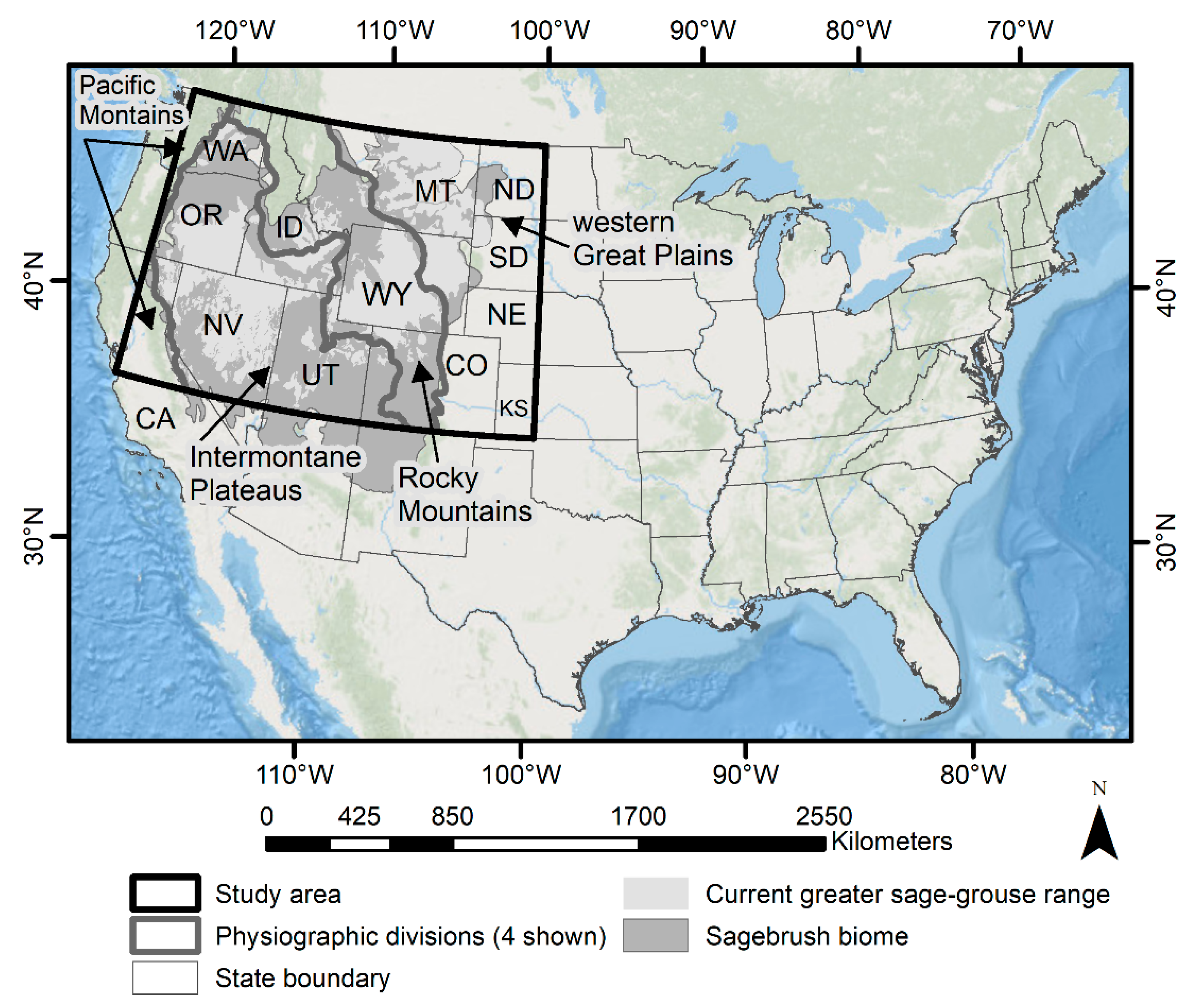
Figure 2.
Workflow describing our implementation of the Newhall simulation modeling framework that we applied to the western United States for climate normals (1981–2010). Beginning at the top and working down, we describe the initial procurement of the data input used in the model, the pre-processing (data input modifications), the modifications made within the Newhall simulation model software (spatial_nsm), the general workflow of the Newhall simulation model and the post-processing steps used for evaluating soil-climate products. AWC = available water capacity; SCAN = soil climate analysis network.
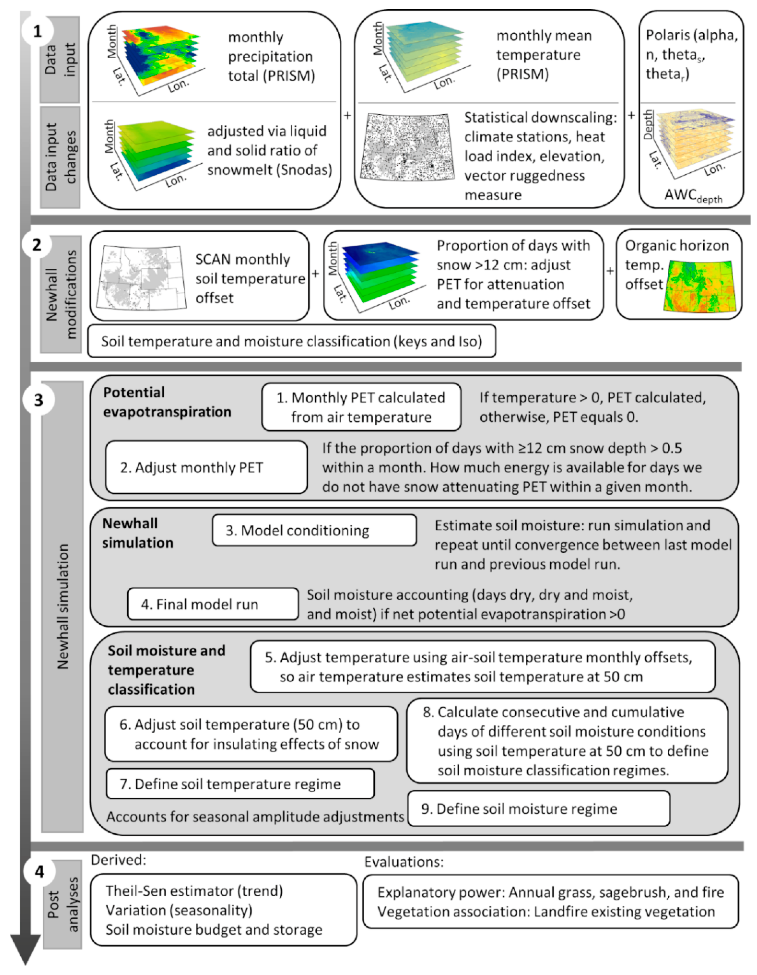
Figure 3.
Effects of snow accumulation and melt demonstrated by “adjusted” versus “unadjusted” precipitation [94] (1981 to 2010 average), where the latter does not differentiate between liquid/solid forms of precipitation. Panel (a) illustrates precipitation data (unadjusted) minus adjusted precipitation (March) and highlights three watershed boundaries (hydrologic unit code [HUC] 12) [165]. Panel (b) is a schematic illustrating how snow water equivalency is released during spring melt. The three histograms (panels (c–e)) show mean differences of unadjusted and adjusted precipitation within example watersheds, demonstrating the importance of considering snowmelt. The current range of greater sage-grouse (Centrocercus urophasianus) occurs within the sagebrush biome and captures the best remaining intact sagebrush.

Figure 4.
Monthly (panels (a–l): March–December) seasonal soil moisture (mm) within the western United States under normal climate conditions (1981–2010).
Figure 4.
Monthly (panels (a–l): March–December) seasonal soil moisture (mm) within the western United States under normal climate conditions (1981–2010).
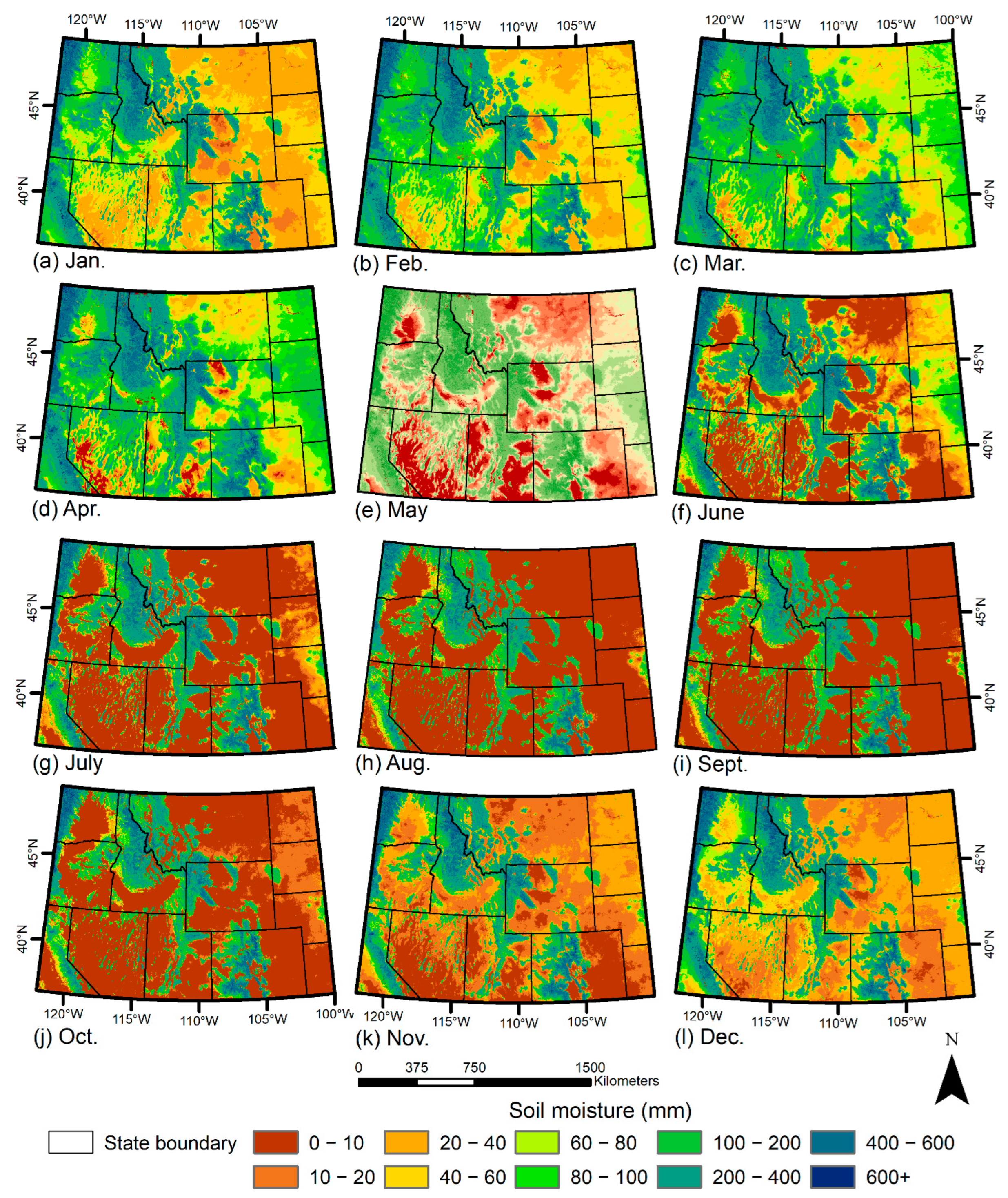
Figure 5.
Assessments of change (Theil–Sen estimator at a 90% confidence interval [CI]) in soil moisture (mm) were estimated within the western United States under normal climate conditions (1981–2010). The median slope of the Theil–Sen estimator from March to June (a) and March to September (b) reflects an increase and decrease in soil moisture across the landscape.

Figure 6.
Seasonality (variability among seasonal moisture [mm]) within the western United States under normal climate conditions (1981–2010). Panel (a) denotes the standard deviation in soil moisture among the four seasons (spring, summer, fall and winter). Panel (b) denotes the standard deviation in the spring growing season (March, April, May and June).

Figure 7.
Combined soil-climate (temperature and moisture) regime classification, where soil moisture and temperature predictions were applied within the western United States and based on normal climate conditions (1981–2010). Colors randomly assigned to combinations of soil temperature, moisture and moisture sub-class; colors are not shown in the legend due to too many combinations. Therefore, this illustration denotes the patterns of soil-climate classifications but does not define or associate the classifications with specific colors.

Figure 8.
Soil temperature-moisture regimes (STMRs) based on averaged climate (1981–2010) and ranked using the estimated abundance of annual herbaceous (ANHB) plants [156] in each type. The classes with the highest mean cover of annual herbs are in dark magenta (≥15% cover within 30 m pixels; Mesic dry xeric to Mesic wet udic); light magenta through yellow and light green represent 10–15% (Mesic typic tempustic to Cryic typic udic); and the least affected classes are in shades of green (<10%; Frigid dry tempudic to Thermic extreme aridic).
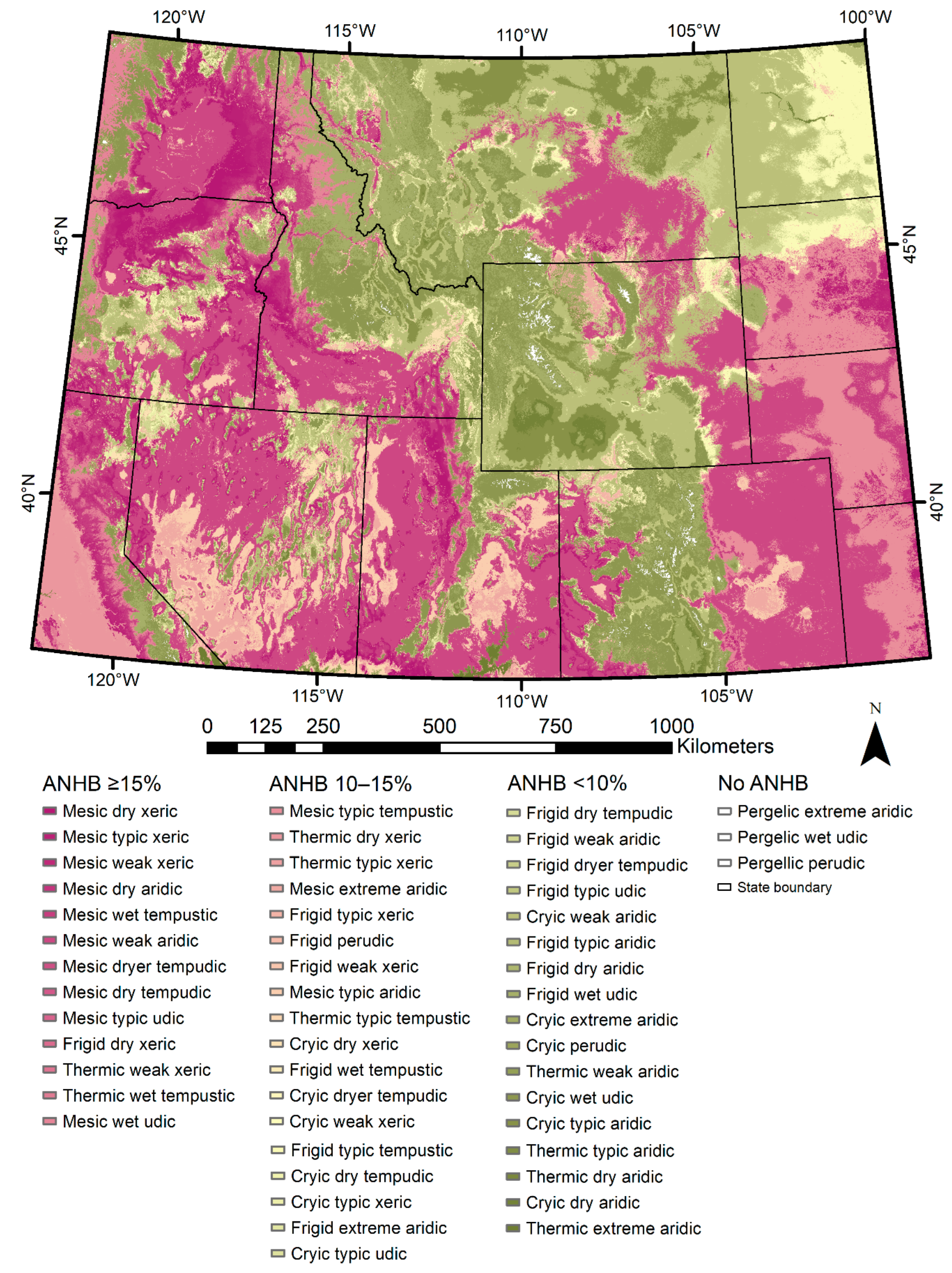
Figure 9.
Comparison mean of fire occurrence (1984–2016; Landsat burned area essential climate variable [BAECV]) [160] and trend were estimated by the Theil–Sen slope in soil moisture across the growing season (March through September). A strong negative trend in soil moisture (x-axis) indicates high moisture early in the season and low moisture late in the season, and these conditions are associated with the highest average fire frequency (top left). For example, aridic soil-climate types, observed in the bottom-right, had a very low fire frequency.


Table 1.
Monthly climate normals (1981–2010) associated with our study area (western United States sagebrush biome) and based on climate stations available from the National Climate Data Center [89] to describe the general climate ranges within our study area. The data include the averages and standard deviation (sd) of precipitation totals (mm) and the minimum (min), maximum (max) and mean temperatures (°C) across stations within the study area. We used 1281 and 1507 climate stations for summarizing precipitation and temperature, respectively.
| Precipitation (mm) | Temperature (°C) | |||||||
|---|---|---|---|---|---|---|---|---|
| Month | Min | Max | Mean | sd | Min | Max | Mean | sd |
| Jan | 2.03 | 463.30 | 34.50 | 50.30 | −15.17 | 10.06 | −3.36 | 4.10 |
| Feb | 1.52 | 346.71 | 30.59 | 41.69 | −12.17 | 11.83 | −1.41 | 4.02 |
| Mar | 5.59 | 319.02 | 36.82 | 36.13 | −6.78 | 14.28 | 3.07 | 3.38 |
| Apr | 6.60 | 210.82 | 38.58 | 22.76 | −3.50 | 16.94 | 7.49 | 0.82 |
| May | 4.83 | 174.75 | 49.94 | 23.00 | 1.83 | 22.39 | 12.47 | 2.81 |
| Jun | 1.27 | 142.75 | 44.51 | 26.21 | 7.50 | 27.50 | 17.15 | 3.01 |
| Jul | 0 | 102.87 | 34.74 | 23.12 | 11.06 | 31.06 | 21.01 | 2.98 |
| Aug | 0.25 | 117.35 | 30.67 | 19.44 | 10.00 | 30.00 | 20.24 | 2.87 |
| Sep | 4.06 | 119.63 | 29.38 | 14.09 | 6.22 | 25.28 | 15.22 | 2.87 |
| Oct | 5.59 | 279.4 | 34.12 | 24.34 | 0.17 | 19.33 | 8.75 | 2.84 |
| Nov | 4.06 | 515.11 | 36.27 | 48.43 | −6.94 | 13.17 | 1.83 | 3.13 |
| Dec | 3.30 | 436.12 | 36.59 | 50.60 | −12.50 | 10.00 | −3.35 | 3.74 |
Table 2.
A comparison of methods for implementing the Newhall simulation model employed by previous research and our research to identify a few of the major modifications we implemented.
Table 2.
A comparison of methods for implementing the Newhall simulation model employed by previous research and our research to identify a few of the major modifications we implemented.
| Description | Previous Research | Our Research |
|---|---|---|
| Soil data 1 | SSURGO/STATSGO | Dynamic |
| Available water capacity | No—use a default of 200 mm | Yes |
| Soil moisture (seasonal, monthly and growing season) | No | Yes |
| Accounting for effects of snow: | ||
| (a) snowmelt depletion curves | No | Yes |
| (b) attenuation of evaporation | No | Yes |
| (c) insulation and offset of soil temperature | No | Yes |
| Accounting for temporal fluctuations of soil temperature | No—use a standard offset of 2.5 °C | Yes |
| Accounting for effects of organic horizon | No | Yes |
| Soil-climate classification | Yes, but java code not always producing classification | Yes |
| Classification of Iso temperature regimes between tropical and temperature soils | Yes, using summer and winter months | Yes, using the three coldest and the three warmest months [129] |
| Model convergence and number of iterations to achieve moisture at 30 December being <1/100th of the moisture on 30 December of the preceding iteration | ≤10 iterations (convergence not always achieved) | ≤1000 iterations (convergence achieved) |
| Accounting for root zone depth 2 | No | Partially, with mask (see Supplemental Materials) |
| Accounting for the influence of groundwater on soil moisture | No | No, but less of a factor in rangelands |
| Accounting for soils with lateral inflows or outflows of water | No | No |
1 A few previous research methods applied within the United States included the use of gridded soil data (U.S. Department of Agriculture Natural Resources Conservation Service [NRCS] products: Soil Survey Geographic Database [SSURGO] and State Soil Geographic Database [STATSGO2]) characterizing soil-climate regimes [130,131] and the use of gridded soil data (SSURGO/STATSGO2) with gridded climate data (Parameter-elevation Regressions on Independent Slopes Model [PRISM] 4 km) using the NRCS java Newhall simulation model [100,132,133]. 2 We have not identified any spatial data that sufficiently map root zone depth. Some products exist for identifying depth to bedrock [134,135], but these depths will have almost no effect on our results because they are not providing information on soil pans or shallower depths.
Table 3.
Comparison of the volumetric water content (soil moisture as m3m−3) measured at 209 stations associated with SCAN [147] and snow telemetry (SNOTEL) [148] networks (1996–2010 observations at 50 cm depth) to Newhall simulation model estimates using two soil profiles and the Thornthwaite–Mather-Sellers potential evapotranspiration equation. The two soil profiles reflected our soil moisture results of 0–200 cm, and we also compared estimates using 30–60 cm Polaris available water capacity (AWC) data.
| Polaris (0–200 cm) | Polaris (30–60 cm) | |||||
|---|---|---|---|---|---|---|
| Month | Pearson’s r | p-Value | Ubrmse (m3m−3) | Pearson’s r | p-Value | Ubrmse (m3m−3) |
| Jan | −0.0102 | 0.8933 | 0.1238 | −0.0811 | 0.286 | 0.1124 |
| Feb | −0.0263 | 0.7293 | 0.1247 | −0.1131 | 0.1362 | 0.1144 |
| Mar | −0.0489 | 0.5201 | 0.1279 | −0.1451 | 0.0553 | 0.1203 |
| Apr | −0.0989 | 0.1928 | 0.1343 | −0.1706 | 0.024 | 0.1255 |
| May | −0.0393 | 0.6056 | 0.127 | −0.0922 | 0.2248 | 0.1188 |
| Jun | 0.0521 | 0.4933 | 0.1467 | 0.1796 | 0.0174 | 0.135 |
| Jul | 0.098 | 0.197 | 0.1632 | 0.2466 | 0.001 | 0.1535 |
| Aug | 0.0207 | 0.7862 | 0.1347 | 0.2007 | 0.0078 | 0.1208 |
| Sep | 0.0338 | 0.6574 | 0.1211 | 0.2799 | 0.0002 | 0.105 |
| Oct | 0.0728 | 0.3385 | 0.1202 | 0.224 | 0.0029 | 0.1062 |
| Nov | 0.047 | 0.5372 | 0.1214 | 0.0509 | 0.5039 | 0.1095 |
| Dec | 0.0105 | 0.8906 | 0.1215 | −0.0678 | 0.3726 | 0.1103 |
Publisher’s Note: MDPI stays neutral with regard to jurisdictional claims in published maps and institutional affiliations. |
© 2022 by the authors. Licensee MDPI, Basel, Switzerland. This article is an open access article distributed under the terms and conditions of the Creative Commons Attribution (CC BY) license (https://creativecommons.org/licenses/by/4.0/).
Share and Cite
MDPI and ACS Style
O’Donnell, M.S.; Manier, D.J. Spatial Estimates of Soil Moisture for Understanding Ecological Potential and Risk: A Case Study for Arid and Semi-Arid Ecosystems. Land 2022, 11, 1856. https://doi.org/10.3390/land11101856
AMA Style
O’Donnell MS, Manier DJ. Spatial Estimates of Soil Moisture for Understanding Ecological Potential and Risk: A Case Study for Arid and Semi-Arid Ecosystems. Land. 2022; 11(10):1856. https://doi.org/10.3390/land11101856
Chicago/Turabian StyleO’Donnell, Michael S., and Daniel J. Manier. 2022. "Spatial Estimates of Soil Moisture for Understanding Ecological Potential and Risk: A Case Study for Arid and Semi-Arid Ecosystems" Land 11, no. 10: 1856. https://doi.org/10.3390/land11101856
Note that from the first issue of 2016, this journal uses article numbers instead of page numbers. See further details here.