Soil Moisture and Water Transport through the Vadose Zone and into the Shallow Aquifer: Field Observations in Irrigated and Non-Irrigated Pasture Fields

Abstract

Reliable estimates of soil moisture and other field observations (e.g., precipitation, irrigation) are critical to quantify the seasonal variability of surface water and groundwater relationships. This is especially important in pasture-based agroecosystems that rely on surface water diversions and precipitation inputs for agricultural production. The objectives of this study were to (1) quantify soil water balance components in irrigated and non-irrigated pasture fields in western Oregon, USA and (2) evaluate soil moisture and shallow aquifer recharge relationships in irrigated vs. non-irrigated pasture fields. Four monitoring stations in each field were used to measure soil water content in the upper 0.8 m profile and shallow groundwater levels. A soil water balance (SWB) approach was used to determine deep percolation based on field measurements of several other hydrology variables (e.g., irrigation and soil moisture). The water table fluctuation method (WTFM) was used to estimate shallow aquifer response to irrigation and precipitation inputs. Results from this study add to the understanding of seasonal water transport through the vadose zone and into the shallow aquifer in agroecological systems with fine-textured soils in the Pacific Northwest region of the United States.

1. Introduction

Large portions of the western United States are experiencing prolonged drought, extended water deficits, and threats to ecosystem resilience [1,2] and socioeconomic systems [3,4]. Shifts in the type and timing of precipitation [5] and reduced snowpack [6] are creating uncertainty in soil moisture annual cycles [7], which impact groundwater recharge [8] and complicate water management due to decreased surface water supplies and increased reliance on groundwater use [9].

Disruption of the water cycle is especially concerning in the Pacific Northwest region in the USA as decreased streamflow place substantial pressure on multiple issues, such as water management and water allocation between agriculture [10], wildfire suppression [11], aquatic ecosystem requirements [12] and hydropower uses [13].

The Willamette Valley in western Oregon, part of the Pacific Northwest region, is home to over 60% of the State of Oregon’s population and is a rich agricultural area used for crop production and pastureland [14]. Grazing is common, as cattle and calves are the second-highest agricultural commodity in the state [15]. Most pasture lands in the Willamette Valley are not irrigated and rely on winter precipitation for plant growth during the spring and summer before soils dry out, making them sensitive to shifts in the timing, type, and amount of precipitation [16]. Rainfall precipitation and summer irrigation are important indicators of soil moisture variability, which in turn can affect forage growth [17,18], field-water budgets [19], and groundwater recharge [20].

To ensure pastureland forage production is efficient, low-cost, and high-quality to be as resistant to weeds and drought as possible, water managers and farmers require a better understanding of surface water and groundwater relations [21]. Accurate quantification of field water budget components is needed to inform water management decisions affecting the supply and timing of irrigation, soil water transport, groundwater recharge, and groundwater return flows [22,23]. Precipitation is a significant source of groundwater recharge and is essential for long-term aquifer replenishment [24,25] as soils become saturated and soil water percolates past the vadose zone into the aquifer. Groundwater recharge also elevates the water table, which benefits crop water use if a higher soil moisture content is maintained [26]. In addition to increasing soil moisture content, irrigation may impact surface water-groundwater (SW-GW) interactions [27] by recharging shallow aquifers through deep percolation and providing irrigation return flows to adjacent streams [28,29,30].

Groundwater recharge can be estimated using procedures such as a soil water balance (SWB) assessment and the water table fluctuation method (WTFM) [31,32]. When using an SWB approach, estimates of deep percolation, calculated as the residual of soil water inputs and outputs, are equated to potential groundwater recharge, assuming that water percolating below the plants’ root zone will reach the aquifer. Various investigations have used deep percolation to calculate aquifer recharge through irrigation [28,33,34] and precipitation [35,36,37]. The physical characteristics of the soil highly impact deep percolation, water extraction patterns by roots, surface ponding time, and water table depth [38,39]. Soils with high clay content have greater field capacity, which increases soil water storage and reduces transmissivity [40,41]. In contrast, clayey soil’s drying and wetting cycles can create cracks, or macropore pathways, throughout the soil profile that provide an avenue for water, nutrients, and contaminants to reach the water table [42].

The WTFM assumes rises in the water table are caused by actual recharge (Re) of the aquifer, mainly from irrigation [43] and precipitation [35]. This method is frequently used because water table depth is relatively easy to measure [32,44]. Re is calculated as the product of the rises in groundwater level and the specific yield (Sy) of an unconfined aquifer, where Sy describes the capacity of the aquifer substrate to yield water to gravity [32]. Limitations of the WTFM are determining an accurate Sy value for a particular aquifer since Sy values vary by depth and may not be constant [44,45,46].

Annual and seasonal variations in SW-GW interactions and soil moisture cycles, as impacted by irrigation and precipitation, have not been fully explored in clayey pasture fields of the Willamette Basin. This investigation utilized soil texture and bulk density, soil moisture content, and groundwater level fluctuations to characterize seasonal soil water movement through the vadose zone and into the shallow aquifer in a non-irrigated, non-livestock-grazed pasture field and in an irrigated, livestock-grazed pasture field in the Willamette Valley. The objectives of this study were to (1) quantify soil water balance components in irrigated and non-irrigated pasture fields in western Oregon, USA and (2) evaluate soil moisture and shallow aquifer recharge relationships in irrigated vs. non-irrigated pasture fields.

2. Materials and Methods

2.1. Site Description

This study was conducted for two consecutive years (Yr1 and Yr2). Yr1 ran from 1 April 2020 to 31 March 2021, and Yr2 from 1 April 2021 to 31 March 2022. The study area comprised a 2.1 ha irrigated pasture field (IRR_FLD) and a 2.9 ha non-irrigated pasture field (N_IRR_FLD) located at the Oregon State University (OSU) Dairy Center in Corvallis, Oregon, USA. The IRR_FLD is located north of Oak Creek, while the N_IRR_FLD is located south of Oak Creek, with the fields being approximately 350 m from each other (Figure 1). The IRR_FLD is cattle grazed and irrigated during the summer, with surface water pumped from Oak Creek. Field vegetation includes a mix of balansa clover (Trifolium michelianum balansae), perennial ryegrass (Lolium perenne), and common chicory (Cichorium intybus) [47]. According to the USDA official series description, dominant soils are Bashaw clay (55.8% of the field) and Holcomb silt loam (44.2% of the field), with slope values between 0% to 3%. Bashaw clay falls within the ‘poorly drained’ category, and the Holcomb silt is within the ‘somewhat poorly drained’ category. During the winter season, the average depth to the water table ranges between 0 to 76 mm [48]. The N_IRR_FLD is typically used for grass silage production with one cutting annually and is mostly covered by annual ryegrass (Lolium multiflorum). Bashaw silty clay loam covers 100% of the field with slope values of 0% to 3%. The average depth to the water table during the winter season ranges from 0 to 127 mm, and the drainage class is categorized as ‘poorly drained’ [48].

The Willamette Valley has a Mediterranean type of climate with a warm, dry summer season and cool, wet winter season. Most precipitation falls as rain between November and April with mean annual precipitation ranging from 1000 mm in the Valley, where the study site is located, to 2500 mm at higher elevations. Total monthly averaged precipitation is highest in December (181.4 mm) and lowest in July (9.1 mm). Monthly averaged temperature ranges from 0.67 °C in January to 27.4 °C in August [49].

Table 1. Average monthly precipitation (mm), average daily maximum, and average daily minimum temperature (°C) for the period of record 1 October 2016 to 30 September 2022 in Corvallis, OR, USA. (Source: https://www.usbr.gov/pn/agrimet/agrimetmap/crvoda.html; accessed on 6 November 2022).

Month	Precipitation	Daily Maximum Temperature	Daily Minimum Temperature
October	103	17.4	6.3
November	138	12.4	4.1
December	150	8.1	1.2
January	148	9.0	2.0
February	122	9.5	1.2
March	91	12.9	2.4
April	92	16.1	4.6
May	48	20.5	7.3
June	38	24.3	10.2
July	3.3	29.1	11.6
August	1.8	29.5	12.1
September	46	24.8	10.4

shows the seasonal variability of precipitation and temperature in the region.

2.2. Field Soil, Water, and Weather Data Collection

Multiple monitoring stations were used to collect hourly groundwater level, soil moisture, and weather data to calculate field water budget components, determine shallow aquifer recharge, and analyze soil moisture cycles during the two-year study period. A weather station installed in an adjacent field measured various weather parameters (e.g., air temperature, relative humidity, wind speed and direction, solar radiation) to output reference evapotranspiration, ET_o, values. The weather station was programmed to calculate ET_o hourly using the ASCE Standardized Reference Evapotranspiration Equation [50]. Each experimental field had four soil moisture and groundwater level monitoring stations, each equipped with a vertical network of three soil sensors (Model CS655, Campbell Scientific, Inc.; Logan, UT, USA) placed at 0.2, 0.5, and 0.8 m depths. The monitoring stations were installed in all cardinal directions (North, South, West, and East) to capture the spatial variability of the parameters monitored at each field. The soil sensors were connected to a CR300 RF407 datalogger (Campbell Scientific, Inc.; Logan, UT, USA) and were programmed to record hourly soil volumetric water content (θ) data. The variability of θ within and below the effective root zone (ERZ), defined as 0 to 0.6 m given the shallow-rooted vegetation in both fields, were assessed using data from the sensors installed at 0.2 and 0.5 m (within the ERZ) and 0.8 m (below the ERZ). Soil bulk density (ρb) and soil texture were analyzed using three soil samples collected at each sensor depth at the time of sensor installation in 2018 for all stations in the N_IRR_FLD and 2018 (West and East), 2019 (North), and 2020 (South) in the IRR_FLD. Soil texture was determined using the hydrometer method [51], while ρb was determined using the core method [52]. Based on the USDA soil classification, θ at field capacity (θ_FC) for the different sensor depths (i.e., 0.2. 0.5, and 0.8 m) was estimated using the Soil Web Survey tool [48]. The θ_FC values for the Holcomb silt loam were 29.6% for 0 to 0.2 m, 29.3% for 0.2 to 0.5 m, and 36.6% for 0.5 to 0.8 m. For the Bashaw clay, θ_FC values were 44.8% for 0 to 0.2 m, 45.2% for 0.2 to 0.5 m, and 45.2% for 0.5 to 0.8 m. It was assumed that θ values exceeding FC would percolate to the next soil layer.

2.2.1. Runoff

Efforts to directly measure runoff out of the fields were unsuccessful due to equipment malfunctioning. Therefore, runoff was calculated using the SCS-CN method [53]. This empirical equation predicts runoff from rainfall and uses an S parameter based on land use, vegetation, soil texture, and soil moisture.

$$RO=\frac{{\left(P-0.2S\right)}^2}{\left(P+0.8S\right)} \mathrm{for} P>0.2S,$$

(1)

$$RO=0 \mathrm{for} P\le 0.2S,$$

(2)

where RO = runoff (mm); P = precipitation (mm); and S = retention parameter (mm). The value of S is calculated using the following equation:

$$S=\frac{25,400}{{\mathrm{CN}}_{3\mathsf{\alpha }}}-254,$$

(3)

The value of CN is determined by the hydrologic soil group, land cover, and management type using a table from the SCS handbook [53]. Based on topographic surveys conducted, the slope, α, for the IRR_FLD was 0.012 and 0.0065 for the N_IRR_FLD. An α factor was incorporated into the following equation, as described in [54], to obtain slope correction RO values;

$${\mathrm{CN}}_{3\mathsf{\alpha }}=\frac{1}{3}\left({\mathrm{CN}}_3-{\mathrm{CN}}_2\right)\left(1-2{\mathrm{e}}^{-13.86\mathsf{\alpha }}\right)+{\mathrm{CN}}_2,$$

(4)

where CN₂ = average soil moisture conditions; CN₃ = wet soil moisture conditions; and α = slope. CN₂ and CN₃ values were obtained from the runoff curve numbers for other agricultural lands (pasture) reported in [55]. Since RO was only observed after the soil reached saturation, a wet soil condition correction was used on the slope-corrected CN (CN_3α) value. A CN_3α value of 88 was used for both experimental fields, resulting in an S value of 34 for the IRR_FLD and 36 for the N_IRR_FLD (Equation (3)).

2.2.2. Irrigation Applied

As described in [43], the IRR_FLD was irrigated using a pod sprinkler system (© K-Line North America 2016) with two lines of 8 and 9 sprinkler pods extending from two irrigation pipe risers in the center of the field. The 2020 irrigation season started on 27 July and ended on 12 September, while the 2021 season ran from 15 June to 9 September. The amount of water applied for each irrigation event was calculated based on volume measurements using water collectors and added for the entire irrigation season. The late start of the irrigation season in year 2020, due to complications with irrigation pipe system, resulted in less irrigation events (n = 6) than in year 2021 (n = 13). The total amount of irrigation recorded at each station in 2020 ranged from 214 mm in the West station to 280 mm in the East Station. In 2021, total irrigation ranged from 368 mm in the North station to 391 mm in the South station. The IRR_FLD was divided into four smaller subplots; each plot was irrigated for 48 h at the beginning of the season when soil conditions were dry and then switched to 24 h once ponding began to prevent runoff. Approximately 29 mm of irrigation water were applied to each subplot in a 24 h irrigation cycle each week [43]. The weekly frequency of irrigation and amount of water applied each week was consistent with pod sprinkler applications in several other neighboring fields.

2.2.3. Groundwater Levels

Each monitoring station was equipped with a shallow monitoring well (50 mm diameter) made out of PVC with 3.5 m of solid pipe and a 1.5 m screen section on the bottom. Each well was equipped with a CTD-10 water level sensor (Decagon Devices, Inc.; Pullman, WA, USA) connected to the CR300 datalogger to collect hourly groundwater level data. A topographic survey was conducted to determine the elevation of the groundwater level and soil surface. Information from this survey and hourly records of groundwater levels were used to calculate daily and seasonal groundwater variability in each well.

2.3. Soil Water Balance (SWB)

A soil water balance approach was utilized to calculate deep percolation, defined as water that percolated below the 0.8 m sensor depth and was assumed to reach the shallow aquifer as it was no longer subject to root extraction within the ERZ.

DP = IRR + P − RO − Δθ − AET,

(5)

where DP = deep percolation (mm); IRR = irrigation depth (mm); P = precipitation (mm); RO = field runoff (mm); ∆θ = change in soil water storage (mm); and AET = actual evapotranspiration (mm). Hourly measurements of the various parameters (e.g., soil moisture) were converted to daily estimates of SWB components, then averaged for all stations in each pasture field. AET was calculated using reference ET_o estimates obtained from the onsite weather station, and pasture crop coefficient (K_c) values (0.25 to 0.68) as reported by the Columbia-Pacific Northwest Region USDA Agriculture Research Service [56]. The pasture-grass growth cycle used in calculating AET was determined using bi-monthly (twice a month) growth periods described in Fransen et al. [57] which was then associated with a specific K_c value. RO was calculated using the SCS-CN [53] method with a slope correction (Equation (4)) [54].

Daily SWB calculations were averaged by station and aggregated for each month and quarter for Yr1 and Yr2. The 1st quarter (Apr–Jun) was defined as 1 April to 30 June; the 2nd quarter (Jul–Sep) was 01 July to 30 September; the 3rd quarter (Oct–Dec) 1 October to 31 December; and the 4th quarter (Jan–Mar) was 1 January to 31 March. The field water budget components evaluated are illustrated in Figure 2.

2.4. Shallow Aquifer Recharge

Hourly groundwater level data for each monitoring well, and the WTFM were used to estimate yearly shallow aquifer recharge (Re, mm).

$$Re=\frac{\Delta h}{\Delta t}\times Sy$$

(6)

where Re = aquifer recharge (mm) for a given time; ∆h/∆t = fluctuation in groundwater level (mm) for a given time; and Sy = specific yield of the unconfined aquifer. Based on the methods described in Sophocleous [32], Sy values were calculated by aggregating the daily potential recharge values (i.e., DP) to get monthly values and dividing the monthly aggregated daily rises in groundwater level at each station. The monthly averaged Sy values used for the IRR_FLD were from November 2020 (0.09) and October 2021 (0.06). These months were selected because they showed rapid rises in θ at the three sensor depths and groundwater level, indicating that water percolated through the vadose zone into the aquifer. The relatively quick groundwater level response to precipitation or irrigation observed is similar to the conditions recommended by Sophocleous [32] when deciding on data to use in the WTFM. A mean Sy value of 0.08 was calculated, similar to the 0.06 Sy value for the irrigation season alone and previously reported by Gómez et al. [43] and the Sy value shown in Dingman [58] for clay soils.

2.5. Statistical Analyses

Linear regression analyses were conducted to determine the relationships between water outputs (RO and AET) and TWA-Δθ (antecedent θ) with DP and to examine which component had the most influence on seasonal DP. Kendall rank correlation coefficients were used to determine the correlation between water outputs and TWA-Δθ with DP. A Kruskal–Wallis One-Way Analysis of Variance ranks (ANOVA) was conducted to assess the differences in groundwater levels for the eight monitoring wells. A Kruskal–Wallis ANOVA was also conducted to determine the relationship between ∆θ and DP for the two study sites and the irrigation and rainy winter seasons. An α value of 0.05 was used for all analyses to determine significant differences. The R statistical software was used for all statistical analyses [59].

3. Results

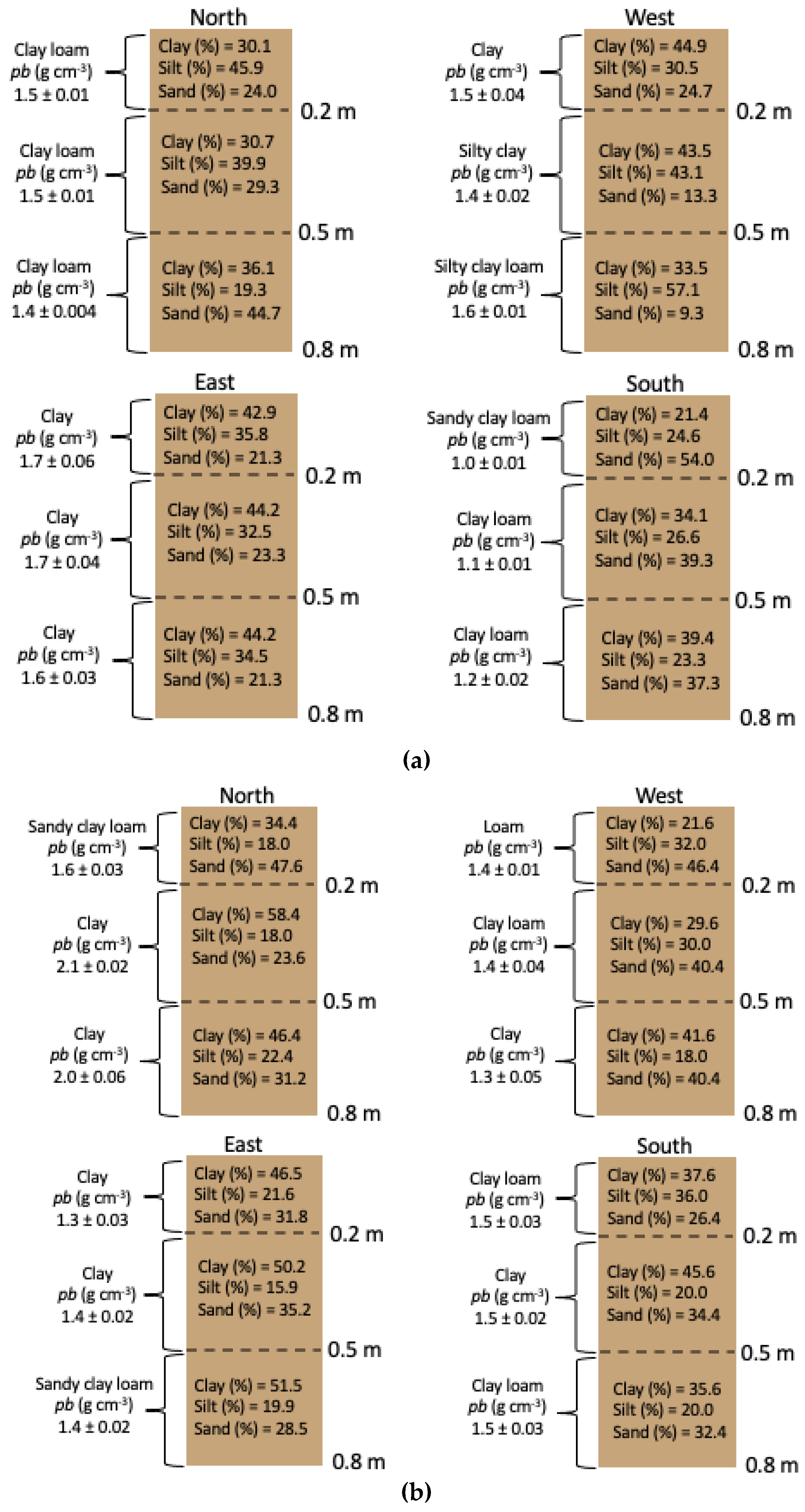
3.1. Soil Properties

Soil physical properties for both experimental fields varied between monitoring stations and sensor depths (Figure 3). Gómez et al. [43,60] reported that the IRR_FLD had clay soils at all depths in the East station and 0.2 m deep at the West station. These two stations had the highest average ρb values (1.7 g cm⁻³ and 1.5 g cm⁻³) along with the North station (1.5 g cm⁻³), which had clay loam soils at all depths. For the South station, coarser soils were found at the 0.2 m depth and loamy soils at the bottom two depths (0.5 and 0.8 m). This station had the lowest mean ρb (1.1 g cm⁻³). In the N_IRR_FLD, coarser-texture soils were found at the top 0.2 m across the field, except for the East Station, and clay soils at the 0.5 m depth in all stations. Clay soils were found at 0.8 m in the West and North station, whereas loamy soils were seen at the same depth in the South and East stations. The West and East stations had the lowest ρb (1.4 g cm⁻³ for both), and the North and South stations had the highest ρb (1.9 g cm⁻³ and 1.5 g cm⁻³, respectively) (Figure 3).

3.2. Soil Water Balance Method

The SWB calculations by quarter and year for the IRR_FLD and N_IRR_FLD are shown in

Table 2. Quarterly and total by year (in mm) portioning of the various water budget components for the irrigated (IRR_FLD) and non-irrigated (N_IRR_FLD) fields. Water budget components are precipitation (P), irrigation (IRR), total change in soil water storage (∆θ), actual evapotranspiration (AET), runoff (RO), and deep percolation (DP).

	IRR_FLD						N_IRR_FLD
Year (Quarter)	P	IRR	∆θ	AET	RO	DP	∆θ	AET	RO	DP
Yr1 (Apr–Jun)	138	0	−70	161	0	174	−117	172	0	157
Yr1 (Jul–Sep)	48	249	120	207	0	100	−70	144	0	39
Yr1 (Oct–Dec)	377	0	12	37	114	300	184	34	43	268
Yr1 (Jan–Mar)	450	0	−8	32	149	382	−7	32	85	391
Yr1 Total	1013	249	54	438	263	956	−10	383	135	855
Yr2 (Apr–Jun)	42	74	−16	222	0	55	−203	209	0	139
Yr2 (Jul–Sep)	48	308	152	195	0	96	−16	153	0	24
Yr2 (Oct–Dec)	566	0	14	28	164	462	227	26	108	440
Yr2 (Jan–Mar)	276	0	−6	34	117	220	−8	34	64	239
Yr2 Total	932	381	144	479	281	833	0	423	172	841

. Overall, higher P and DP were observed in Yr1 than in Yr2. P was measured in an adjacent field; thus, it was considered the same for both experimental fields. The portioning of annual DP to total water applied (P + IRR) in the IRR_FLD was 76% in Yr1 and 63% in Yr2. Annual IRR to the total water applied was 20% in Yr1 and 29% in Yr2. For the N_IRR_FLD, DP represented 84% of total P in Yr1 and 90% in Yr2.

Annual AET and RO were higher in the IRR_FLD than in the N_IRR_FLD in both years. Quarterly AET values were significantly higher in the spring and summer in both fields. Conversely, quarterly RO values were substantially higher in the fall and winter. Total AET represented 35% and 38% of total water applied in the IRR_FLD in Yr1 and Yr2, respectively. For the N_IRR_FLD, annual AET was 38% of total P in Yr1 and 45% in Yr2. When it occurred, quarterly RO was significantly higher in the IRR_FLD than in the N_IRR_FLD.

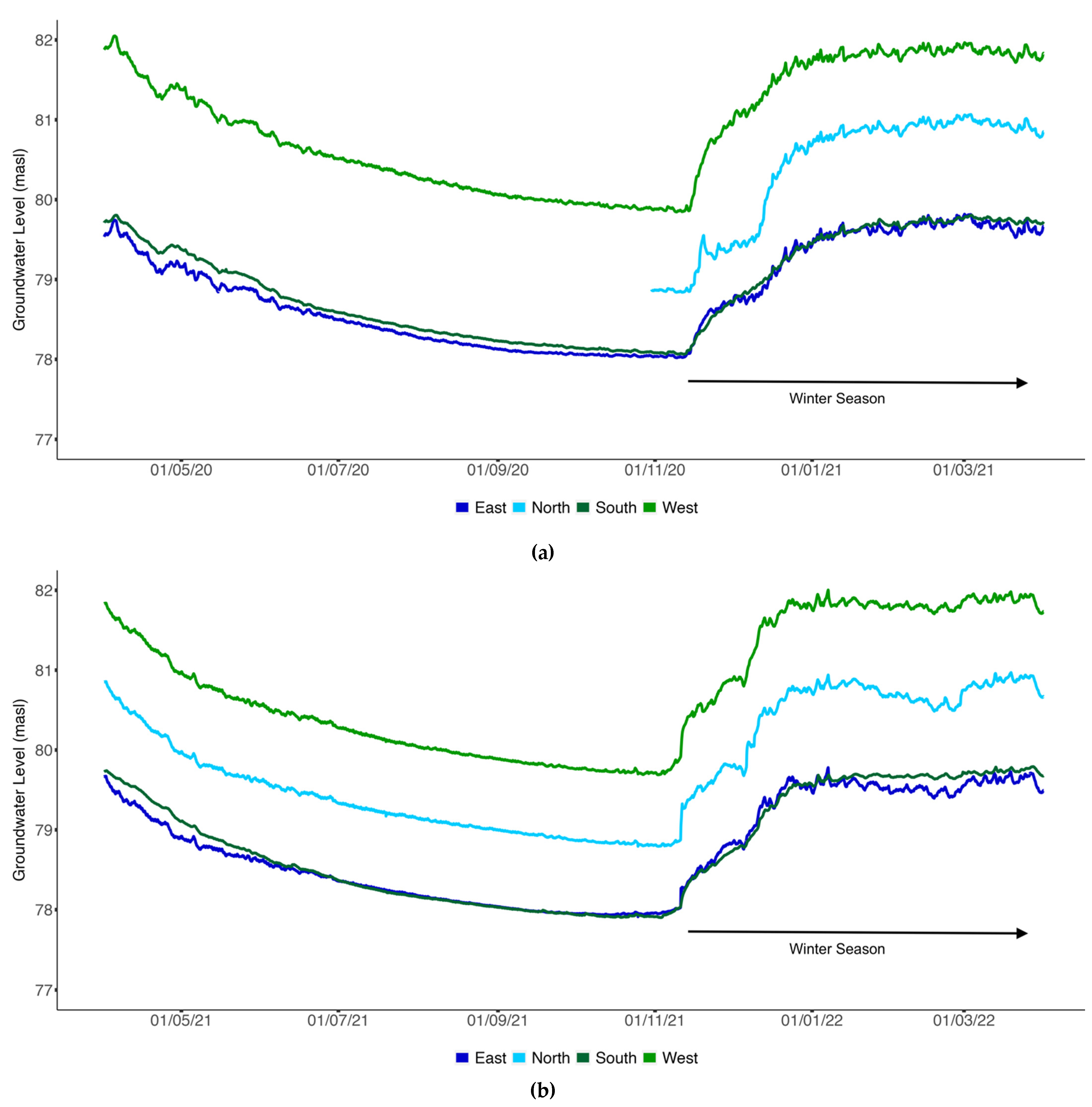
3.3. Groundwater Level Variability and Aquifer Recharge

Groundwater level response differed between the IRR_FLD (Figure 4a,b) and the N_IRR_FLD (Figure 5a,b). In both years, rapid rises in groundwater levels were observed in the IRR_FLD shallow aquifer due to irrigation events that led to DP, with the groundwater level subsiding before the next irrigation event. In contrast, no rapid rises in the groundwater level were observed in the N_IRR_FLD during the summer months (DP = 0), causing the groundwater level in all four monitoring stations to drop throughout the summer until the start of the winter season. The groundwater level in both fields responded the most to precipitation inputs during the winter season, which maintained an elevated groundwater level throughout the winter with small fluctuations between storms before decreasing around March until the start of the next irrigation season (IRR_FLD) or until the next winter season (N_IRR_FLD). At the beginning of the winter, the groundwater level of the IRR_FLD responded before the N_IRR_FLD. This is likely due to the IRR_FLD having higher soil moisture levels before the rains began due to previous irrigation applied.

In contrast, the soils in the N_IRR_FLD needed to reach saturation before the rainfall infiltrated the shallow aquifer. During the winter, the average groundwater level rise in the IRR_FLD was 2048 mm in Yr1 and 1727 mm in Yr2. For the N_IRR_FLD, the average groundwater level rise was 1964 mm in Yr1 and 2144 mm in Yr2.

Annual Re estimates varied by year for the IRR_FLD (289 mm in Yr1 vs. 451 mm in Yr2) but were more consistent in the N_IRR_FLD (157 mm in Yr1 vs. 178 mm in Yr2), as shown in

Table 3. Mean seasonal and total aquifer recharge (Re, in mm) and total water applied (TWA = P + IRR, in mm) for each field and year.

	IRR_FLD		N_IRR_FLD
Year—Season	Re	TWA	Re	TWA
Yr1—Irrigation	132	249	0	0
Yr1—Winter	157	1013	157	1013
Yr1—Total	289	1262	157	1013
Yr2—Irrigation	290	381	0	0
Yr2—Winter	161	932	178	932
Yr2—Total	451	1314	178	932

. Yearly Re and total water applied (TWA = P + IRR, in mm) were higher in the IRR_FLD than the N_IRR_FLD. For the IRR_FLD, average Re during the irrigation season (132 mm) was lower than winter season Re (157 mm) for Yr1, but irrigation Re (290 mm) was higher than winter Re (161 mm) during Yr2 [43]. Similarly, during Yr1, the IRR_FLD’s irrigation season Re (132 mm) was lower than the N_IRR_FLD’s winter season Re (157 mm). Despite the N_IRR_FLD having a lower yearly Re than the IRR_FLD, they had identical winter season Re in Yr1 (157 mm), but the N_IRR_FLD had higher winter season Re (178 mm) than the IRR_FLD (161 mm) during Yr2.

3.4. Soil Moisture Variability

Seasonal θ, TWA, and groundwater level trends varied between the two experimental fields (Figure 6a,b). In the IRR_FLD, the winter season rain resulted in rapid soil water infiltration through the soil profile at the three depths (0.2, 0.5, and 0.8 m), with the shallowest sensor generally responding first followed by the two other sensors sequentially in all stations (Figure 6a). The θ values for the entire 0.8 m soil profile stayed near saturation with little variability through the winter season, with θ level declines occurring between rain events. Groundwater levels remained elevated and stable through the winter, with declines occurring between rain events. During the summer, irrigation events increased θ, leading to rapid DP and groundwater Re [43,60]. Since each station was irrigated once a week, this allowed time for the soils to drain and for the groundwater level to drop before the following irrigation event. This led to sharp fluctuations in θ and in groundwater levels that were not observed during the winter.

In contrast, the N_IRR_FLD station trends did not experience rises in θ or groundwater levels during the summer, as the field was not irrigated and only responded to the winter season P inputs (Figure 6b). As the winter season began, the first initial rains only increased θ, while groundwater levels did not rise until the heavier and more consistent rains started (i.e., mid-November 2020 through late March 2021 in Yr1 and early November 2021 through late March 2022 in Yr2). Soil water percolation was evident, with the shallowest θ sensor responding first to a P event, followed by the 0.5 and 0.8 m sensors. The shallowest θ sensor was also the first to drain, followed by the subsequent sensors. Both θ and groundwater levels varied less in the N_IRR_FLD compared to the IRR_FLD. Once the winter season ended, θ and groundwater levels declined continuously until the start of the next winter season.

3.5. Statistical Analyses

Linear regression analyses in both fields revealed that there was a significant (p ≤ 0.05) relationship between TWA-Δθ and water outputs (RO and AET) with DP at the seasonal scale (

Table 4. Quarterly linear regression analysis R² values, Kendall rank correlation coefficient (τ), and p-values for TWA, TWA—Δθ, AET, and RO against DP for the IRR_FLD and the N_IRR_FLD. N represents the sample size.

	IRR_FLD				N_IRR_FLD
Component	R2	τ	p-Value	N	R2	τ	p-Value	N
TWA (P + IRR)	0.79	0.64	0.003	8	0.93	0.84	0.001	8
TWA—Δθ	0.84	0.93	0.001	8	0.74	0.71	0.006	8
AET	0.80	−0.86	0.003	8	0.63	−0.69	0.02	8
RO	0.87	0.91	0.0008	8	0.88	0.81	0.0006	8

). AET had a negative correlation with DP, while RO and TWA-Δθ had a positive correlation with DP. In the IRR_FLD, TWA-Δθ and RO had the strongest correlation with DP followed by AET. For the N_IRR_FLD, RO had the strongest correlation with DP followed by TWA-Δθ and AET. Unlike the irrigation season results reported in Gómez et al. [43], TWA had a significant relationship with DP for both the IRR_FLD and the N_IRR_FLD.

A Kruskal–Wallis One-Way ANOVA on ranks test on groundwater level results showed that all pairwise comparisons between fields and wells were significantly different (p < 0.001, N = 8). DP and Δθ Kruskal–Wallis comparisons between the two fields and the irrigation and rainy winter season showed that there were no significant differences in Δθ (p > 0.05, N = 8), and similar results were found with DP (p > 0.05, N = 8). The two exceptions were between the N_IRR_FLD winter season DP vs. N_IRR_FLD irrigation season DP (p = 0.03) and the IRR_FLD winter season DP vs. N_IRR_FLD irrigation season DP (p = 0.03) where there were significant differences.

4. Discussion

This research examined the variability in field water budget components and shallow aquifer throughout the year in irrigated and non-irrigated pasture fields with fine-textured soils in the Willamette Valley, OR, USA [60]. Rainfall constituted the largest source of water on the fields and led to large and sustained saturated soil conditions and elevated groundwater levels through the winter season. Irrigation water in the IRR_FLD added an average of 25% to the total precipitation estimates. Water percolating (DP) below the upper 0.8 soil profile was calculated using a soil water balance (SWB) approach and was assumed to reach the aquifer. The actual recharge (Re) of the shallow aquifer was estimated using the water table fluctuation method (WTFM). On average, total DP was higher in the IRR_FLD (895 mm year⁻¹) than in the N_IRR_FLD (848 mm year⁻¹). Total annual Re estimates were also higher in the IRR_FLD (371 mm year⁻¹) than in the N_IRR_FLD (168 mm year⁻¹). The relatively high amounts of yearly DP and Re obtained were attributed to a combination of factors including significant amounts of winter precipitation, the added irrigation for the IRR_FLD during the summer, the physical properties of the soil that may have resulted in the potential presence of macropore pathways, and a relatively shallow aquifer. The lower Re estimates in the IRR_FLD (161 mm) than in the N_IRR_FLD (178 mm) during the wintertime in Yr2 were attributed in part to the higher amount of irrigation applied during the summer, which maintained the water table higher, giving less room for more pronounced groundwater level rises at the beginning of the winter precipitation. The significantly higher amount of precipitation in the Oct-Dec quarter, at the end of the irrigation season, in Yr2 (Table 2) might have also contributed to the greater water table response observed in the drier N_IRR_FLD. However, the large differences observed between yearly DP and Re estimates indicate that some of the assumptions used for calculating aquifer recharge with either method (SWB and WTFM) need to be examined more carefully. Another limitation of this study was the lack of direct field measurements of runoff. It is possible that the values calculated using the SCS-CN method did not accurately account for field runoff, thus altering the calculations of the water balance.

Beyond the limitations for improved calculation of some of the hydrologic variables used in either method, the results of this study contribute to an enhanced understanding of surface water and groundwater relationships in irrigated and non-irrigated pasture fields with fine-textured soils. For instance, the timing and amount of precipitation were critical in triggering some of the soil water and groundwater dynamics observed. The frequency and amount of irrigation were important for soil moisture replenishment and the shallow aquifer response observed during the irrigation season. The favorable antecedent soil moisture conditions following the irrigation season helped with a prompt response of soil water transport through the vadose zone and into the aquifer. Despite no runoff occurred during the irrigation season, the total yearly runoff was highest in the IRR_FLD than in the N_IRR_FLD. This was partly attributed to the higher soil moisture conditions generated by the added irrigation water, which kept the soils at relatively high soil moisture levels before the beginning of the rain season in the fall.

The increased soil moisture and shallow groundwater response attributed to irrigation applications during the summer appeared to enhance the hydrologic connectivity of the IRR_FLD with the nearby stream, as described in [61]. The augmented connections between surface water and groundwater observed in the IRR_FLD can provide many benefits including riparian habitat support through return flows to the stream and a temporary subsurface flow storage connected to the stream. It also offers opportunities to improve irrigation efficiency based on the better understanding of soil moisture dynamics and crop water needs while maintaining the benefits of the enhanced hydrologic connections. The conditions that favored the relatively rapid movement of water through the soil and into the shallow aquifer in this study may not be found in other agricultural settings. With a much deeper water table, less irrigation frequency, and a different precipitation regime, we might expect to see a more muted hydrologic response.

By understanding the spatial and temporal dynamics of surface water, soil moisture, and groundwater relationships, in fine-textured soils, farmers and other water managers in the Willamette Valley and similar agricultural regions worldwide, will be better equipped to cope with future demand and drought-constrained supplies for water. Further work to build on this study might incorporate a modeling approach to expand the field-scale results observed into larger spatial and temporal domains.

References

1. Gampe, D.; Zscheischler, J.; Reichstein, M.; O’Sullivan, M.; Smith, W.K.; Sitch, S.; Buermann, W. Increasing impact of warm droughts on northern ecosystem productivity over recent decades. Nat. Clim. Chang. 2021, 11, 772–779. [Google Scholar] [CrossRef]
2. Bond, N.R.; Lake, P.S.; Arthington, A.H. The impacts of drought on freshwater ecosystems: An Australian perspective. Hydrobiologia 2008, 600, 3–16. [Google Scholar] [CrossRef] [Green Version]
3. Liu, Y.; Chen, J. Future global socioeconomic risk to droughts based on estimates of hazard, exposure, and vulnerability in a changing climate. Sci. Total Environ. 2021, 751, 142159. [Google Scholar] [CrossRef] [PubMed]
4. Pathak, T.B.; Maskey, M.L.; Dahlberg, J.A.; Kearns, F.; Bali, K.M.; Zaccaria, D. Climate change trends and impacts on California Agriculture: A detailed review. Agronomy 2018, 8, 25. [Google Scholar] [CrossRef] [Green Version]
5. Trenberth, K.E. Changes in precipitation with climate change. Clim. Res. 2011, 47, 123–138. [Google Scholar] [CrossRef] [Green Version]
6. Marshall, A.M.; Abatzoglou, J.T.; Link, T.E.; Tennant, C.J. Projected Changes in Interannual Variability of Peak Snowpack Amount and Timing in the Western United States. Geophys. Res. Lett. 2019, 46, 8882–8892. [Google Scholar] [CrossRef] [Green Version]
7. Marvel, K.; Cook, B.I.; Bonfils, C.; Smerdon, J.E.; Williams, A.P.; Liu, H. Projected Changes to Hydroclimate Seasonality in the Continental United States. Earth’s Future 2021, 9, e2021EF002019. [Google Scholar] [CrossRef]
8. Smerdon, B.D. A synopsis of climate change effects on groundwater recharge. J. Hydrol. 2017, 555, 125–128. [Google Scholar] [CrossRef]
9. IPCC. Climate Change 2007: Impacts, Adaptation and Vulnerability; Contribution of Working Group II to the Fourth Assessment Report of the Intergovernmental Panel on Climate Change; Parry, M.L., Canziani, O.F., Palutikof, J.P., van der Linden, P.J., Hanson, C.E., Eds.; Cambridge University Press: Cambridge, UK, 2007; pp. 1–976. [Google Scholar]
10. Cook, E.R.; Woodhouse, C.A.; Eakin, C.M.; Meko, D.H.; Stahle, D.W. Long-term aridity changes in the western United States. Science 2004, 306, 1015–1018. [Google Scholar] [CrossRef] [Green Version]
11. Nash, D.; Ye, H.; Fetzer, E. Spatial and temporal variability in winter precipitation across the western United States during the satellite era. Remote Sens. 2017, 9, 928. [Google Scholar] [CrossRef]
12. Abatzoglou, J.T.; Williams, A.P. Impact of anthropogenic climate change on wildfire across western US forests. Proc. Natl. Acad. Sci. USA 2016, 113, 11770–11775. [Google Scholar] [CrossRef] [PubMed] [Green Version]
13. Fyfe, J.C.; Derksen, C.; Mudryk, L.; Flato, G.M.; Santer, B.D.; Swart, N.C.; Molotch, N.P.; Zhang, X.; Wan, H.; Arora, V.K.; et al. Large near-term projected snowpack loss over the western United States. Nat. Commun. 2017, 8, 14996. [Google Scholar] [CrossRef] [PubMed] [Green Version]
14. ODA (Oregon Department of Agriculture). Oregon Agriculture Region; Oregon Field Office: Portland, OR, USA, 2020.
15. ODA (Oregon Department of Agriculture). Oregon Agriculture Statistics; Oregon Field Office: Portland, OR, USA, 2021.
16. Jaeger, W.K.; Plantinga, A.; Langpap, C.; Bigelow, D.; Moore, K.D. Water, Economics, and Climate Change in the Willamette Basin, Oregon; Oregon State University, Extension Service: Corvallis, OR, USA, 2017; Available online: https://catalog.extension.oregonstate.edu/em9157/html (accessed on 22 May 2022).
17. Willms, W.D.; Jefferson, P.G. Production characteristics of the mixed prairie: Constraints and potential. Can. J. Anim. Sci. 1993, 73, 765–778. [Google Scholar] [CrossRef]
18. Boyer, J.S. Plant productivity and environment. Science 1982, 218, 443–448. [Google Scholar] [CrossRef] [PubMed]
19. Corradini, C. Soil moisture in the development of hydrological processes and its determination at different spatial scales. J. Hydrol. 2014, 516, 1–5. [Google Scholar] [CrossRef]
20. Reiss, J.; Perkins, D.M.; Fussmann, K.E.; Krause, S.; Canhoto, C.; Romeijn, P.; Robertson, A.L. Groundwater flooding: Ecosystem structure following an extreme recharge event. Sci. Total Environ. 2019, 652, 1252–1260. [Google Scholar] [CrossRef]
21. Sanderson, M.A.; Goslee, S.C.; Soder, K.J.; Skinner, R.H.; Tracy, B.F.; Deak, A. Plant species diversity, ecosystem function, and pasture management—A perspective. Can. J. Plant Sci. 2007, 87, 479–487. [Google Scholar] [CrossRef]
22. Boyko, K.; Fernald, A.G.; Bawazir, A.S. Improving groundwater recharge estimates in alfalfa fields of New Mexico with actual evapotranspiration measurements. Agric. Water Manag. 2021, 244, 106532. [Google Scholar] [CrossRef]
23. Grogan, D.S.; Wisser, D.; Prusevich, A.; Lammers, R.B.; Frolking, S. The use and re-use of unsustainable groundwater for irrigation: A global budget. Environ. Res. Lett. 2017, 12, 034017. [Google Scholar] [CrossRef]
24. Rodríguez-Huerta, E.; Rosas-Casals, M.; Hernández-Terrones, L.M. A water balance model to estimate climate change impact on groundwater recharge in Yucatan Peninsula, Mexico. Hydrol. Sci. J. 2020, 65, 470–486. [Google Scholar] [CrossRef]
25. Ries, F.; Lange, J.; Schmidt, S.; Puhlmann, H.; Sauter, M. Recharge estimation and soil moisture dynamics in a Mediterranean, semi-arid karst region. Hydrol. Earth Syst. Sci. 2015, 19, 1439–1456. [Google Scholar] [CrossRef] [Green Version]
26. Luo, Y.; Sophocleous, M. Seasonal groundwater contribution to crop-water use assessed with lysimeter observations and model simulations. J. Hydrol. 2010, 389, 325–335. [Google Scholar] [CrossRef]
27. Winter, T.C.; Harvey, J.W.; Franke, O.L.; Alley, W.M. Ground Water and Surface Water—A Single Resource; U.S. Geological Survey Circular 1139; USGS Publisher: Denver, CO, USA, 1998.
28. Arnold, L.R. Estimates of Deep-Percolation Return Flow beneath a Flood- and a Sprinkler-Irrigated Site in Weld County, Colorado, 2008–2009; U.S. Geological Survey Scientific Investigations Report 2011–5001; US Geological Survey: Reston, VA, USA, 2011; pp. 1–225.
29. Li, D. Quantifying water use and groundwater recharge under flood irrigation in an arid oasis of northwestern China. Agric. Water Manag. 2020, 240, 106326. [Google Scholar] [CrossRef]
30. Fernald, A.G.; Cevik, S.Y.; Ochoa, C.G.; Tidwell, V.C.; King, J.P.; Guldan, S.J. River Hydrograph Retransmission Functions of Irrigated Valley Surface Water–Groundwater Interactions. J. Irrig. Drain. Eng. 2010, 136, 823–835. [Google Scholar] [CrossRef]
31. Scanlon, B.R.; Healy, R.W.; Cook, P.G. Choosing appropriate techniques for quantifying groundwater recharge. Hydrogeol. J. 2002, 10, 18–39. [Google Scholar] [CrossRef]
32. Sophocleous, M.A. Combining the soil water balance and water-level fluctuation methods to estimate natural groundwater recharge: Practical aspects. J. Hydrol. 1991, 124, 229–241. [Google Scholar] [CrossRef]
33. Wang, P.; Song, X.; Han, D.; Zhang, Y.; Zhang, B. Determination of evaporation, transpiration and deep percolation of summer corn and winter wheat after irrigation. Agric. Water Manag. 2012, 105, 32–37. [Google Scholar] [CrossRef]
34. Gutiérrez-Jurado, K.Y.; Fernald, A.G.; Guldan, S.J.; Ochoa, C.G. Surface water and groundwater interactions in traditionally irrigated fields in Northern New Mexico, USA. Water 2017, 9, 102. [Google Scholar] [CrossRef] [Green Version]
35. Durfee, N.; Ochoa, C.G. The seasonal water balance of western-juniper-dominated and big-sagebrush-dominated watersheds. Hydrology 2021, 8, 156. [Google Scholar] [CrossRef]
36. Hess, L.J.T.; Hinckley, E.-L.S.; Robertson, G.P.; Hamilton, S.K.; Matson, P.A. Rainfall Intensification Enhances Deep Percolation and Soil Water Content in Tilled and No-Till Cropping Systems of the US Midwest. Vadose Zone J. 2018, 17, 180128. [Google Scholar] [CrossRef]
37. Jafari, H.; Sudegi, A.; Bagheri, R. Contribution of rainfall and agricultural returns to groundwater recharge in arid areas. J. Hydrol. 2019, 575, 1230–1238. [Google Scholar] [CrossRef]
38. Ochoa, C.G.; Fernald, A.G.; Guldan, S.J.; Tidwell, V.C.; Shukla, M.K. Shallow Aquifer Recharge from Irrigation in a Semiarid Agricultural Valley in New Mexico. J. Hydrol. Eng. 2013, 18, 1219–1230. [Google Scholar] [CrossRef]
39. Bethune, M.G.; Selle, B.; Wang, Q.J. Understanding and predicting deep percolation under surface irrigation. Water Resour. Res. 2008, 44, 1–16. [Google Scholar] [CrossRef]
40. Lal, R.; Shukla, M.K. Principles of Soil Physics; Marcel Dekker: New York, NY, USA, 2004. [Google Scholar]
41. Baram, S.; Kurtzman, D.; Dahan, O. Water percolation through a clayey vadose zone. J. Hydrol. 2012, 424, 165–171. [Google Scholar] [CrossRef]
42. Kurtzman, D.; Scanlon, B.R. Groundwater Recharge through Vertisols: Irrigated Cropland vs. Natural Land, Israel. Vadose Zone J. 2011, 10, 662–674. [Google Scholar] [CrossRef]
43. Gómez, D.G.; Ochoa, C.G.; Godwin, D.; Tomasek, A.A.; Zamora Re, M.I. Soil Water Balance and Shallow Aquifer Recharge in Irrigated Pasture Field with Clay Soils in the Willamette Valley, Oregon, USA. Hydrology 2022, 9, 60. [Google Scholar] [CrossRef]
44. Healy, R.W.; Cook, P.G. Using groundwater levels to estimate recharge. Hydrogeol. J. 2002, 10, 91–109. [Google Scholar] [CrossRef]
45. Nimmer, M.; Thompson, A.; Misra, D. Modeling Water Table Mounding and Contaminant Transport beneath Storm-Water Infiltration Basins. J. Hydrol. Eng. 2010, 15, 963–973. [Google Scholar] [CrossRef]
46. Childs, E.C. The nonsteady state of the water table in drained land. J. Geophys. Res. 1960, 65, 780–782. [Google Scholar] [CrossRef]
47. Anderson, J.D.; Ochoa, C.G.; Sahin, M.; Ates, S. The effects of self-regenerating annual clovers on plant species composition and heifer performance in an irrigated pasture in western Oregon, USA. Grassl. Sci. 2022, 68, 372–382. [Google Scholar] [CrossRef]
48. Soil Survey Staff; Natural Resources Conservation Service; United States Department of Agriculture. Soil Series Classification Database. Available online: https://data.nal.usda.gov/dataset/soil-series-classification-database-sc (accessed on 5 August 2022).
49. Oregon State University, Corvallis, Oregon, USA—Climate Summary. Available online: https://wrcc.dri.edu/cgi-bin/cliMAIN.pl?or1862 (accessed on 31 January 2022).
50. Allen, R.G.; Walter, I.A.; Elliott, R.; Howell, T.A.; Itenfisu, D.; Jensen, M.E. The ASCE Standardized Reference Evapotranspiration Equation; ASCE: Reston, VA, USA, 2005. [Google Scholar]
51. Gee, G.W.; Bauder, J.W. Particle size analysis. In Method of Soil Analysis, Part 1: Physical and Mineralogical Methods; Klute, A., Ed.; Soil Science Society of America: Madison, WI, USA, 1986. [Google Scholar]
52. Blake, G.R.; Hartge, K.H. Bulk density. In Methods of Soil Analysis, Part 1—Physical and Mineralogical Methods; Agronomy Monographs 9; American Society of Agronomy: Madison, WI, USA, 1986; Volume 9. [Google Scholar]
53. SCS. National Engineering Handbook; Section 4; Soil Conservation Service USDA: Washington, DC, USA, 1972.
54. Sharpley, A.N.; Williams, J.R. Erosion Productivity Impact Calculator: 1. Model Documentation (EPIC); Technical Bulletin (United States Department of Agriculture); USDA: Washington, DC, USA, 1990. [Google Scholar]
55. Cronshey, R.G.; Roberts, R.T.; Miller, N. Urban Hydrology for Small Watersheds (TR-55 REV.); ASCE: Reston, VA, USA, 1985. [Google Scholar]
56. Bureau of Reclamation. Available online: https://www.usbr.gov/pn/agrimet/cropcurves/PASTcc.html (accessed on 26 May 2022).
57. Fransen, S.; Pirellis, G.; Chaney, M.; Brewer, L.; Robbins, S. The Western Oregon and Washington Pasture Calendar; A Pacific Northwest Extension Publication: PNW 699; Oregon State University: Corvallis, OR, USA; University of Idaho: Moscow, ID, USA; Washington State University: Pullman, WA, USA, 2017. [Google Scholar]
58. Dingman, S.L. Ground water in the hydrologic cycle. In Physical Hydrology, 2nd ed.; Prentice Hall: Upper Saddle River, NJ, USA, 2002; pp. 325–388. [Google Scholar]
59. RStudio Team. RStudio: Integrated Development Environment for R; RStudio, PBC: Boston, MA, USA, 2021; Available online: http://www.rstudio.com/ (accessed on 3 November 2022).
60. Gómez, D.G. Surface Water—Groundwater Interactions in Clayey Pasture Fields in the Willamette Valley. Master’s Thesis, Oregon State University, Corvallis, OR, USA, 2022. [Google Scholar]
61. Ochoa, C.G.; Jarvis, W.T.; Hall, J. A Hydrogeologic Framework for Understanding Surface Water and Groundwater Interactions in a Watershed System in the Willamette Basin in Western Oregon, USA. Geoscience 2022, 12, 109. [Google Scholar] [CrossRef]
Figure 1. Map showing the non-irrigated (left) and irrigated (right) experimental fields and the four monitoring stations (red circles) used to measure soil moisture content and groundwater levels in each field. Reference evapotranspiration data was obtained from the onsite weather station (blue circle). Experimental fields are (IRR_FLD = 44.568 Lat.; −123.301 Long. & N_IRR_FLD = 44.567 Lat.; −123.306 Long.) located in Benton County, OR, USA.
Land 11 02029 g001
Figure 2. Illustration of field water budget components calculated for the IRR_FLD and N_ IRR_FLD pasture experimental fields. Water budget components are DP = deep percolation; IRR = irrigation; P = precipitation; RO = runoff; ∆θ = change in soil water storage; and AET = actual evapotranspiration.
Land 11 02029 g002
Figure 3. Soil physical properties for each monitoring station soil profile (North, West, East, and South) at the 0.2, 0.5, and 0.8 m depth for the (a) irrigated (IRR_FLD) and (b) non-irrigated pasture field (N_IRR_FLD). Three samples were collected at each depth to determine dry soil bulk density (pb); particle size distribution (clay, silt, and sand); and soil texture. An aggregate of the three samples collected at each depth was used to determine the soil particle distribution, mean values, and standard error.
Land 11 02029 g003
Figure 4. Mean hourly groundwater level in meters above sea level (masl) for each monitoring well in the IRR_FLD during (a) Yr1 and (b) Yr2. The date format is DD/MM/YY. The space between the vertical dashed lines indicates the duration of the irrigation season. The black circles represent individual irrigation events.
Land 11 02029 g004
Figure 5. Mean hourly groundwater level in meters above sea level (masl) for each monitoring well in the N_IRR_FLD during (a) Yr1 and (b) Yr2. The date format is DD/MM/YY.
Land 11 02029 g005
Figure 6. Soil volumetric water content (θ, in m−3 m−3), groundwater level in meters above sea level (masl), TWA (Irrigation = IRR and Precipitation = P, in mm), and P (mm) for the (a) West irrigated well in the IRR_FLD and the (b) West non-irrigated well in the N_IRR_FLD. The space between the vertical dashed lines indicates the duration of the irrigation season. The date format in the x-axis is DD/MM/YY.
Land 11 02029 g006