Urban Growth Simulation Based on a Multi-Dimension Classification of Growth Types: Implications for China’s Territory Spatial Planning

Abstract

One of the primary aims of China’s territory spatial planning is to control the urban sprawl of local municipals and prevent regional competition and the negative consequences on the environment—which emphasizes the top-down spatial regulation. Indeed, the traditional cellular automaton (CA) model still has limitations when applied to the whole administration area since it may ignore the differences among cities and towns. Thus, this paper proposed a CM-CA (clustering, multi-level logit regression, integrated with cellular automaton) framework to simulate urban growth boundaries for cities and towns simultaneously. The significant novelty of this framework is to integrate several urban growth modes for all cities and towns. We applied our approach to the city of Xi’an, China, and the results showed satisfactory simulation accuracy of a CM-CA model for multiple cities and towns, and the clusters’ effects contributed 74% of the land change variance. Our study provides technical support for urban growth boundary delineation in China’s spatial planning.

1. Introduction

Global urbanization has rapidly increased over the past decades. The current global urban population is predicted to be 68% of the global population by 2050 [1]. If the high population growth trends continue, the global urban land cover in 2030 would triple that of 2000 [2]. The situation is especially evident in developing countries in which the urban land area may reach 1,200,000 km² in 2050 [3]. Rapid urban growth has created challenges in both developing and developed countries [4]. They include water shortage [5], increasing surface runoff [6,7], minimizing global biodiversity, and vegetation carbon losses [2]. Since the last century, developed countries have put forward many urban growth management tools, including green belts, urban growth boundaries (UGB), urban service boundaries, priority funding areas, agricultural protection zoning, etc., to contain urban and suburban sprawl [8].

Wang and Wu [9] stated China’s territory spatial planning is currently struggling to contain urban expansion due to its fragmented governance structure. The Ministry of Natural Resources attempted to use the UGB to protect natural space, foster development within the boundary, constrain urban sprawl, and reduce urban infrastructure costs [10]. However, the urban growth boundary for the administrative area should not be a simple aggregation of the urban growth boundaries of each city or town, otherwise, UGB would get rid of its coordinate function. The imbalance of regional development generates multi-level and spatiotemporal heterogeneity of urban growth modes, and previous studies suggested urban growth is affected by hierarchy effects in general, including both global trends and local context characteristics, which would be stimulated well by the cellular automaton model [3]. Based on the complexity driving mechanisms of urban growth, the studies highlighted the effects of territorial and socioeconomic context on driving the urbanization process [11]. Classifying the urban growth mode helps in detecting the urban growth mechanisms. For example, some studies found traffic road networks are the foundation of urban functions and characterize urban patterns and types [12,13]. Salvati and Carlucci [14] classified the urbanization patterns of 283 European cities based on their land-use structure, urban growth, and urban landscape. Further, economic development is increasingly linked to urban forms [14] and thus, may cause imbalanced urban growth rates and forms—given the increasing imbalanced regional development.

Consequently, this paper attempted to frame an approach by integrating the hierarchical model with the cellular automaton (CA) model to deal with the homogeneity within the same urban growth types and heterogeneity among different types. We assumed urban regions with high degrees of similarity in spatial characteristics may share more land conversion rules. We put forth a CM-CA (clustering, multi-level logit regression, and cellular automaton) model by using Xi’an as an example.

The structure of the article is as follows. The second section of the paper focused on literature review. In the third section, we described our method design, including the description of study area and data source. Results of the CM-CA model were shown in the fourth section. Discussion and conclusion were in the fifth and sixth sections, respectively.

2. Literature Review

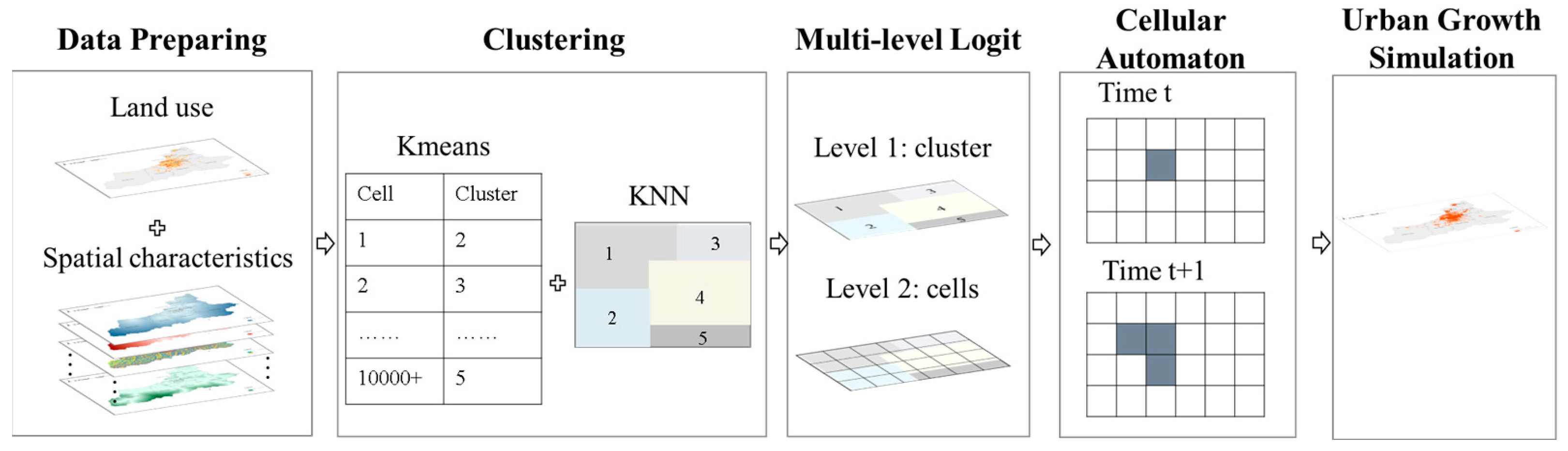
Urban growth boundaries refers to the manual demarcation lines between urban and rural areas [15]. It has been one of the most effective urban growth management tools since it was first adopted in Kentucky in 1958 [16]. UGB is now widely used in the U.S., U.K., Australia, Japan, Saudi Arabia, Iran, and Korea [17,18,19,20,21]. There is growing literature showing scholars employed the cellular automaton (CA) approach to understand the land use change. The CA approach has become one of the most popular models for simulating urban growth due to its simplicity and effectiveness [22,23], such as logit-CA model [24], artificial neural networks (ANN) CA [25], FLUS [26], and SLEUTH [27,28]. In general, the constrained cellular automaton model involves an array of cells with different temporary states and calculates cell state transition rules while incorporating previous state and neighborhood effects. When used to simulate land-use change, CA models predict land-use state based on the analysis of historical urban land-use dynamics and relevant driving factors [29], including topography, such as slope and river [30,31,32]; socio-economic factors, such as population and GDP [26,33]; transportation facilities, including roads, railways, stations, and airports [30,32,34]; urban functions, such as distance to city center [30,32] and climate [26].

China has the fastest processes of urban development in the world; land urbanization is twice as fast compared to population urbanization [35]. In this sense, China’s new spatial planning emphasizes a top-down coordination and transmission for the goal of environment sustainable. Thus, the idea of bottom-up aggregating the urban growth boundaries of each city and town based on the traditional CA model needs to be revised. It is intuitively believed the CA model could be challenged since the hierarchical relationship and development type inherent in the towns will cause the space not to develop uniformly. The scholars endeavored to echo the complexity and uncertainty of urban situations, for instance, Ke and Qi [36] used a clustering algorithm to divide Wuhan into multiple subregions and then used a decision tree to develop land conversion rules for different subregions. Shu and Bakker [37] proposed the variable weights LCA (VW-LCA) model to simulate the dynamic urban growth boundary by incorporating spatial–temporal heterogeneity into the traditional logistic CA (LCA). Liang and Liu [38] used fuzzy clustering to detect potential urban growth start zones and urban expansion rules in economic development zones.

Motivated by this trigger, we propose a CM-CA urban growth simulation model to control the spatial heterogeneity and homogeneity of the urban growth pattern. Previous literature classifies urban growth patterns from three perspectives. The first are morphologic characteristics, such as spatial patterns and landscape characteristics [39,40]. Salvati and Carlucci [14] found the urban form and landscape characteristics of city level can reflect European cities’ local socioeconomic context and urbanization trends. Different spatial structures may also lead to various land demands and affect UGB delineation [21]. Sun and Wu [41] and Liu and Ma [42] quantified different types of urban growth as infilling growth, outlying growth, or edge-expanding growth. Second is the driving mechanisms perspective. The natural environment, transportation accessibility, policy, and socioeconomic status are commonly seen as urban-growth-driving factors [43,44,45,46,47,48]. All social, economic, and physical constituents of urban growth lead to spatial–temporal changes [4,49]. For example, Shu and Zhang [50] found port-proximity-led growth or road-proximity-led growth types in three towns in China. The study also highlighted the driving mechanism varies by region and phase. Tombolini and Zambon [49] found even among cities with similar territorial characters, their unique socio-spatial and economic structure led to urban growth occurring in different ways. Third are the urbanization process characteristics, such as population density [51], land-use type [52], and urban growth rate [53]. Notably, the same urban growth type may share more common land-use change mechanisms.

The third law of geography indicates two points (areas) with more similarities in geographic configurations have more similarities in the values of target variables [54]. In this vein, taking the whole municipal as a single study area may overlook the spatial heterogeneity within cities, even if the study is conducted on a small administrative unit, such as a town [50]. Thus, we believe the CM-CA urban growth could fit the goal of China’s territory spatial planning, highlighting the differences among urban growth types in a coordinated, controllable, and supervised manner. By taking Xi’an as example, we hypothesized that firstly, multi urban growth types exist within the municipal area and may mismatch with sub-administrative boundary. Secondly, the urban growth rules show differences among urban growth types, while showing similarities within the same types.

3. Method Design

In this study, we proposed a CM-CA-based urban growth simulation method, including clustering (C), the multilevel logit model (M), and the cellular automaton (CA) model (Figure 1). (1) Clustering: K-means clustering and the K-nearest neighbors (KNN) algorithm were used to divide all land cells, which were set as 30-m resolution, in the study area into several clusters. K-means clustering enables the division of multi-dimensional data into clusters by defining prototypes and calculating the distance to each prototype [55], while KNN can further determine the attribute features of a spatially neighboring sample [36,56,57]. In our study, we highlighted differences in local spatial and socio-economical characteristics. We hypothesized land cells with the same characteristics share more common land conversion rules. The land cells, which were non-urban land at the moment t₁ and urban land at the moment t₂, were selected and clustered by K-means clustering based on their spatial and socio-economical characteristics. Then, the KNN algorithm further clusters all land cells based on K-means cluster results and spatial neighbors.

$${\arg }_s\min {\displaystyle \sum }_{i=1}^k{\displaystyle \sum }_{a\in S_i}{\left|\left|a-{\mu }_i\right|\right|}^2={\arg }_{\mathrm{s}}\min {\displaystyle \sum }_{i=1}^k\left|S_i\right|{\mathrm{VarS}}_i$$

(1)

$${\arg }_s\max \left(\mathrm{b},S_i\right)={\displaystyle \sum }_{a_j\in K}\mathrm{sim}\left(b,a_j\right)k\left(a_j,S_i\right)$$

(2)

In Formulas (1) and (2), $k$ is the number of clusters. $S_i$ is the ith cluster. ${\mu }_i$ is the average distance of the center point of ith cluster. ${\arg }_s\min$ is the set of s and a when the formula obtains its minimum value. ${\mathrm{VarS}}_i$ is the variance of $S_i$. $a_j$ is the jth of $S_i$. K is the set of nearest neighbors of $a_j. {\arg }_s\max$ is the set of s and b when the formula gets its maximum value. $\mathrm{sim}\left(b,a_j\right)$ is the similarity test of $b$ and $a_j$. $k\left(a_j,S_i\right)$ involves 0 (when $a_j$ does not belongs to $S_i$) or 1 (when $a_j$ belongs to $S_i$).

(2) Multilevel logit model: The multilevel logit model was used to calculate the influence weights of each spatial and socio-economical driving factors with both land cells and cluster levels. The multilevel logit model has been proven to deal with the inter-level variability in the drivers of urban expansion at different spatial levels [58].

$$\mathrm{Logit}\left(P_{Mlogit}\right)=\ln \left(\mathrm{odds}\right)=\ln \left(\frac{P_{Mlogit}}{1-P_{Mlogit}}\right)={\beta }_0+{\beta }_1{x}_1+\cdots +{\beta }_n{x}_n+{\alpha }_{Si}$$

(3)

In Formula (3), $P_{Mlogit}$ is the land-use change status, while 1 is for non-urban to urban land and 0 for unchanged. X is the driving factor. ${\alpha }_{Si}$ is the effects of cluster $S_i$.

(3) Cellular automaton model: The land development potential and development restriction area raster were put into the self-adopted CA model. Land demand was calculated by Markov chains, which are widely used in town expansion simulation forecasting [59,60].

3.1. Study Area

Rapid urban growth in China has gradually shifted from the southeastern coast to the inland regions [61]. Xi’an is the capital of Shaanxi Province, China located between 107°40′ and 109°49′ E and 33°42′ and 34°45′ N (Figure 2). Xi’an has 11 districts (Xincheng, Beilin, Lianhu, Baqiao, Weiyang, Yanta, Yanliang, Lintong, Changan, Gaoling, and Huyi), two counties (Lantian and Zhouzhi), and a custody national-level district (Xixian New Area). The jurisdiction is 204 km long from east to west and 116 km wide from north to south. The Qinling mountainous area and Weihe Plain make up the landforms of Xi’an. Most of the built-up areas are located in Weihe Plain. Xi’an has a history of over 3100 years. The total area is 10,108 square kilometers of which the urban area is 3582 square kilometers. The total population was 12.87 million in 2021, and 79.49% were urban residents.

3.2. Data Source

The data source of land-use types was the GlobeLand30, global land-use remote sensing data released by the Ministry of Natural Resources of China in 2010 and 2020 at 30-m resolution (Jun et al., 2014). The land cover types in Xi’an include cropland, forest land, grassland, wetland, water bodies, and artificial surfaces. In addition, the built-up area boundary was extracted from the 2010 and 2018 national built-up area boundary data released by Li et al. (2020). In this paper, the artificial surface within the built-up area boundary was considered urban land, and the other was non-urban land (Figure 3).

In this paper, the driving factors for urban growth were selected based on previous studies [26,30,31,32,33,34], including five aspects: natural topography, transportation facilities proximity, urban facilities proximity, urban structure, and economic factors. Natural topography involves slope and related aspects. Transportation facilities proximity involves distance to the train station, distance to the coach station, distance to the airport, distance to the subway station, distance to city road, distance to the railroad, and distance to the highway. Urban facilities proximity involves distance to colleges and universities, distance to shopping centers, distance to companies, and distance to hospitals. The urban structure involves distance to local government agencies and the city’s geometric center. Finally, economic factors involve GDP per square kilometer.

The restricted areas in this study include unsuitable areas for urban construction and river and cultural relic protection units at the provincial and national levels in Xi’an. Unsuitable areas for urban construction were set according to China’s dual environmental evaluation (DEE), including areas with a shortage of water resources, excessive slope of the terrain, high altitude, and extremely high risk of geological disasters. DEE has significant meanings on balancing China’s urbanization and its natural resource depletion [56]. All factors are processed at a 30-m resolution in ARC GIS 10.7 (

Table 1. Data source of land-use and driving factors.

Type	Data	Units	Year	Data Source and Processing
Land use	Land-use cover	/	2010,2020	Data from GlobeLand30. 1 for urban area and 0 for non-urban area
Natural topography	Slope	Degree	2020	Data from digital elevation model provided by Geospatial Data Cloud (https://www.gscloud.cn/home) (accessed on 1 July 2022)
	Aspect	/	2020
Transportation facilities proximity	Distance to train station	m	2020	Data from 1: 1,000,000 public version of basic geographic information data provided by National Catalogue Service for Geographic Information (https://www.webmap.cn) (accessed on 1 July 2022) Proximity was calculated by Euclidean distance in ARC GIS 10.7.
	Distance to coach station	m	2020
	Distance to airport	m	2020
	Distance to subway station	m	2020
	Distance to city road	m	2020
	Distance to railroad	m	2020
	Distance to highway	m	2020
Urban facilities proximity	Distance to colleges and universities	m	2020	Data from Gaode Open Platform (https://lbs.amap.com/) (accessed on 1 July 2022) Proximity was calculated by Euclidean distance in ARC GIS 10.7.
	Distance to shopping centers	m	2020
	Distance to companies	m	2020
	Distance to hospitals	m	2020
Urban structure	Distance to local government agencies	m	2020	Data from Gaode Open Platform (https://lbs.amap.com/) (accessed on 1 July 2022) Proximity was calculated by Euclidean distance in ARC GIS 10.7.
	Distance to center	m	2020
Economic factors	GDP per square kilometers	Yuan/km2	2010	Data from China GDP spatial distribution km grid dataset [62].
Restricted factors	Water resources	/	2019	Statistical Bulletin of Water Resources of Xi’an
	Altitude	m	2020	Data from Digital Elevation Model provided by Geospatial Data Cloud (https://www.gscloud.cn/home) (accessed on 1 July 2022)
	Geological disasters	/	2016	National Geological Disaster Prevention and Control 13th Five-Year Plan
	Cultural relic protection units at provincial and national level	/	2020	Xi’an Historical and Cultural City Protection Plan (2019–2035)

).

4. Results

4.1. Classification Results

K-means and KNN cluster algorithms were used to divide all land cells into nine clusters using python (Figure 4,

Table 2. The mean values of every cluster’s characteristics.

Cluster	OT	DZ	NIS	SIS	EIS	WS	NS	WOS	EOS
	Mean	Mean	Mean	Mean	Mean	Mean	Mean	Mean	Mean
Land changed	88.88%	63.81%	39.88%	9.98%	3.55%	0.87%	4.61%	0.03%	0.34%
Urban land in2010	86.55%	48.44%	56.91%	17.96%	12.09%	3.28%	11.93%	0.55%	1.67%
Urban land in2020|	97.85%	79.33%	70.84%	25.18%	14.24%	3.85%	15.21%	0.55%	1.92%
Slope	2.73	2.30	2.26	4.77	11.57	19.90	3.61	24.63	15.26
Aspect	184.28	187.15	176.46	181.38	186.48	178.56	174.97	175.24	182.40
Distance to train station	5319.51	8031.08	5530.86	15,705.85	9404.12	38,932.66	13,048.35	84,873.23	25,926.89
Distance to airport	27,504.24	29,604.12	18,865.97	36,544.54	47,386.43	52,152.24	32,497.70	82,795.05	67,345.78
Distance to subway station	769.90	1627.12	2640.03	7291.27	12,410.54	27,682.97	13,034.84	70,899.99	31,884.62
Distance to city road	750.77	1027.00	1581.17	1496.43	2816.20	5069.36	1191.93	7110.39	2756.58
Distance to railroad	3659.30	4519.74	1388.41	5479.90	4548.82	6949.57	6515.03	32,832.64	12,460.07
Distance to highway	2877.12	1364.51	1546.70	2764.84	6025.00	7146.71	2878.98	37,231.72	6051.43
Distance to colleges and university	774.66	1440.38	2110.46	4421.63	8065.32	9599.70	4599.22	29,290.74	14,530.31
Distance to shopping center	312.08	596.94	838.47	1502.10	3248.28	5073.79	1740.99	15,344.59	4823.38
Distance to companies	121.58	215.42	242.14	696.26	2028.99	2718.09	768.44	7938.00	3053.74
Distance to hospitals	690.36	1515.61	1692.65	3958.42	5792.40	11,617.91	2793.98	22,339.42	10,431.43
Distance to local government agencies	727.78	1963.91	2025.63	4269.77	9618.54	15,679.66	5169.62	31,663.20	27,395.15
Distance to center	20,022.64	16,849.66	28,103.68	13,810.31	36,005.25	23,043.75	51,379.60	66,180.72	63,614.50
GDP per square kilometers	157,019.10	77,716.75	32,388.96	6681.43	78,704.52	100,156.80	37,986.21	237,074.90	253,584.40

). Xi’an now has 11 districts, two counties, and one custody national-level district. Among all 11 districts, six districts in downtown, including Beilin, Yanta, Weiyang, Lianhu, Baqiao, and Xincheng, are regarded as the main city area and have high similarities. In this vein, the number of clusters was set to nine, including old town (OT), developed zone (DZ), northern inner suburb (NIS), southern inner suburb (SIS), eastern inner suburb (EIS), western suburb (WS), northern suburb (NS), western outer suburb (WOS), and eastern outer suburb (EOS). The cluster results show a ring structure around downtown and correlations with the county and district administrative boundaries.

Old Town includes the Lianhu district, Beilin district, Yanta district, and Xincheng district having the highest proportions of urbanization areas. In 2020, the land area was 97.85% compared to 86.55% in 2010. OT also has the highest rate of increase in urban land. From 2010 to 2020, 88.88% of non-urban land was transferred to urban land. The developed zone has the smallest area, only accounting for 0.47% of the whole city. DZ is mainly distributed around the Xi’an bypass highway in the Yanta district, and most areas are in Xi’an Hi-tech Industries Development Zone and Qujiang New Zone. Northern inner suburb is mainly located in the Weiyang district, which is one of the six districts in the main city. NIS has the shortest average distance to the railway. Southern inner suburb is located in the northern part of the Changan district, which is close to downtown. Eastern inner suburb distributes among the east from the downtown involving the Baqiao district, the southeast part of the Changan district, and the west part of Lantian County and the Lintong district. This cluster mainly comprises the east suburbs of the city. Western suburb is mainly located in the Huyi district and the southwest part of the Changan district. The Huyi district was established in 2017, formerly known as Hu County. The south of the Huyi district and southwest of the Changan district are the Qinling Mountains. Northern suburb is located in the Gaoling district, north of the Baqiao district, and northwest of the Lintong district. The Gaoling district, which used to be Gaoling County before 2015, is one of the longest historical counties in China. Both the Baqiao district and the Lintong district have long lengths from north to south, which may lead to the result that towns adjacent to Gaoling district are in NS. Western outer suburb is mainly distributed in Zhouzhi County. Eastern outer suburb is the eastern part of Xi’an, including the Yanliang district, the Lintong district, and Lantian County. All these districts or counties are far from downtown.

4.2. Multilevel Logit Model

A multilevel logit model was used to explore the probability of land use changing. Firstly, the multicollinearity of all the factors was examined by a variance inflation factor (VIF) with the rule that VIF < 5 and mean VIF < 3. Then, the driving factors were standardized and put into the multilevel logit model in STATA 17. After sampling 5% of land cells with changed and unchanged land use properties, the model results are shown in

Table 3. Results of multi-level logit model.

	Coefficient	Standard Error	95% Confidence Interval
Fixed effects
Slope	−0.62 ***	0.07	−0.76	−0.48
Aspect	0.00	0.01	−0.03	0.02
Distance to train station	−2.41 ***	0.08	−2.57	−2.24
Distance to city road	0.03	0.06	−0.09	0.14
Distance to railroad	0.39 ***	0.06	0.28	0.50
Distance to companies	−19.69 ***	0.30	−20.28	−19.10
Distance to local government agencies	−2.34 ***	0.08	−2.49	−2.18
Distance to center	−1.09 ***	0.05	−1.19	−1.00
GDP per square kilometers	1288.66 ***	57.01	1176.93	1400.40
constant	−9.60 ***	0.88	−11.33	−7.88
Random effects	Estimate	standard error	95% confidence interval
var(constant)	3.94	1.91	1.52	10.19

*** p < 0.001.

. We first set a null model with no independent variables to test the effects of the different clusters on land-use change. The intraclass correlation (ICC) was 73.75%, indicating the powerful effects of clusters. Table 3 showed economic factors, such as GDP and distance to companies, played the most important role in Xi’an’s urban growth. Almost half of China’s observed urban land expansion was fostered by GDP [44]. Additionally, transportation proximity and urban structure also played crucial roles in driving land-use change. The results showed lower slope, shorter distance to transportation, and shorter distance to city geometric or district political center positively affected the urban growth in Xi’an, except the land cells near the railroad had lower urban growth potential. One explanation may be that, unlike train stations, the railroad is a through-traffic and may reduce the land value.

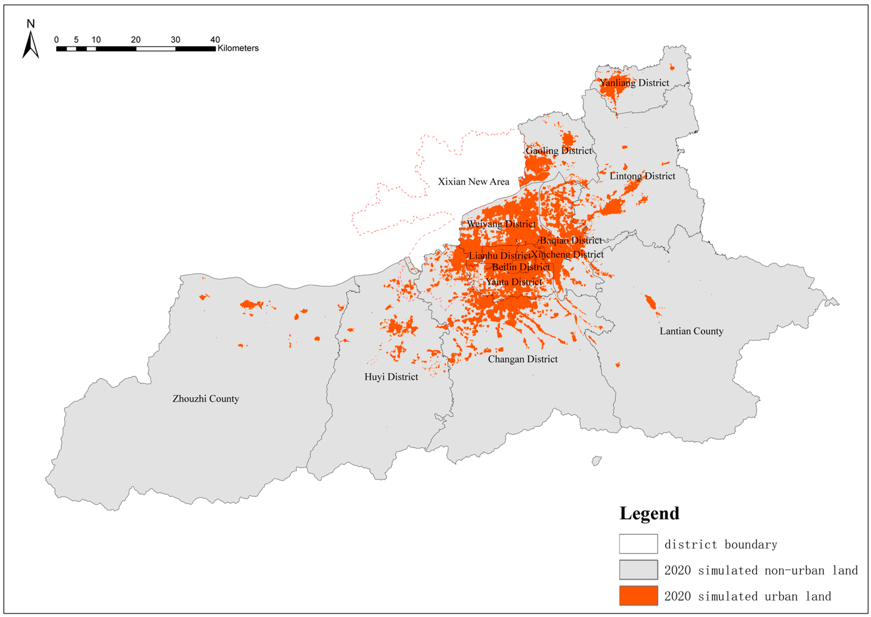
4.3. Urban Growth Simulation in Xi’an

The land-use demand in 2030 was calculated through the Markov Chain, which is widely used in the simulation of urban growth [59,60]. According to GlobeLand30, between 2010 and 2020, the urban area in Xi’an increased from 749.0 km² to 924.8 km². As calculated by the Markov Chain, the urban area in Xi’an would be 1087 km² in 2030. Self-adaptive cellular automaton was used to simulate the urban growth in Xi’an by using FLUS (Figure 5 and Figure 6). The Kappa is 0.84, and the overall accuracy is 97.28%. The overall accuracy of every cluster varied from 84.07% to 99.94%, except DZ (64.16%). In our results (

Table 4. Comparison of CM-CA results and real land-use areas.

	2020 Land Use			2020 CM-CA	2010–2020 CM-CA	2020–2030 CM-CA
Cluster	Non-Urban Area (km2)	Urban Area (km2)	Urban Area Percentage	Urban Area Percentage	Urban Growth Rate	Urban Growth Rate
OT	345.42	15,657.39	97.84%	86.22%	−0.0033	−0.0004
DZ	990.63	3810.6	79.37%	47.11%	−0.0132	−0.0051
NIS	8397.45	20,377.44	70.82%	70.35%	0.1344	0.0681
EIS	95,548.77	15,870.42	14.24%	16.86%	0.0477	0.0505
SIS	49,361.22	16,629.84	25.20%	25.60%	0.0764	0.0718
NS	38,716.65	6943.59	15.21%	16.35%	0.0442	0.0493
WS	158,312.7	6348.06	3.86%	3.69%	0.0041	0.0057
WOS	302,944.7	1666.89	0.55%	0.53%	−0.0002	−0.0002
EOS	263,164.5	5161.5	1.92%	1.97%	0.0031	0.0031

), the urban growth rate of DZ from 2010 to 2020 was −0.01, and its proportion of urban areas was only 47.11% in 2020. However, the proportion of the urban area reached 79.37% in 2020. DZ is mainly distributed in the development zone of Xi’an. In this vein, urban growth may not only follow its developmental pattern but is also strongly affected by government policy.

Table 4 shows the comparison simulation results for CM-CA and Xi’an actual land cover in 2020, including non-urban area, urban area, urban area percentage, and also the predicted urban growth rates from 2010 to 2020 and 2020 to 2030 by CM-CA. CM-CA simulation results showed the highest similarity with the actual land cover in cluster NIS, WS, WOS, EOS, and SIS. The error was less than one percent. However, the urban area percentage of OT and DZ simulated by CM-CA was lower, while those of EIS and NS were higher. CM-CA indicated less urban growth in downtown but more in the eastern urban periphery. As for the predicted urban growth rate, Table 4 shows that SIS, NIS, EIS, and NS have the highest urban growth rates from 2020 to 2030, mostly located in the inner suburb. WS and EOS are in the second-tier growth rate. As for OT, DZ, and WOS, the results showed the urban area would decrease from 2020 to 2030. Both OT and DZ were in downtown and had few non-urban lands to be developed. WOS is located in Zhouzhi County. It is nearly 70 km from Zhouzhi to downtown, which may cause the slow growth of WOS. Additionally, DZ and WOS have lower urban development potential due to their natural accessibility conditions. Xi’an City Master Plan (2008–2020) highlights the ecological functions of the Zhouzhi wetland nature reserve.

5. Discussion

In this study, we took Xi’an, the capital of the inland province, as an example and tried to delineate UGB using CM-CA. Firstly, we classified nine urban growth types and then used multi-level logit models to find the effects of driving factors on every group. The urban growth types explained over 70% of the land-use change variances, indicating urban growth type played a more important role in transferring non-urban areas into urban areas than the characteristics of the land itself.

The results were in line with our hypotheses. The urban growth types and subregion administrative boundaries were a mismatch. Urban growth mechanisms varied among different urban growth types and affected the accuracy of urban grow simulations as results. Our results found the urban growth types had higher correlations with administrative boundaries in downtown and remote suburban areas but lower correlations in the urban periphery. The urban growth development potential is based on geometric proximity rather than administrative level. The urban periphery is more likely to contain heterogeneous urban growth types than downtown or remote suburban areas. The urban growth in the urban periphery is driven by both district level and city level factors. In this vein, geometric proximity and administrative boundary show dual effects on forming urban growth types.

The simulation results show a circle structure of urban growth as the inner areas grow smoothly. The urban periphery grows rapidly, while remote suburbs of the city decay. Xi’an is a monocentric city with the Yanta, Lianhu, Belin, and Xincheng districts accounting for 50% of GDP from less than 5% of its areas. The production factor agglomeration makes the core of the city or remote suburban area growth rely on individual driving factors. With the shortage of non-urban areas in downtown, more land development potential would transfer to the urban periphery and may cause urban sprawl. In the next stage, Xi’an prepared to build Xi’an Great Ring Highway, which would reduce the traffic time from remote suburbs to downtown. As a result, the land development potential in remote suburbs and land along the road may foster a more balanced urban growth. To optimize city and town spatial layout, Xi’an should carefully make a land-use plan in the decaying clusters and guide urban growth in ecologically friendly ways. Our study is in line with previous studies that found using uniform rules to simulate urban growth may have limitations because of the varying driving factors of different urban expansion types [42].

As for the driving factors of urban growth, compared to the land cell level’s effects, urban growth types played a prominent role. Thus, the land-use policy can consider the urban growth types. On the other hand, economic factors play the most important roles at the land cell level, especially GDP. Previous studies suggested not only does economic growth foster urban growth, but also urban growth leads to economic growth [63]. In this vein, for the rapid urbanization of cities, the urban growth boundary delineation needs to cooperate with economic and industrial planning for smart growth to balance the spatial integration under compact city planning and market-driven spatial allocation.

Political effects, such as administrative zoning adjustment and new development zoning, also affect the urban growth types and development potential. Liu and Zhang [64] indicate the land-use strategy and regional development are the main forces of China’s land-use change. Shaobo and Xiaolong [65] also highlight the government’s power in urban expansion. The previous studies explored the urban growth rates under different land-use policies [66]. In our study, we found the simulation model had unsatisfactory accuracy on DZ, which is mainly located in special policy zones. Cellular automaton, as other land-use change simulation models, has limitations on coping with planning or policy effects. Recently, a number of studies have tried to consider the planning or policy in urban simulation models, such as seeing planning or policy as driving factors [60] or changing land demand of specific areas [67]. More research is needed to explore the planning strategies’ effects on future urban growth.

6. Conclusions

Under the background of China Territorial Spatial Planning, this paper tried to solve the challenge of coordinating all county and district UGBs within a municipal area by putting forward a CM-CA model. Our results found urban growth of districts and counties are influenced by multi-level factors. The urban growth types have even stronger effects than land cell level factors. The mismatch between urban growth types and district or county administrative boundaries indicates the linkages between sub-regions are increasingly based on geographic proximity and the urban flows, while the influence of administrative divisions is gradually diminishing. Delineating UGB based solely on the districts and counties themselves may overlook the higher-level influences, such as inter-regional linkages. Thus, municipal level UGB should not be a simple aggregation of subordinate district or town UGBs.

In this paper, we integrate hierarchy into the CA model with the aim of optimizing the allocation of land resources and considering local urban growth mechanisms at the same time. The urban growth of the United States and other countries is mainly due to population growth, the popularity of automobiles, and the low cost of newly developed land. The U.S. has market demand-led expansion, while the urban growth in China relies more on the agglomeration of industrial capital and urbanization brought by the pursuit of economic growth of local governments and is more like a government supply-led growth [68]. In China, the municipal government plays an important role in resource relocation and directly affects urban growth by assigning future urban construction land indicators of districts and counties. The land space development rights and relevant policies are tightly linked to administrative hierarchy. In our example, we distinguish urban growth types based on land cell characteristics. Xi’an is a prefecture-level city with districts and counties. Eight of the nine urban growth types are mainly distributed among districts, and the other was in Zhouzhi County. Even though Zhouzhi and Lantian are in the same administrative level as county, Lantian County is much closer to the city center and shared the same types with the nearby districts of Lintong and Yanliang.

We assume the same hierarchy structure of urban growth may also happen in other regions, such as metropolitan areas. Delineating UGB solely without cooperation between administrative units would lead to ineffective competition, urban expansion, and waste of resources. Therefore, the local authority calls for urban growth rather than smart growth.

References

1. United Nations. World Urbanization Prospects: The 2018 Revision; United Nations: New York, NY, USA, 2018. [Google Scholar]
2. Seto Karen, C.; Güneralp, B.; Lucy, R.H. Global forecasts of urban expansion to 2030 and direct impacts on biodiversity and carbon pools. Proc. Natl. Acad. Sci. USA 2012, 109, 16083–16088. [Google Scholar] [CrossRef] [PubMed] [Green Version]
3. Angel, S.; Parent, J.; Civco, D.L.; Blei, A.; Potere, D. The dimensions of global urban expansion: Estimates and projections for all countries, 2000–2050. Prog. Plan. 2011, 75, 53–107. [Google Scholar] [CrossRef]
4. Aldalbahi, M.; Walker, G. Attitudes and policy implications of urban growth boundary and traffic congestion reduction in Riyadh, Saudi Arabia. In Proceedings of the International Conference Data Mining, Atlantic City, NJ, USA, 14–17 November 2015. [Google Scholar]
5. McDonald, R.I.; Green, P.; Balk, D.; Fekete, B.M.; Revenga, C.; Todd, M.; Montgomery, M. Urban growth, climate change, and freshwater availability. Proc. Natl. Acad. Sci. USA 2011, 108, 6312–6317. [Google Scholar] [CrossRef] [PubMed] [Green Version]
6. Dinka, M.O.; Klik, A. Effect of land use–land cover change on the regimes of surface runoff—The case of Lake Basaka catchment (Ethiopia). Environ. Monit. Assess. 2019, 191, 278. [Google Scholar] [CrossRef] [PubMed]
7. Guzha, A.C.; Rufino, M.; Okoth, S.; Jacobs, S.; Nóbrega, R. Impacts of land use and land cover change on surface runoff, discharge and low flows: Evidence from East Africa. J. Hydrol. Reg. Stud. 2018, 15, 49–67. [Google Scholar] [CrossRef]
8. Ewing, R.; Lyons, T.; Siddiq, F.; Sabouri, S.; Kiani, F.; Hamidi, S.; Choi, D.-A.; Ameli, H. Growth Management Effectiveness: A Literature Review. J. Plan. Lit. 2022, 37, 08854122221077457. [Google Scholar] [CrossRef]
9. Wang, Z.; Wu, F. Regional and urban planning for growth in China. In International Encyclopedia of Geography: People, the Earth, Environment and Technology; John Wiley and Sons Ltd.: Hoboken, NJ, USA, 2020; pp. 1–8. [Google Scholar]
10. American Planning Association. Growing Smart Guidebook. Chapter 6—Regional Planning; American Planning Association: Washington, DC, USA, 2002. [Google Scholar]
11. Pacione, M. Urban Geography From Global to Local. In Urban Geography: A Global Perspective; Routledge: London, UK, 2009; pp. 1–15. [Google Scholar]
12. Strano, E.; Viana, M.; da Fontoura Costa, L.; Cardillo, A.; Porta, S.; Latora, V. Urban Street Networks, a Comparative Analysis of Ten European Cities. Environ. Plan. B Plan. Des. 2013, 40, 1071–1086. [Google Scholar] [CrossRef] [Green Version]
13. Dibble, J.; Prelorendjos, A.; Romice, O.; Zanella, M.; Strano, E.; Pagel, M.; Porta, S. On the origin of spaces: Morphometric foundations of urban form evolution. Environ. Plan. B Urban Anal. City Sci. 2017, 46, 707–730. [Google Scholar] [CrossRef] [Green Version]
14. Salvati, L.; Carlucci, M. Land-use structure, urban growth, and periurban landscape: A multivariate classification of the European cities. Environ. Plan. B Plan. Des. 2015, 42, 801–829. [Google Scholar] [CrossRef]
15. Nelson, A.C.; Moore, T. Assessing urban growth management: The case of Portland, Oregon, the USA’s largest urban growth boundary. Land Use Policy 1993, 10, 293–302. [Google Scholar] [CrossRef]
16. Nelson, A.C.; Duncan, J.A.B. Growth Management Principles and Practices; Planners Press: Chicago, IL, USA, 1995. [Google Scholar]
17. Tayyebi, A.; Pijanowski, B.C.; Tayyebi, A.H. An urban growth boundary model using neural networks, GIS and radial parameterization: An application to Tehran, Iran. Landsc. Urban Plan. 2011, 100, 35–44. [Google Scholar] [CrossRef]
18. Mubarak, F.A. Urban growth boundary policy and residential suburbanization: Riyadh, Saudi Arabia. Habitat Int. 2004, 28, 567–591. [Google Scholar] [CrossRef]
19. Ding, C.; Knaap, G.J.; Hopkins, L.D. Managing urban growth with urban growth boundaries: A theoretical analysis. J. Urban Econ. 1999, 46, 53–68. [Google Scholar] [CrossRef]
20. Venkataraman, M. Analyzing Urban Growth Boundary Effects in the City of Bengaluru. ERN Urban Rural. Anal. Dev. Econ. (Top.) 2014, 49, 54–61. [Google Scholar] [CrossRef]
21. Guo, Q.; Chen, X.; Zhu, Y. A Study on Urban Growth Boundary Delimitation: The Case of Baoji, Weinan and Ankang Urban Master Plan. Open Cybern. Syst. J. 2015, 9, 1710–1715. [Google Scholar]
22. Santé, I.; García, A.M.; Miranda, D.; Crecente, R. Cellular automata models for the simulation of real-world urban processes: A review and analysis. Landsc. Urban Plan. 2010, 96, 108–122. [Google Scholar] [CrossRef]
23. Liu, X.; Li, X.; Shi, X.; Zhang, X.; Chen, Y. Simulating land-use dynamics under planning policies by integrating artificial immune systems with cellular automata. Int. J. Geogr. Inf. Sci. 2010, 24, 783–802. [Google Scholar] [CrossRef]
24. Cheng, J.; Masser, I. Understanding spatial and temporal processes of urban growth: Cellular automata modelling. Environ. Plan. B Plan. Des. 2004, 31, 167–194. [Google Scholar] [CrossRef]
25. Yang, X.; Chen, R.; Zheng, X.Q. Simulating land use change by integrating ANN-CA model and landscape pattern indices. Geomat. Nat. Hazards Risk 2016, 7, 918–932. [Google Scholar] [CrossRef] [Green Version]
26. Liu, X.; Liang, X.; Li, X.; Xu, X.; Ou, J.; Chen, Y.; Li, S.; Wang, S.; Pei, F. A future land use simulation model (FLUS) for simulating multiple land use scenarios by coupling human and natural effects. Landsc. Urban Plan. 2017, 168, 94–116. [Google Scholar] [CrossRef]
27. Silva, E.A.; Clarke, K.C. Calibration of the SLEUTH urban growth model for Lisbon and Porto, Portugal. Comput. Environ. Urban Syst. 2002, 26, 525–552. [Google Scholar] [CrossRef]
28. Osman, T.; Divigalpitiya, P.; Arima, T. Using the SLEUTH urban growth model to simulate the impacts of future policy scenarios on land use in the Giza Governorate, Greater Cairo Metropolitan region. Int. J. Urban Sci. 2016, 20, 407–426. [Google Scholar] [CrossRef]
29. Li, X.; Yeh, A.G.-O. Neural-network-based cellular automata for simulating multiple land use changes using GIS. Int. J. Geogr. Inf. Sci. 2002, 16, 323–343. [Google Scholar] [CrossRef]
30. Liu, Y.; He, Q.; Tan, R.; Liu, Y.; Yin, C. Modeling different urban growth patterns based on the evolution of urban form: A case study from Huangpi, Central China. Appl. Geogr. 2016, 66, 109–118. [Google Scholar] [CrossRef]
31. Müller, K.; Steinmeier, C.; Küchler, M. Urban growth along motorways in Switzerland. Landsc. Urban Plan. 2010, 98, 3–12. [Google Scholar] [CrossRef]
32. He, Q.; Tan, R.; Gao, Y.; Zhang, M.; Xie, P.; Liu, Y. Modeling urban growth boundary based on the evaluation of the extension potential: A case study of Wuhan city in China. Habitat Int. 2018, 72, 57–65. [Google Scholar] [CrossRef]
33. Wu, K.-Y.; Zhang, H. Land use dynamics, built-up land expansion patterns, and driving forces analysis of the fast-growing Hangzhou metropolitan area, eastern China (1978–2008). Appl. Geogr. 2012, 34, 137–145. [Google Scholar] [CrossRef]
34. Sunde, M.G.; He, H.S.; Zhou, B.; Hubbart, J.A.; Spicci, A. Imperviousness Change Analysis Tool (I-CAT) for simulating pixel-level urban growth. Landsc. Urban Plan. 2014, 124, 104–108. [Google Scholar] [CrossRef]
35. World Bank; Development Research Center of the State Council, The People’s Republic of China. China’s Urbanization and Land: A Framework for Reform; World Bank: Washington, DC, USA, 2014. [Google Scholar]
36. Ke, X.; Qi, L.; Zeng, C. A partitioned and asynchronous cellular automata model for urban growth simulation. Int. J. Geogr. Inf. Sci. 2016, 30, 637–659. [Google Scholar] [CrossRef]
37. Shu, B.; Bakker, M.M.; Zhang, H.; Li, Y.; Qin, W.; Carsjens, G.J. Modeling urban expansion by using variable weights logistic cellular automata: A case study of Nanjing, China. Int. J. Geogr. Inf. Sci. 2017, 31, 1314–1333. [Google Scholar] [CrossRef]
38. Liang, X.; Liu, X.; Chen, G.; Leng, J.; Wen, Y.; Chen, G. Coupling fuzzy clustering and cellular automata based on local maxima of development potential to model urban emergence and expansion in economic development zones. Int. J. Geogr. Inf. Sci. 2020, 34, 1930–1952. [Google Scholar] [CrossRef]
39. Sapena, M.; Fernández, L.Á.R. Identifying urban growth patterns through land-use/land-cover spatio-temporal metrics: Simulation and analysis. Int. J. Geogr. Inf. Sci. 2021, 35, 375–396. [Google Scholar] [CrossRef]
40. Aithal, B.H.; Ramachandra, T.V. Visualization of Urban Growth Pattern in Chennai Using Geoinformatics and Spatial Metrics. J. Indian Soc. Remote Sens. 2016, 44, 617–633. [Google Scholar] [CrossRef]
41. Sun, C.; Wu, Z.-F.; Lv, Z.-Q.; Yao, N.; Wei, J.-B. Quantifying different types of urban growth and the change dynamic in Guangzhou using multi-temporal remote sensing data. Int. J. Appl. Earth Obs. Geoinf. 2013, 21, 409–417. [Google Scholar] [CrossRef]
42. Liu, X.; Ma, L.; Li, X.; Ai, B.; Li, S.; He, Z. Simulating urban growth by integrating landscape expansion index (LEI) and cellular automata. Int. J. Geogr. Inf. Sci. 2014, 28, 148–163. [Google Scholar] [CrossRef]
43. Brueckner, J.K. Urban Sprawl: Diagnosis and Remedies. Int. Reg. Sci. Rev. 2000, 23, 160–171. [Google Scholar] [CrossRef]
44. Seto, K.C.; Fragkias, M.; Güneralp, B.; Reilly, M.K. A meta-analysis of global urban land expansion. PLoS ONE 2011, 6, e23777. [Google Scholar] [CrossRef] [PubMed]
45. Wang, Y.; Han, Y.; Pu, L.; Jiang, B.; Yuan, S.; Xu, Y. A Novel Model for Detecting Urban Fringe and Its Expanding Patterns: An Application in Harbin City, China. Land 2021, 10, 876. [Google Scholar] [CrossRef]
46. Nong, Y.; Du, Q. Urban growth pattern modeling using logistic regression. Geo-Spat. Inf. Sci. 2011, 14, 62–67. [Google Scholar] [CrossRef]
47. Dubovyk, O.; Sliuzas, R.; Flacke, J. Spatio-temporal modelling of informal settlement development in Sancaktepe district, Istanbul, Turkey. ISPRS J. Photogramm. Remote Sens. 2011, 66, 235–246. [Google Scholar] [CrossRef]
48. Li, X.; Zhou, W.; Ouyang, Z. Forty years of urban expansion in Beijing: What is the relative importance of physical, socioeconomic, and neighborhood factors? Appl. Geogr. 2013, 38, 1–10. [Google Scholar] [CrossRef]
49. Tombolini, I.; Zambon, I.; Ippolito, A.; Grigoriadis, S.; Serra, P.; Salvati, L. Revisiting “Southern” Sprawl: Urban Growth, Socio-Spatial Structure and the Influence of Local Economic Contexts. Economies 2015, 3, 237–259. [Google Scholar] [CrossRef] [Green Version]
50. Shu, B.; Zhang, H.; Li, Y.; Qu, Y.; Chen, L. Spatiotemporal variation analysis of driving forces of urban land spatial expansion using logistic regression: A case study of port towns in Taicang City, China. Habitat Int. 2014, 43, 181–190. [Google Scholar] [CrossRef]
51. Lu, D.; Weng, Q. Use of impervious surface in urban land-use classification. Remote Sens. Environ. 2006, 102, 146–160. [Google Scholar] [CrossRef]
52. Dadhich, P.N.; Hanaoka, S. Spatio-temporal Urban Growth Modeling of Jaipur, India. J. Urban Technol. 2011, 18, 45–65. [Google Scholar] [CrossRef]
53. Tian, G.; Jiang, J.; Yang, Z.; Zhang, Y. The urban growth, size distribution and spatio-temporal dynamic pattern of the Yangtze River Delta megalopolitan region, China. Ecol. Model. 2011, 222, 865–878. [Google Scholar] [CrossRef]
54. Zhu, A.-X.; Lu, G.; Liu, J.; Qin, C.-Z.; Zhou, C. Spatial prediction based on Third Law of Geography. Ann. GIS 2018, 24, 225–240. [Google Scholar] [CrossRef]
55. Bárcena, J.F.; Camus, P.; García, A.; Álvarez, C. Selecting model scenarios of real hydrodynamic forcings on mesotidal and macrotidal estuaries influenced by river discharges using K-means clustering. Environ. Model. Softw. 2015, 68, 70–82. [Google Scholar] [CrossRef]
56. Zhang, D.; Liu, X.; Lin, Z.; Zhang, X.; Zhang, H. The delineation of urban growth boundaries in complex ecological environment areas by using cellular automata and a dual-environmental evaluation. J. Clean. Prod. 2020, 256, 120361. [Google Scholar] [CrossRef]
57. Guo, G.; Wang, H.; Bell, D.; Bi, Y.; Greer, K. KNN Model-Based Approach in Classification. In On The Move to Meaningful Internet Systems 2003: CoopIS, DOA, and ODBASE; Springer: Berlin/Heidelberg, Germany, 2003. [Google Scholar]
58. Shu, B.; Zhu, S.; Qu, Y.; Zhang, H.; Li, X.; Carsjens, G.J. Modelling multi-regional urban growth with multilevel logistic cellular automata. Comput. Environ. Urban Syst. 2020, 80, 101457. [Google Scholar] [CrossRef]
59. Balzter, H. Markov chain models for vegetation dynamics. Ecol. Model. 2000, 126, 139–154. [Google Scholar] [CrossRef]
60. Zhou, L.; Dang, X.; Sun, Q.; Wang, S. Multi-scenario simulation of urban land change in Shanghai by random forest and CA-Markov model. Sustain. Cities Soc. 2020, 55, 102045. [Google Scholar] [CrossRef]
61. Deng, X.; Bai, X. Sustainable urbanization in western China. Environ. Sci. Policy Sustain. Dev. 2014, 56, 12–24. [Google Scholar] [CrossRef]
62. Fu, J.; Jiang, D.; Huang, Y. 1 km grid population dataset of China (2005, 2010). Acta Geogr. Sin. 2014, 69 (Suppl. S1), 41–44. [Google Scholar]
63. Bai, X.; Chen, J.; Shi, P. Landscape Urbanization and Economic Growth in China: Positive Feedbacks and Sustainability Dilemmas. Environ. Sci. Technol. 2012, 46, 132–139. [Google Scholar] [CrossRef]
64. Liu, J.; Zhang, Z.; Xu, X.; Kuang, W.; Zhou, W.; Zhang, S.; Li, R.; Yan, C.; Yu, D.; Wu, S.; et al. Spatial patterns and driving forces of land use change in China during the early 21st century. J. Geogr. Sci. 2010, 20, 483–494. [Google Scholar] [CrossRef]
65. Wang, S.; Luo, X. The evolution of government behaviors and urban expansion in Shanghai. Land Use Policy 2022, 114, 105973. [Google Scholar]
66. Huang, X.; Wang, H.; Xiao, F. Simulating urban growth affected by national and regional land use policies: Case study from Wuhan, China. Land Use Policy 2022, 112, 105850. [Google Scholar] [CrossRef]
67. Bacău, S.; Domingo, D.; Palka, G.; Pellissier, L.; Kienast, F. Integrating strategic planning intentions into land-change simulations: Designing and assessing scenarios for Bucharest. Sustain. Cities Soc. 2022, 76, 103446. [Google Scholar] [CrossRef]
68. Lin, J.; Liu, W. Demarcation of Urban Development Boundary. Beijing Plan. Rev. 2014, 6, 14–21. [Google Scholar]
Figure 1. The flowchart of CM-CA model.
Land 11 02210 g001
Figure 2. The location of Xi’an.
Land 11 02210 g002
Figure 3. Urban and non-urban land of Xi’an in 2010 and 2020.
Land 11 02210 g003
Figure 4. Results of clustering.
Land 11 02210 g004
Figure 5. Urban growth simulation in 2020.
Land 11 02210 g005
Figure 6. Urban growth simulation in 2030.
Land 11 02210 g006