
Agricultural Services: Another Way of Farmland Utilization and Its Effect on Agricultural Green Total Factor Productivity in China


College of Public Administration, Nanjing Agricultural University, Nanjing 210095, China
*
Author to whom correspondence should be addressed.
Land 2022, 11(8), 1170; https://doi.org/10.3390/land11081170
Submission received: 29 June 2022
/
Revised: 21 July 2022
/
Accepted: 22 July 2022
/
Published: 27 July 2022
(This article belongs to the Special Issue Land Use Change and Anthropogenic Disturbances: Relationships, Interactions, and Management)
Abstract
:Improving agricultural green total factor productivity (AGTFP) is an important aspect of sustainable agricultural development. Agricultural services, a new way of farmland utilization in agricultural production, solved the problem of ‘who and how to farm’ in the context of labor off-farm migration. The literature has analyzed different factors that affect AGTFP, but there is a relative dearth of research into agricultural services and AGTFP. Therefore, based on the panel data of 31 provinces from 2011 to 2020, this study firstly measured carbon emissions in agricultural production and then took it as an unexpected output to measure the AGTFP by using the global Malmquist–Luenberger (GML) productivity index. Finally, the effect of agricultural services on AGTFP and its decomposition were empirically verified. The main findings are as follows: (1) Between 2011 and 2020, agricultural carbon emissions increased from 85.63 million tons to 90.99 million tons in the first five years and decreased gradually to 78.64 million tons in 2020; the government policy significantly affects carbon emissions reduction. (2) AGTFP has been increasing for the past decade, and the average growth rate of AGTFP reached 1.016, and agricultural services promoted AGTFP growth significantly, in which technological progress was the crucial driving factor. (3) Taking the Heihe–Tengchong line as the demarcation, the improving effect of agricultural services on AGTFP in the eastern region is better than the western region.
1. Introduction
Human beings have been facing great challenges for their survival since the 1960s due to global warming, environmental pollution, resource depletion, desertification, and other ecological issues [1,2,3]. In response to environmental deterioration and to achieve sustainable development, many countries have attached importance to environmental issues and economic development. Since the Reform and Opening Up in 1978, China’s agriculture has made remarkable achievements [4]. However, it also has the problem of the excessive input of chemical fertilizer, pesticides, and agricultural plastic film [5], which are detrimental to the quality of agricultural products [6] and impose an additional burden on resources and the environment. The improvement of agricultural total factor productivity (AGTFP) is crucial to addressing these issues. Compared with the traditional total factor productivity of agriculture (TFP), AGTFP incorporates unexpected output, such as carbon emissions, which is a more accurate indicator for measuring high-quality development [7,8,9].
The implementation of the Household Responsibility System (HRS) resulted in China’s agricultural operation, characterized by a small scale of farmland and a high degree of fragmentation [10]. The fragmented distribution of farmland interferes with the efficient operation of agricultural machinery, adversely affecting agricultural production [11], which poses serious threats to food security [12,13,14]. In addition, with the rapid urbanization process, the degree of labor off-farm migration keeps increasing, resulting in a serious shortage of rural labor [15,16]. Who would engage in agricultural production? How is farmland effectively utilized? As a new way of farmland utilization in agricultural production, agricultural services can practically answer the above questions. For example, households can purchase related agricultural services, mainly including plowing, planting, pesticides spraying, harvesting, and selling agricultural products [17], to realize the substitute of labor input by machineries in agricultural production. During this process, advanced technologies and management methods have been widely adopted, and the structure of various input factors has been improved, which is conducive to the improvement of farmland utilization efficiency [14,18,19].
With the continuous development of the green economy, scholars have begun to pay attention to the measurement and the essential influencing factors of AGTFP. It is found that although there was a fluctuation in AGTFP, on the whole, it represented a continued growth trend [4,6,20,21]. In terms of influencing factors on AGTFP, scholars have studied from the perspectives of farmers’ personal characteristics, environmental regulations, adjustment of agricultural structure, and technological progress. For example, if farmers are well-educated, they will be more likely to adopt advanced technologies in agricultural production, promoting the growth of AGTFP [22]. Chen found that the constraints of environmental regulations restricted farmers’ agricultural production behavior, reducing the carbon emissions and increasing the AGTFP [21]. In addition, Liu et al. and Ge et al. proved that the agricultural structure adjustment also significantly affects AGTFP [4,23]. Agriculture has both economic and ecological functions, and the optimization of the agricultural structure is conducive to high-quality agricultural development, which could promote green agricultural production [24]. Moreover, the essential role of technological progress in the improvement of AGTFP has been widely recognized [25]. For instance, by using the spatial Durbin model and Malmquist index, Wang et al. empirically test the effect of the innovation of agricultural technology on AGTFP from 2000 to 2016 [26]. Additionally, the effect on AGTFP of crop insurance [27], land transfer marketization [28], and agricultural mechanization [29] has also been empirically verified.
The measurement and influencing factors of AGTFP have been extensively examined in previous studies, but few of them have focused on the relationship between agricultural services and AGTFP. This study aims to fill this gap by mainly exploring the effect of agricultural services on AGTFP from the perspective of carbon emission. In this paper, we use panel data from 31 Chinese provinces (municipalities and autonomous regions) to calculate agricultural production carbon emissions and analyze the effect of government policies on it. Then, taking carbon emissions as unexpected output, we measure the AGTFP by using the global Malmquist–Luenberger (GML) productivity index. Finally, the effect of agricultural services on AGTFP and its decomposition is verified. In addition, taking the Heihe–Tengchong line as the demarcation, the heterogeneity analysis is conducted as well.
The study will be conducted as follows: Section 2 consists of the theoretical analysis and research hypotheses. After that, Section 3 presents the data, methodology, and empirical models. In Section 4, the results of the statistical analysis and the empirical analysis are presented. A discussion and the main conclusion are presented in Section 5 and Section 6.
2. Theoretical Analysis and Hypotheses
Economic growth was considered as a result of the division of labor [30]. The advancement of agricultural technologies has led to the continuous development of specialization and the division of labor [31,32]. The development of secondary and tertiary industries has led to a sharp increase in average salary. In order to maximize the household income, farmers are more likely to work in urban areas, which results in non-agriculture migration and a labor shortage in agricultural production. Therefore, the underutilization of farmland has been observed [33,34,35]. Agricultural machinery service is the main part of agricultural services, and the application of agricultural services can realize the substitution of labor input for machineries, which can reduce the relative cost of agricultural production. In addition, more high-tech and precise methods are introduced into agricultural production through agricultural services [36]. Therefore, the problem of farmland underutilization can be solved practically.
In agricultural production, the division of labor subdivides the relatively complex production process into independent links and promotes the invention and application of agricultural machinery [37]. However, agricultural machinery has strong asset specificity and a large sunk cost effect [38]; therefore, it is a rational choice for farmers to obtain agricultural services to replace the purchase of agricultural machinery in agricultural production. To a certain extent, agricultural services can play the role of ‘transmitter’, introducing advanced technology, a management concept, and human capital into agricultural production [39] and driving the improvement of agricultural efficiency [40,41,42,43].
In order to maximize the benefits, farmers usually overuse agrochemicals, such as pesticides, fertilizers, and plastic films, in agricultural production to increase the agricultural yield [41,42,43,44,45,46], which is harmful to natural resources and the environment [47,48]. However, in the process of agricultural services provision, the progress of agricultural technology introduces advanced green technology into agricultural production, such as the application of soil testing and formula fertilization, drip irrigation and sprinkler irrigation, and straw returning, which is conducive to reducing agrochemicals input and controlling carbon emissions in agricultural production [49]. In addition, scientific approaches allow agricultural services suppliers to utilize agrochemicals in a more precise, standardized, and reasonable way, avoiding input redundancy and reducing environmental damage [50]. It can be seen from the above analysis that agricultural services have a promoting effect on agricultural efficiency and alleviate the negative effect of agricultural production on resources and the environment, which is beneficial to sustainable agricultural development. Therefore, it is hypothesized that:
Hypothesis 1.
Agricultural services have a positive effect on AGTFP.
Agricultural green total factor productivity can be further decomposed into green technological progress and green technological efficiency [27,51]. In order to improve the efficiency and quality of agricultural services, suppliers will make full use of the present technologies at a certain technical level. The application degree of agricultural technologies and the input structure of different factors are relatively stable [52]. As a result, there is limited space to promote the improvement of AGTFP by optimizing the ratio of agricultural input and output (i.e., the improvement of technical efficiency). The increase in AGTFP is mainly attributed to green technological progress. Therefore, it is hypothesized that:
Hypothesis 2.
Green technological progress is the crucial driving factor of AGTFP.
3. Methods and Data
3.1. Calculation Method of Agricultural Carbon Emissions
Scholars conducted numerous studies on agricultural carbon emissions and its calculation method [53,54,55]. However, different studies applied various methods and provided different results. On the basis of Liu et al. [4] and IPCC [56], carbon emissions of agricultural activities are mainly summarized as follows: (1) the use of pesticides, chemical fertilizers, and agricultural films; (2) diesel consumption by agricultural machineries; (3) the damage to the soil when plowing; and (4) the use of fossil fuels in generating electricity for irrigation. The corresponding carbon emission coefficient is listed in Table 1.
Agricultural carbon emissions are calculated as follow:
where C represents agricultural carbon emissions, represents sources of agricultural carbon emissions, represents the consumption of sources, represents the carbon emission coefficient of sources.
3.2. Calculation Method of AGTFP
Using the software MaxDEA, the output-oriented distance function is applied to calculate the global Malmquist–Luenberger (GML) productivity index, which represents the AGTFP. The specific form of GML is shown in formula (2):
where , is the possible production frontier. , , represent the increase, decrease, and stability of AGTFP, respectively. Furthermore, the GML productivity index can be decomposed into two parts (as shown in formula (3)), namely agricultural green technology change (GTC) and agricultural green efficiency change (GEC).
In the process of measuring AGTFP and its decomposition, the input and output indicators are set in Table 2.
3.3. Empirical Models
According to the measurement of carbon emissions and AGTFP, formulas (4) and (5) are modeled as follows to empirically test the effect of government policy on carbon emissions and the effect of agricultural services on AGTFP and its decomposition.
In the above formulas, , represents 31 provinces (municipalities and autonomous regions), , represents different years. represents , , and , respectively. represents the logarithm of agricultural carbon emissions. is the dummy variable that represents the policy of ‘Action Plan for the zero increase of fertilizer use and pesticides by 2020’. is the core explanatory variable in formula (5), indicating the development level of agricultural services, represented by the output value of agricultural services (based on 2011) per crops planting area. In the other control variables, is the GDP per capita, representing the economic development level. is the proportion of the added value of the primary industry to GDP. is the agricultural machinery input level. is the labor input level. is a constant term, are the parameters of interest, and is the standard error. The specific information is seen in Table 2.
3.4. Data
This study uses balanced panel data of 31 provinces (municipalities and autonomous regions) in China, from 2011 to 2020, to conduct a corresponding analysis. The services output value for agriculture, forestry, animal husbandry, and fishery is from the China Statistical Yearbook of The Tertiary Industry (2012–2021). The number of agricultural employees is from 31 Provincial Statistical Yearbooks (2012–2021), and the interpolation method is used for supplementing the missing data of Liaoning Province in 2019. In addition, all other data are from China Rural Statistical Yearbook and China Statistical Yearbook (2012–2021). We exclude Hong Kong, Macau, and Taiwan from our analysis because of the inconsistent statistical caliber and some missing variables.
In the China Statistical Yearbook of The Tertiary Industry, the total services output value of agriculture, forestry, animal husbandry, and fishery is available instead of the output value of agricultural services. The output value of agricultural services is calculated as follows:
In formula (6), SA represents the output value of agricultural services; represents the output value of agriculture; represents the output value of agriculture, forestry, animal husbandry, and fishery; and represents the services output value of agriculture, forestry, animal husbandry, and fishery.
Taking the Heihe–Tengchong line as the demarcation, the east area includes 23 provincial administrative regions, Beijing, Tianjin, Hebei, Shanxi, Liaoning, Jilin, Heilongjiang, Shanghai, Jiangsu, Zhejiang, Anhui, Fujian, Jiangxi, Shandong, Henan, Hubei, Hunan, Guangdong, Guangxi, Hainan, Chongqing, Guizhou, Yunnan; the west area includes 8 provincial administrative regions, Inner Mongolia, Shaanxi, Sichuan, Tibet, Gansu, Qinghai, Ningxia, Xinjiang.
4. Results and Analysis
4.1. Results and Analysis of Carbon Emissions
As shown in Figure 1, the agricultural carbon emissions showed an inverted-‘U’ trend during the period between 2011 and 2020, with an average annual agricultural carbon emission of 86.62 million tons. It is clear that the agricultural carbon emissions kept increasing in the first half of the decade, rising from 85.63 million tons in 2011 to 90.99 million tons in 2015. In the last five years, agricultural carbon emissions showed a gradual decline trend, reducing to 78.64 million tons at the end of the decade. Compared with 2011, the agricultural carbon emissions have been reduced by 8.16% over the past ten years. From the perspective of the annual growth rate of agricultural carbon emissions, it reached the summit in 2012 (2.43%); after that, it continuously dropped to −4.130% in 2019. Although there is a slight rise in the annual growth rate of agricultural carbon emissions in 2020, it still presents a negative growth of −2.901%.
In 2015, the Chinese government implemented the policy of the ‘Action Plan for the zero increase of fertilizer use and pesticides by 2020’. All provinces responded to the call of the policy and conducted various actions, such as soil testing and formula fertilization, scientific pesticide use training, and the substitution of chemical fertilizer for green fertilizer. To verify the effect of government policy on agricultural carbon emissions, taking the logarithm of agricultural carbon emissions as the dependent variable and the policy of the ‘Action Plan for the zero increase of fertilizer use and pesticides by 2020’ as the dummy variable, we analyzed the influential effect empirically by using a fixed-effect model.
As shown in Table 3, we can see that the government policy of the ‘Action Plan for the zero increase of fertilizer use and pesticides by 2020’ has a significant negative effect on agricultural carbon emissions, indicating that the government policy controlled the total input of agrochemicals and reduced agricultural carbon emissions effectively. In addition, the estimates in column 2 show that the variables of mac and labor have a significant positive and negative effect on the agricultural carbon emissions, respectively, which makes sense because in agricultural production, machinery and labor are interchangeable. Moreover, carbon emissions from machinery are one of the main sources of carbon emissions from agriculture. However, we also found that the effects of GDP per capita and the proportion of the added value of the primary industry to GDP on agricultural carbon emissions were not significant.
4.2. Results and Analysis of AGTFP
Table 4 reports the results of the national and provincial AGTFP calculations for the years 2011 to 2020. At the national level, the AGTFP has been on an overall upward trend, except for 2015 (0.999) and 2017 (0.947), with a cumulative AGTFP growth rate of 1.068 from 2011 to 2020. Although there is a fluctuating growth trend of AGTFP in 31 provincial administrative regions, the AGTFP keeps increasing on the whole; the average growth rate reaches 1.016. The cumulative AGTFP growth rates of 31 provincial administrative regions from 2011 to 2020 are all greater than or equal to 1, except Jilin (0.923), among which Ningxia (1.548), Tianjin (1.418), and Guizhou (1.410) show the most rapid growth trend. In order to obtain more insight into the change and regional differences of AGTFP, Figure 2 provides a visualization of the results on the maps, where the darker the color, the higher the growth rate of the AGTFP is.
4.3. The Effect of Agricultural Services on AGTFP and Its Decomposition
4.3.1. Basic Regression Analysis
The fixed-effect model is applied in regression analysis, and the empirical results are shown in Table 5. The core explanatory variable, the development level of agricultural services, has a significant positive effect on AGTFP at the 5% significance level, indicating that Hypothesis 1 is confirmed. As to the other control variables, the regional development level has a significant negative effect on AGTFP at the 10% significance level. Currently, the main driving force of regional development are the secondary and tertiary industries. The higher the level of regional development, the less emphasis is placed on agriculture, which results in a decrease in AGTFP. In addition, there is a significant (1% level of significance) negative correlation between the level of labor input and AGTFP. The wide application of machinery in agricultural production has replaced a large amount of labor input in traditional agriculture and promoted the significant improvement of agricultural production efficiency. Therefore, under the background of agricultural mechanization, excessive labor input affects the comprehensive allocation efficiency between different input factors, which is not conducive to the efficiency improvement in agriculture, and then has a negative effect on AGTFP.
On this basis, further empirical tests are conducted on the decomposition of AGTFP, namely green technology change (GTC) and green efficiency change (GEC). The average growth rate of the GTC and GEC of 31 provincial administrative regions from 2011 to 2020 is 1.020 and 0.997, respectively, representing the progress of green technology and the retrogression of green efficiency. The empirical results show that agricultural services can improve GTC significantly. Although agricultural services are also conducive to the improvement of GEC, the effect is insignificant, indicating that GTC is the crucial driving factor in AGTFP growth. Hypothesis 2 is verified.
4.3.2. Robustness Test
In this study, we also face a potential endogeneity issue. This is because the data in this paper are from the national or provincial bureau of statistics and do not reflect the characteristics of individuals. In addition, agricultural services can increase AGTFP, and in return, an increase in AGTFP may also lead to the development of the agricultural services. These missing variables and the reverse causality pose endogeneity problems. The endogenous test based on the Hausman test for the main variable (agricultural services) confirms that the variable is endogenous.
To this end, taking financial support for agriculture (government investment in agriculture, forestry, and water affairs/total planting area of crops) as an instrumental variable, the robustness test will be conducted by using the two-stage least squares method. In order to promote the development of agricultural services, the Chinese government makes efforts for fostering abundant suppliers of agricultural services. The government would give subsidies to agricultural services suppliers for agricultural machinery purchase. In addition, agricultural services suppliers can obtain the supporting projects for soil preparation and plowing, and the free distribution of pesticides, which are also invested by the government. By supporting the development of agricultural services suppliers, the advanced technologies and methods are permeated into agricultural production, which is beneficial to the improvement of AGTFP. Therefore, the financial support for agriculture can reflect the development of agricultural services to some extent.
The F value of weak identification is 81.89 (the p value is 0.000), rejecting the null hypothesis at the 1% significance level. In addition, in the underidentification test, the LM statistic is 132.89 (the p value is 0.000), which is also rejecting the null hypothesis at the 1% significance level. The results of the above tests show that the selection of an instrumental variable is reasonable. In the empirical test with an instrumental variable (shown in Table 5), the influence direction of the core explanatory variable remains unchanged, and the significance has increased, indicating that the empirical results have good robustness.
4.3.3. Heterogeneity Analysis
The agricultural machinery service is the main part of agricultural services, and the mechanical efficiency may vary in different terrain conditions. China mainly has three plains, namely the Northeast China Plain, the North China Plain, and the Yangtze Plain; all of them are located in the east of the Heihe–Tengchong line. Therefore, this paper takes the Heihe–Tengchong line as a demarcation to conduct a heterogeneity analysis. The results show that (as shown in Table 6) agricultural services promote the growth of AGTFP significantly in the east region of the Heihe–Tengchong line, and the driving source of the growth is mainly from GTC, which stays the same with the full sample. The main reason is that the flat land in the eastern region of the Heihe–Tengchong line is beneficial to the widely applied agricultural machineries, promoting the growth of AGTFP significantly. However, the effect of agricultural services on AGTFP and its decomposition in the west region of the Heihe–Tengchong line is insignificant. The possible reason is that the terrain in the west region of the Heihe–Tengchong line is mainly a continental plateau and mountain area, and the large-scale use of agricultural machinery is limited, inhibiting the development of agricultural services. The technology penetration is insufficient in agricultural production, preventing the further growth of AGTFP in the west region of the Heihe–Tengchong line.
5. Discussion
The implementation of the Household Responsibility System has made remarkable achievements in China’s agriculture [4], which has basically solved the problems of food, clothing, and grain production increase [58,59]. However, the farmland has been allocated equally (both in quantity and quality) to all households in each village. The average farm size is only 10.5 mu (1 mu = 1/15 ha). Each household normally has at least 3–4 plots of different qualities, and some of them have more than ten plots. In all the plots, only nearly a quarter of them are larger than 2.25 mu, more than half of them (around 60%) are less than 1.5 mu, and the rest of them are between 1.5 um and 2.25 mu [10]. The small-scaled and fragmental distribution of farmland prevents the development of agricultural mechanization and modernization [60,61,62].
For the past 20 years, the land transfer has been considered as an important way to realize farmland scale management and agricultural modernization [63,64,65,66,67]. However, the influence of traditional cultivation culture, the constraint of transaction cost, and the defect of the rural social security system slowed down the pace of land transfer, and agricultural production is still dominated by smallholders [11]. In the context of labor migration from the agricultural industry to secondary and tertiary industries, the labor shortage has become a severe problem in farmland utilization and agricultural production [63,68].
Relevant studies examined that the rise and development of agricultural services are able to solve the problem of a labor shortage in agricultural production and improve the utilization efficiency of farmland. Qing et al. considered agricultural services are conducive to substituting traditional labor input by agricultural machineries [49], which would solve the problem of ‘who will farm’ and improve the efficiency in agricultural production [69]. Deng et al. and Gao et al. held the view that the application of advanced technology, modern machinery, and scientific management methods in agricultural services accelerates the spillover effect of technology [70,71], answering the question of ‘how to utilize farmland effectively’. In addition, the role of agricultural services in production efficiency [11], the links between agricultural services and the productivity [72], the significance of agricultural services in economy [73], and the effect of agricultural machinery services on farmers’ land-leasing behavior [74] have been discussed by scholars. However, what is the effect of agricultural services on AGTFP? The empirical results of this paper answered the question, which is that agricultural services have a significant positive effect on AGTFP through technological progress. The terrain is relatively flat in the east region of the Heihe–Tengchong line, which is beneficial to the widely applied agricultural machineries and the further development of agricultural services. Therefore, the improving effect of agricultural services on AGTFP in the east of the Heihe–Tengchong line is better than the western regions.
In the further development of agricultural services, agricultural green technology should be promoted continually. On the one hand, in order to stimulate the driving force for innovation, the innovation environment of green technology and the patent protection system should be optimized. On the other hand, the incentive mechanism of patent transformation should be improved to promote the wide application of green technology, which is beneficial to the continuous improvement of AGTFP. In addition, the government should support the development of the suppliers of agricultural services through financial subsidies and preferential taxation policies, encouraging them to purchase new machineries to expand the content of agricultural green services, e.g., straw returning, fertigation, and pesticide spraying by UAV (Unmanned Aerial Vehicle), so as to improve the quality of agricultural services and achieve sustainable agricultural development.
6. Conclusions
Based on the balanced panel data of 31 provinces (municipalities and autonomous regions) from 2011 to 2020, this paper first calculates the carbon emissions in agricultural production and then takes it as the unexpected output to measure AGTFP by using the global Malmquist–Luenberger (GML) productivity index. On this basis, an empirical analysis around the effect of agricultural services on AGTFP and its decomposition is conducted. The results reveal that: (1) The amount of agricultural carbon emission presents an inverted-‘U’ trend, which rises from 85.63 million tons to 90.99 million tons in the first half of the decade and then decreases gradually to 78.64 million tons in 2020, the government policy can significantly reduce agricultural carbon emissions. (2) The average growth rate of the AGTFP of 31 provincial administrative regions reaches 1.016, representing that the AGTFP shows a growth trend, agricultural services have a significant positive effect on AGTFP, and the crucial driving source is technology progress. (3) Agricultural services have a stronger promoting effect on AGTFP in the east region of the Heihe–Tengchong line.
The limitations of this study are as follow: First, this study is focused on a narrow aspect of agriculture. In addition to agriculture, the comprehensive effect of forestry, animal husbandry, and fisheries on the environment and green total factor productivity should be considered in further research. Second, only macro-level data are used in the study; micro-level data should be considered according to research objectives in further studies.
Author Contributions
Conceptualization, Q.X. and P.Z.; methodology, L.T. and Q.X.; writing—original draft preparation, Q.X.; writing—review and editing, L.T. and Q.X. All authors have read and agreed to the published version of the manuscript.
Funding
This research received no external funding.
Institutional Review Board Statement
Not applicable.
Informed Consent Statement
Not applicable.
Data Availability Statement
Data available in a publicly accessible repository that does not issue DOIs Publicly available datasets were analyzed in this study. This data can be found here: [https://data.cnki.net/yearbook/Single/N2022030253 accessed on 28 June 2022].
Conflicts of Interest
The authors declare no conflict of interest.
References
- Wang, E.-Z.; Lee, C.-C. The Impact of Clean Energy Consumption on Economic Growth in China: Is Environmental Regulation a Curse or a Blessing? Int. Rev. Econ. Financ. 2022, 77, 38–58. [Google Scholar] [CrossRef]
- Lee, C.-C.; Lee, C.-C. How Does Green Finance Affect Green Total Factor Productivity? Evidence from China. Energy Econ. 2022, 107, 105863. [Google Scholar] [CrossRef]
- Wen, H.; Lee, C.-C.; Zhou, F. How Does Fiscal Policy Uncertainty Affect Corporate Innovation Investment? Evidence from China’s New Energy Industry. Energy Econ. 2022, 105, 105767. [Google Scholar] [CrossRef]
- Liu, D.; Zhu, X.; Wang, Y. China’s Agricultural Green Total Factor Productivity Based on Carbon Emission: An Analysis of Evolution Trend and Influencing Factors. J. Clean. Prod. 2021, 278, 123692. [Google Scholar] [CrossRef]
- Ren, Y.; Peng, Y.; Castro Campos, B.; Li, H. The Effect of Contract Farming on the Environmentally Sustainable Production of Rice in China. Sustain. Prod. Consum. 2021, 28, 1381–1395. [Google Scholar] [CrossRef]
- Huang, X.; Feng, C.; Qin, J.; Wang, X.; Zhang, T. Measuring China’s agricultural green total factor productivity and its drivers during 1998–2019. Sci. Total. Environ. 2022, 829, 154477. [Google Scholar] [CrossRef]
- Liu, W.; Zhan, J.; Wang, C.; Li, S.; Zhang, F. Environmentally sensitive productivity growth of industrial sectors in the Pearl River Delta. Resour. Conserv. Recycl. 2018, 139, 50–63. [Google Scholar] [CrossRef]
- Lin, B.; Chen, Z. Does factor market distortion inhibit the green total factor productivity in China? J. Clean. Prod. 2018, 197, 25–33. [Google Scholar] [CrossRef]
- Dokić, D.; Gavran, M.; Gregić, M.; Gantner, V. The impact of trade balance of agri-food products on the state’s ability to withstand the crisis. HighTech Innov. J. 2020, 1, 107–111. [Google Scholar] [CrossRef]
- Tan, S.; Heerink, N.; Qu, F. Land fragment and its driving forces in China. Land Use Pol. 2006, 23, 272–285. [Google Scholar] [CrossRef]
- Chen, T.; Rizwan, M.; Abbas, A. Exploring the Role of Agricultural Services in Production Efficiency in Chinese Agriculture: A Case of the Socialized Agricultural Service System. Land 2022, 11, 347. [Google Scholar] [CrossRef]
- United Nations Industrial Development Organization. Agricultural Mechanization in Africa: Time for Action. Planning Investment for Enhanced Agricultural Productivity; Food and Agriculture Organization of the United Nations: Rome, Italy, 2008; pp. 1–30. Available online: https://www.unido.org/sites/default/files/2009-05/agricultural_mechanization_in_Africa_0.pdf (accessed on 21 May 2022).
- Fonteh, F.M. Agricultural Mechanization in Mali and Ghana: Strategies, Experiences and Lessons for Sustained Impacts; FAO: Rome, Italy, 2010; Available online: http://www.fao.org/fileadmin/user_upload/ags/publications/K7325e.pdf (accessed on 21 May 2022).
- Haruna, I.; Júnior, J.B. Mechanization Practice: A Tool for Agricultural Development in Nigeria: A Case Study of Ifelodun Local Government Area of Kwara State. Int. J. Basic Appl. Sci. 2013, 2, 98–106. Available online: https://www.academia.edu/32373692/Mechanization_Practice_A_Tool_for_Agricultural_Development_in_Nigeria_A_Case_Study_of_Ifelodun_Local_Government_Area_of_Kwara_State (accessed on 22 May 2022).
- Yamauchi, F. Rising real wages, mechanization and growing advantage of large farms: Evidence from Indonesia. Food Pol. 2016, 58, 62–69. [Google Scholar] [CrossRef] [Green Version]
- Hong, T.; Yu, N.; Mao, Z.; Zhang, S. Government-driven urbanisation and its impact on regional economic growth in China. Cities 2021, 117, 103299. [Google Scholar] [CrossRef]
- Diao, X.; Cossar, F.; Houssou, N.; Kolavalli, S. Mechanization in Ghana: Emerging demand, and the search for alternative supply models. Food Pol. 2014, 48, 168–181. [Google Scholar] [CrossRef] [Green Version]
- Akinbamowo, R.O. A review of government policy on agricultural mechanization in Nigeria. J. Agric. Ext. Rural. Dev. 2013, 5, 146–153. [Google Scholar]
- Mrema, G.; Soni, P.; Rolle, R.S. A Regional Strategy for Sustainable Agricultural Mechanization: Sustainable Mechanization across Agri-Food Chains in Asia and the Pacific Region; RAP Publication: Bangkok, Thailand, 2014.
- Zhong, S.; Li, Y.; Li, J.; Yang, H. Measurement of total factor productivity of green agriculture in China: Analysis of the regional differences based on China. PLoS ONE 2021, 16, e0257239. [Google Scholar] [CrossRef]
- Chen, Y.; Miao, J.; Zhu, Z. Measuring green total factor productivity of China’s agricultural sector: A three-stage SBM-DEA model with non-point source pollution and CO2 emissions. J. Clean. Prod. 2021, 318, 128543. [Google Scholar] [CrossRef]
- Adnan, N.; Nordin, S.M.; Ali, M. A solution for the sunset industry: Adoption of green fertiliser technology amongst Malaysian paddy farmers. Land Use Pol. 2018, 79, 575–584. [Google Scholar] [CrossRef]
- Ge, P.F.; Wang, S.J.; Huang, X.L. Measurement for China’s agricultural green TFP. China Popul. Resour. Environ. 2018, 28, 66–74. [Google Scholar] [CrossRef]
- Ianchovichina, E.; Darwin, R.; Shoemaker, R. Resource use and technological progress in agriculture: A dynamic general equilibrium analysis. Ecol. Econ. 2001, 38, 275–291. [Google Scholar] [CrossRef]
- Liu, Y.; Feng, C. What drives the fluctuations of “green” productivity in China’s agricultural sector? A weighted Russell directional distance approach. Resour. Conserv. Recycl. 2019, 147, 201–213. [Google Scholar] [CrossRef]
- Wang, H.; Cui, H.; Zhao, Q. Effect of green technology innovation on green total factor productivity in China: Evidence from spatial durbin model analysis. J. Clean. Prod. 2021, 288, 125624. [Google Scholar] [CrossRef]
- Fang, L.; Hu, R.; Mao, H.; Chen, S. How crop insurance influences agricultural green total factor productivity: Evidence from Chinese farmers. J. Clean. Prod. 2021, 321, 128977. [Google Scholar] [CrossRef]
- Lu, X.; Jiang, X.; Gong, M. How land transfer marketization influence on green total factor productivity from the approach of industrial structure? Evidence from China. Land Use Pol. 2020, 95, 104610. [Google Scholar] [CrossRef]
- Zhu, Y.; Zhang, Y.; Piao, H. Does agricultural mechanization improve the green total factor productivity of China’s planting industry? Energies 2022, 15, 940. [Google Scholar] [CrossRef]
- Smith, A. On the Wealth of Nations; Simon and Schuste: New York, NY, USA, 2013. [Google Scholar]
- Perelman, M. Mechanization and the Division of Labor in Agriculture. Am. J. Agric. Econ. 1973, 55, 523–526. [Google Scholar] [CrossRef]
- Pugliese, E. Agriculture and the New Division of Labor, Owards a New Political Economy of Agriculture; Routledge: London, UK, 2021; pp. 137–150. [Google Scholar]
- Paudel, B.; Wu, X.; Zhang, Y.; Rai, R.; Liu, L.; Zhang, B.; Khanal, N.R.; Koirala, H.L.; Nepal, P. Farmland abandonment and its determinants in the different ecological villages of the Koshi river basin, central Himalayas: Synergy of high-resolution remote sensing and social surveys. Environ. Res. 2020, 188, 109711. [Google Scholar] [CrossRef]
- Yu, Z.; Liu, L.; Zhang, H.; Liang, J. Exploring the factors driving seasonal farmland abandonment: A case study at the regional level in Hunan Province, central China. Sustainability 2017, 9, 187. [Google Scholar] [CrossRef] [Green Version]
- Feng, S. Land rental, off-farm employment and technical efficiency of farm households in Jiangxi Province, China. NJAS Wagening. J. Life Sci. 2008, 55, 363–378. [Google Scholar] [CrossRef] [Green Version]
- Zang, L.; Wang, Y.; Ke, J.; Su, Y. What Drives Smallholders to Utilize Socialized Agricultural Services for Farmland Scale Management? Insights from the Perspective of Collective Action. Land 2022, 11, 930. [Google Scholar] [CrossRef]
- Zhang, R.; Hao, F.; Sun, X. The Design of Agricultural Machinery Service Management System Based on Internet of Things. Procedia Comput. Sci. 2017, 107, 53–57. [Google Scholar] [CrossRef]
- Asplund, M. What fraction of a capital investment is sunk costs? J. Ind. Econ. 2003, 48, 287–304. [Google Scholar] [CrossRef]
- Yang, J.; Huang, Z.; Zhang, X.; Reardon, T. The rapid rise of cross-regional agricultural mechanization services in China. Am. J. Agric. Econ. 2013, 95, 1245–1251. [Google Scholar] [CrossRef]
- Amjath-Babu, T.S.; Krupnik, T.J.; Aravindakshan, S.; Arshad, M.; Kaechele, H. Climate change and indicators of probable shifts in the consumption portfolios of dryland farmers in Sub-Saharan Africa: Implications for policy. Ecol. Indic. 2016, 67, 830–838. [Google Scholar] [CrossRef]
- Graveline, N. Economic calibrated models for water allocation in agricultural production: A review. Environ. Model. Softw. 2016, 81, 12–25. [Google Scholar] [CrossRef]
- Grundy, M.J.; Bryan, B.A.; Nolan, M.; Battaglia, M.; Hatfield-Dodds, S.; Connor, J.D.; Keating, B.A. Scenarios for Australian agricultural production and land use to 2050. Agric. Syst. 2016, 142, 70–83. [Google Scholar] [CrossRef]
- Zhang, Q.; Sun, Z.; Wu, F.; Deng, X. Understanding rural restructuring in China: The impact of changes in labor and capital productivity on domestic agricultural production and trade. J. Rural. Stud. 2016, 47, 552–562. [Google Scholar] [CrossRef]
- Wu, Y.; Xi, X.; Tang, X. Chen D. Policy distortions, farm size, and the overuse of agricultural chemicals in China. Proc. Natl. Acad. Sci. USA 2018, 115, 7010–7015. [Google Scholar] [CrossRef] [PubMed] [Green Version]
- Mariyono, J.; Kuntariningsih, A.; Suswati, E.; Kompas, T. Quantity and monetary value of agrochemical pollution from intensive farming in Indonesia. Manag. Environ. Qual. Int. J. 2018. [Google Scholar] [CrossRef]
- Danso-Abbeam, G.; Baiyegunhi, L.J.S. Adoption of agrochemical management practices among smallholder cocoa farmers in Ghana. Afr. J. Sci. Technol. Innov. Dev. 2017, 9, 717–728. [Google Scholar] [CrossRef]
- Majeed, A. Application of agrochemicals in agriculture: Benefits, risks and responsibility of stakeholders. J. Food Sci. Toxicol 2018, 2, 142–149. [Google Scholar] [CrossRef]
- Bhandari, G. An overview of agrochemicals and their effects on environment in Nepal. Appl. Ecol. Environ. Sci. 2014, 2, 66–73. [Google Scholar] [CrossRef] [Green Version]
- Qing, Y.; Chen, M.; Sheng, Y.; Huang, J. Mechanization services, farm productivity and institutional innovation in China. China Agric. Econ. Rev. 2019, 11, 536–554. [Google Scholar] [CrossRef]
- Wang, Q.; Jiang, R. Is China’s economic growth decoupled from carbon emissions? J. Clean. Prod. 2019, 225, 1194–1208. [Google Scholar] [CrossRef]
- Gao, Y.; Zhang, M.; Zheng, J. Accounting and determinants analysis of China’s provincial total factor productivity considering carbon emissions. China Econ. Rev. 2021, 65, 101576. [Google Scholar] [CrossRef]
- Kim, M.; Sachish, A. The structure of production, technical change and productivity in a port. J. Ind. Econ. 1986, 209–223. [Google Scholar] [CrossRef]
- Dalgaard, T.; Olesen, J.E.; Petersen, S.O.; Petersen, B.M.; Jorgensen, U.; Kristensen, T. Developments in greenhouse gas emissions and net energy use in Danish agriculture—How to achieve substantial CO2 reductions? Environ. Pollut. 2011, 159, 3193–3203. [Google Scholar] [CrossRef]
- Tian, Y.; Zhang, J.; He, Y. Research on spatial-temporal characteristics and driving Factor of agricultural carbon emissions in China. J. Integr. Agric. 2014, 13, 1393–1403. [Google Scholar] [CrossRef] [Green Version]
- Bennetzen, E.H.; Smith, P.; Porter, J.R. Decoupling of greenhouse gas emissions fromglobal agricultural production: 1970–2050. Glob. Chang. Biol. 2016, 22, 763–781. [Google Scholar] [CrossRef]
- IPCC. Climate Change 2007: Mitigation: Contribution of Working Group III to the Fourth Assessment Report of the Intergovernmental Panel on Climate Change: Summary for Policymakers and Technical Summary; Cambridge University Press: Cambridge, UK, 2007. [Google Scholar]
- Dubey, A.; Lal, R. Carbon footprint and sustainability of agricultural production systems in Punjab, India, and Ohio, USA. J. Crop. Improv. 2009, 23, 332–350. [Google Scholar] [CrossRef]
- Lin, J.Y. The household responsibility system reform and the adoption of hybrid rice in China. J. Dev. Econ. 1991, 36, 353–372. [Google Scholar] [CrossRef]
- Xie, Y.; Jiang, Q. Land arrangements for rural-urban migrant workers in China: Findings from Jiangsu Province. Land Use Pol. 2016, 50, 262–267. [Google Scholar] [CrossRef]
- Sims, B.; Kienzle, J. Sustainable agricultural mechanization for smallholders: What is it and how can we implement it? Agriculture 2017, 7, 50. [Google Scholar] [CrossRef] [Green Version]
- Huang, K.; Deng, X.; Liu, Y.; Yong, Z.; Xu, D. Does off-Farm Migration of Female Laborers Inhibit Land Transfer? Evidence from Sichuan Province, China. Land 2008, 9, 14. [Google Scholar] [CrossRef] [Green Version]
- Deng, X.; Zeng, M.; Xu, D.; Qi, Y. Does Social Capital Help to Reduce Farmland Abandonment? Evidence from Big Survey Data in Rural China. Land 2020, 9, 360. [Google Scholar] [CrossRef]
- Xu, D.; Yong, Z.; Deng, X.; Zhuang, L.; Qing, C. Rural-Urban Migration and its Effect on Land Transfer in Rural China. Land 2020, 9, 81. [Google Scholar] [CrossRef] [Green Version]
- Jaquet, S.; Schwilch, G.; Hartung-Hofmann, F.; Adhikari, A.; Sudmeier-Rieux, K.; Shrestha, G.; Liniger, H.P.; Kohler, T. Does outmigration lead to land degradation? Labour shortage and land management in a western Nepal watershed. Appl. Geogr. 2015, 62, 157–170. [Google Scholar] [CrossRef]
- Gao, J.; Song, G.; Sun, X. Does labor migration affect rural land transfer? Evidence from China. Land Use Pol. 2020, 99, 105096. [Google Scholar] [CrossRef]
- Deng, X.; Xu, D.; Zeng, M.; Qi, Y. Does early-life famine experience impact rural land transfer? Evidence from China. Land Use Pol. 2019, 81, 58–67. [Google Scholar] [CrossRef]
- Hamidov, A.; Helming, K.; Balla, D. Impact of agricultural land use in Central Asia: A review. Agron. Sustain. Dev. 2016, 36, 1–23. [Google Scholar] [CrossRef] [Green Version]
- Ma, W.; Renwick, A.; Grafton, Q. Farm machinery use, off-farm employment and farm performance in China. J. Agric. Resour. Econ. 2018, 62, 279–298. [Google Scholar] [CrossRef]
- Yan, J.; Chen, C.; Hu, B. Farm size and production efficiency in Chinese agriculture: Output and profit. China Agric. Econ. Rev. 2018, 11, 20–38. [Google Scholar] [CrossRef]
- Deng, Y.; Cui, Y.; Khan, S.U.; Zhao, M.; Lu, Q. The spatiotemporal dynamic and spatial spillover effect of agricultural green technological progress in China. Environ. Sci. Pollut. R. 2022, 9, 27909–27923. [Google Scholar] [CrossRef] [PubMed]
- Gao, Y.; Zhao, D.; Yu, L.; Yang, H. Influence of a new agricultural technology extension mode on farmers’ technology adoption behavior in China. J. Rural. Stud. 2020, 76, 173–183. [Google Scholar] [CrossRef]
- Qiu, T.; Choy, S.T.B.; Luo, B. Is small beautiful? Links between agricultural mechanization services and the productivity of different-sized farms. Appl. Econ. 2022, 54, 430–442. [Google Scholar] [CrossRef]
- Kh, K.S. Development and Significance of Agricultural Services in the Economy of Uzbekistan. Int. J. Integr. Educ. 2022, 5, 283–285. Available online: https://media.neliti.com/media/publications/409997-development-and-significance-of-agricult-d067bfce.pdf (accessed on 19 July 2022).
- Qian, L.; Lu, H.; Gao, Q.; Lu, H. Household-owned farm machinery vs. outsourced machinery services: The impact of agricultural mechanization on the land leasing behavior of relatively large-scale farmers in China. Land Use Pol. 2022, 115, 106008. [Google Scholar] [CrossRef]
Figure 1.
Agricultural carbon emissions and the growth rate.
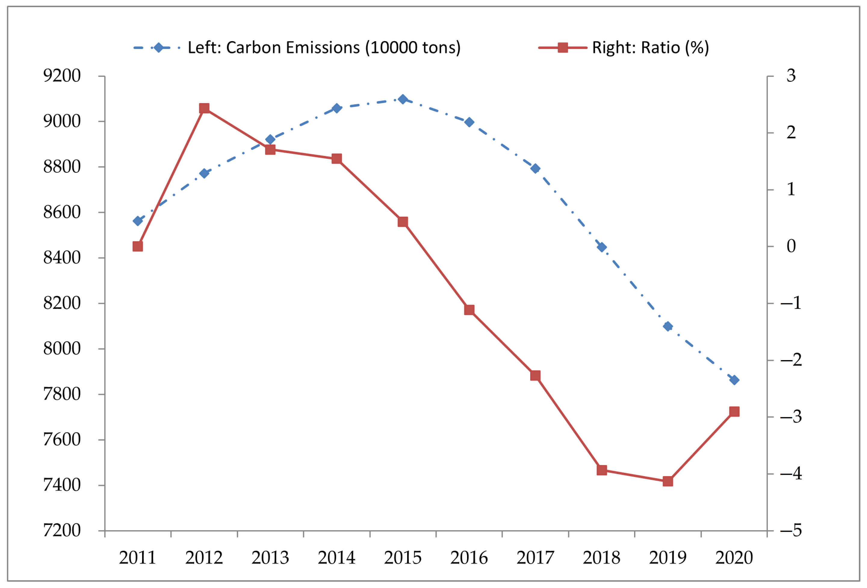
Figure 2.
Spatial distribution of China’s AGTFP in 2012, 2016, and 2020.


Table 1.
Main sources and coefficient of carbon emission in agricultural production.
| Sources | Coefficient | Reference |
|---|---|---|
| Chemical fertilizer | 0.8956 kg kg−1 | Oak Ridge National Laboratory, ORNL |
| Pesticides | 4.9341 kg kg−1 | ORNL |
| Agricultural film | 5.18 kg kg−1 | Institute of Resources, Ecosystem and Environment of Agriculture, IREEA |
| Diesel | 0.5927 kg kg−1 | Intergovernmental Panel on Climate Change, IPCC |
| Plowing | 312.6 kg km−2 | Institute of Agriculture and Biotechnology of China Agricultural University, IABCAU |
| Irrigation | 25 kg ha−1 | Dubey and Lal [57] |
Note: According to the data in China Statistical Yearbook from 2011–2019, the average proportion of thermal power generation is 0.7413; thus, the actual coefficient of irrigation is 18.5333 kg ha−1.
Table 2.
Descriptive statistics.
| Variables | Definition | Mean | S.D |
|---|---|---|---|
| Output variables | |||
| Agricultural output (Expected output) | The gross agricultural output value (based on 2011) (100 million CNY) | 1493.201 | 1053.501 |
| Carbon emissions (Unexpected output) | Carbon emissions in agricultural activities (10,000 tons) | 279.411 | 198.865 |
| Input variables | |||
| Land | Total planting area of crops (1000 ha) | 5336.927 | 3816.424 |
| Labor | Agricultural employees (10,000 individuals) | 782.335 | 553.471 |
| Machinery | The total power of agricultural machinery (10,000 kW) | 3318.604 | 2924.103 |
| Water | Irrigation area (1000 ha) | 2127.971 | 1667.872 |
| Energy | Diesel consumption in agriculture (10,000 tons) | 66.752 | 57.919 |
| Chemical fertilizer | The use of chemical fertilizer (10,000 tons) | 185.888 | 147.006 |
| Pesticides | The use of pesticides (10,000 tons) | 7.983 | 6.725 |
| Agricultural films | The use of agricultural plastic films (10,000 tons) | 5.351 | 4.185 |
| Empirical variables | |||
| lnC | The logarithm of agricultural carbon emissions | 5.202 | 1.154 |
| GML | AGTFP | 1.016 | 0.047 |
| GTC | Agricultural green technology change | 1.020 | 0.041 |
| GEC | Agricultural green efficiency change | 0.997 | 0.035 |
| pol | The policy of ‘Action Plan for the zero increase of fertilizer use and pesticides by 2020’, 0 = No, 1 = Yes | 0.600 | 0.491 |
| ser | The output value of agricultural services (100 million CNY, based on 2011)/planting area of crops (1000 ha) | 0.014 | 0.009 |
| pgdp | GDP per capita (100 million CNY, based on 2011) | 4.112 | 1.831 |
| agri | Added value of primary industry (100 million CNY)/GDP (100 million CNY) | 0.097 | 0.051 |
| mac | The total power of agricultural machinery (10,000 kW)/planting area of crops (1000 ha) | 0.685 | 0.350 |
| labor | Agricultural employees (10,000 individuals) /planting area of crops (1000 ha) | 0.168 | 0.069 |
Table 3.
The effect of government policy on carbon emissions.
| Variables | Coef. | S.D |
|---|---|---|
| Government policy (Action Plan for the zero increase of fertilizer use and pesticides by 2020) | −0.062 *** | 0.013 |
| pgdp | −0.013 | 0.016 |
| agri | 0.417 | 0.531 |
| mac | 0.144 ** | 0.064 |
| labor | −0.580 *** | 0.199 |
| Constant | 5.253 *** | 0.099 |
| F | 7.24 *** | |
| Obs | 310 |
Note: ** and *** indicate significance levels at 5% and 1%, respectively.
Table 4.
The AGTFP index of China and 31 provinces (2011–2020).
| Region | 2011 | 2012 | 2013 | 2014 | 2015 | 2016 | 2017 | 2018 | 2019 | 2020 |
|---|---|---|---|---|---|---|---|---|---|---|
| China | 1.000 | 1.040 | 1.027 | 1.000 | 0.999 | 1.001 | 0.947 | 1.014 | 1.017 | 1.024 |
| Beijing | 1.000 | 1.036 | 1.050 | 1.036 | 1.013 | 1.021 | 1.052 | 1.134 | 1.005 | 1.000 |
| Tianjin | 1.000 | 1.029 | 1.034 | 1.021 | 1.012 | 0.989 | 0.915 | 1.127 | 1.026 | 1.233 |
| Hebei | 1.000 | 1.037 | 1.067 | 0.965 | 0.974 | 1.007 | 0.891 | 1.047 | 1.022 | 1.077 |
| Shanxi | 1.000 | 1.009 | 1.022 | 1.010 | 0.992 | 0.992 | 0.981 | 1.009 | 1.005 | 1.032 |
| Inner Mongolia | 1.000 | 1.005 | 1.001 | 0.998 | 0.977 | 0.992 | 0.999 | 1.019 | 1.022 | 1.063 |
| Liaoning | 1.000 | 1.037 | 1.007 | 1.010 | 1.031 | 1.000 | 0.926 | 1.034 | 1.029 | 1.031 |
| Jilin | 1.000 | 1.018 | 1.003 | 0.994 | 0.995 | 0.941 | 0.901 | 1.022 | 0.998 | 1.057 |
| Heilongjiang | 1.000 | 1.079 | 1.076 | 0.983 | 0.958 | 0.973 | 1.088 | 1.016 | 1.051 | 1.040 |
| Shanghai | 1.000 | 1.004 | 1.043 | 0.970 | 1.007 | 1.007 | 0.996 | 1.175 | 1.000 | 1.000 |
| Jiangsu | 1.000 | 1.064 | 1.025 | 1.005 | 1.061 | 0.993 | 0.983 | 0.994 | 1.003 | 1.033 |
| Zhejiang | 1.000 | 1.041 | 1.056 | 1.011 | 1.009 | 1.038 | 0.994 | 1.002 | 1.036 | 1.000 |
| Anhui | 1.000 | 1.003 | 1.007 | 1.001 | 0.990 | 1.009 | 0.990 | 1.000 | 1.013 | 1.065 |
| Fujian | 1.000 | 1.047 | 1.013 | 1.039 | 1.009 | 1.079 | 0.964 | 1.018 | 1.019 | 1.000 |
| Jiangxi | 1.000 | 1.022 | 1.051 | 1.005 | 1.028 | 1.038 | 0.985 | 1.030 | 1.036 | 1.033 |
| Shandong | 1.000 | 1.005 | 1.083 | 1.006 | 0.989 | 0.900 | 0.957 | 1.028 | 1.031 | 1.037 |
| Henan | 1.000 | 1.040 | 1.008 | 1.024 | 0.972 | 0.942 | 0.987 | 1.061 | 1.044 | 1.100 |
| Hubei | 1.000 | 1.033 | 1.002 | 0.980 | 0.965 | 1.016 | 0.982 | 1.009 | 1.071 | 1.072 |
| Hunan | 1.000 | 1.036 | 0.981 | 1.003 | 0.998 | 1.019 | 0.835 | 0.996 | 1.088 | 1.105 |
| Guangdong | 1.000 | 1.031 | 1.051 | 1.003 | 1.013 | 1.058 | 0.961 | 0.980 | 1.062 | 1.000 |
| Guangxi | 1.000 | 0.987 | 1.001 | 0.993 | 1.006 | 1.019 | 1.045 | 1.035 | 1.057 | 0.987 |
| Hainan | 1.000 | 1.042 | 0.961 | 1.080 | 1.000 | 1.000 | 0.971 | 1.006 | 1.023 | 1.000 |
| Chongqing | 1.000 | 1.033 | 1.014 | 0.998 | 1.004 | 1.062 | 0.963 | 1.052 | 1.022 | 1.055 |
| Sichuan | 1.000 | 1.008 | 0.977 | 0.994 | 1.030 | 0.996 | 1.005 | 0.990 | 0.997 | 1.013 |
| Guizhou | 1.000 | 1.040 | 1.031 | 1.136 | 1.153 | 1.004 | 1.000 | 0.990 | 1.010 | 1.000 |
| Yunnan | 1.000 | 1.040 | 1.029 | 1.006 | 0.972 | 0.990 | 0.981 | 1.179 | 1.089 | 0.958 |
| Tibet | 1.000 | 1.000 | 1.000 | 0.889 | 0.934 | 1.204 | 0.933 | 1.072 | 1.000 | 1.000 |
| Shaanxi | 1.000 | 1.019 | 1.059 | 1.022 | 0.951 | 1.020 | 0.956 | 1.027 | 1.023 | 1.062 |
| Gansu | 1.000 | 1.019 | 1.015 | 0.994 | 1.000 | 1.028 | 0.916 | 1.027 | 1.027 | 1.016 |
| Qinghai | 1.000 | 0.994 | 0.998 | 0.992 | 0.991 | 1.022 | 0.998 | 1.020 | 1.182 | 1.142 |
| Ningxia | 1.000 | 0.997 | 1.051 | 1.036 | 1.081 | 1.003 | 0.985 | 1.174 | 0.950 | 1.197 |
| Xinjiang | 1.000 | 1.016 | 0.930 | 0.937 | 0.955 | 0.993 | 1.022 | 1.051 | 1.040 | 1.099 |
Table 5.
Regression results of AGTFP and its decomposition.
| Variables | GML | GTC | GEC | |||
|---|---|---|---|---|---|---|
| FE | IV-2SLS | FE | IV-2SLS | FE | IV-2SLS | |
| ser | 1.498 ** (0.590) | 2.823 *** (0.863) | 0.969 * (0.513) | 1.948 *** (0.748) | 0.550 (0.441) | 0.872 (0.639) |
| pgdp | −0.014 * (0.008) | −0.018 ** (0.008) | −0.016 ** (0.007) | −0.019 *** (0.007) | 0.001 (0.006) | −0.0004 (0.006) |
| agri | 0.372 (0.249) | 0.503 * (0.258) | 0.087 (0.216) | 0.183 (0.224) | 0.260 (0.186) | 0.292 (0.191) |
| mac | 0.016 (0.031) | 0.004 (0.033) | 0.021 (0.028) | 0.012 (0.028) | −0.005 (0.024) | −0.008 (0.024) |
| labor | −0.281 *** (0.095) | −0.307 *** (0.096) | −0.108 (0.082) | −0.127 (0.084) | −0.165** (0.071) | −0.171 ** (0.071) |
| Constant | 1.052 *** (0.045) | 1.051 *** (0.045) | 1.066 *** (0.039) | 1.065 *** (0.039) | 0.992 *** (0.034) | 0.992 *** (0.034) |
| Within R-squared | 0.055 | 0.038 | 0.031 | 0.018 | 0.025 | 0.023 |
| Obs | 310 | 310 | 310 | 310 | 310 | 310 |
Note: *, **, and *** indicate significance levels at 10%, 5%, and 1%, respectively.
Table 6.
Heterogeneity analysis based on Heihe–Tengchong line.
| Variables | East Region of Heihe–Tengchong Line | West Region of Heihe–Tengchong Line | ||||
|---|---|---|---|---|---|---|
| GML | GTC | GEC | GML | GTC | GEC | |
| ser | 1.487 ** (0.577) | 1.060 ** (0.466) | 0.460 (0.471) | 2.015 (3.457) | 2.674 (3.554) | −0.621 (2.128) |
| pgdp | −0.012 (0.008) | −0.017 ** (0.007) | 0.003 (0.007) | 0.002 (0.022) | 0.005 (0.022) | −0.003 (0.013) |
| agri | 0.324 (0.258) | 0.157 (0.208) | 0.152 (0.211) | 1.320 * (0.704) | 0.417 (0.724) | 0.829 * (0.434) |
| mac | −0.019 (0.035) | −0.005 (0.028) | −0.013 (0.029) | 0.035 (0.071) | 0.047 (0.073) | −0.010 (0.044) |
| labor | −0.120 (0.097) | −0.008 (0.079) | −0.109 (0.080) | −1.270 *** (0.298) | −0.673 ** (0.306) | −0.556 *** (0.183) |
| Constant | 1.050 *** (0.046) | 1.068 *** (0.037) | 0.989 *** (0.038) | 1.028 *** (0.142) | 1.008 (0.146) | 1.022 *** (0.088) |
| F | 1.91 * | 2.18 * | 0.67 | 4.21 *** | 1.44 | 2.55 ** |
| Obs | 230 | 230 | 230 | 80 | 80 | 80 |
Note: *, **, and *** indicate significance levels at 10%, 5%, and 1%, respectively.
Publisher’s Note: MDPI stays neutral with regard to jurisdictional claims in published maps and institutional affiliations. |
© 2022 by the authors. Licensee MDPI, Basel, Switzerland. This article is an open access article distributed under the terms and conditions of the Creative Commons Attribution (CC BY) license (https://creativecommons.org/licenses/by/4.0/).
Share and Cite
MDPI and ACS Style
Xu, Q.; Zhu, P.; Tang, L. Agricultural Services: Another Way of Farmland Utilization and Its Effect on Agricultural Green Total Factor Productivity in China. Land 2022, 11, 1170. https://doi.org/10.3390/land11081170
AMA Style
Xu Q, Zhu P, Tang L. Agricultural Services: Another Way of Farmland Utilization and Its Effect on Agricultural Green Total Factor Productivity in China. Land. 2022; 11(8):1170. https://doi.org/10.3390/land11081170
Chicago/Turabian StyleXu, Qinhang, Peixin Zhu, and Liang Tang. 2022. "Agricultural Services: Another Way of Farmland Utilization and Its Effect on Agricultural Green Total Factor Productivity in China" Land 11, no. 8: 1170. https://doi.org/10.3390/land11081170
Note that from the first issue of 2016, this journal uses article numbers instead of page numbers. See further details here.