

Land Subsidence Detection in the Coastal Plain of Tabasco, Mexico Using Differential SAR Interferometry

1
Instituto Politécnico Nacional, Centro Interdisciplinario de Ciencias Marinas, Av. Instituto Politécnico Nacional S/N, Col. Playa Palo de Santa Rita, La Paz 23096, BCS, Mexico
2
CICESE, Carretera Ensenada-Tijuana No. 3918, Zona Playitas, Ensenada 22860, BC, Mexico
*
Author to whom correspondence should be addressed.
Land 2022, 11(9), 1473; https://doi.org/10.3390/land11091473
Submission received: 3 July 2022
/
Revised: 28 August 2022
/
Accepted: 29 August 2022
/
Published: 3 September 2022
(This article belongs to the Special Issue Land Surface Monitoring Based on Satellite Imagery)
Abstract
:Land subsidence (LS) increases flood vulnerability in coastal areas, coastal plains, and river deltas. The coastal plain of Tabasco (TCP) has been the scene of recurring floods, which caused economic and social damage. Hydrocarbon extraction is the main economic activity in the TCP and could be one of the causes of LS in this region. This study aimed to investigate the potential of differential SAR interferometric techniques for LS detection in the TCP. For this purpose, Sentinel-1 SLC descending and ascending images from the 2018–2019 period were used. Conventional DInSAR, together with the differential interferograms stacking (DIS) approach, was applied. The causes of interferometric coherence degradation were analyzed. In addition, Sentinel-1 GRD images were used for delimitation of areas recurrently affected by floods. Based on the results of the interferometric processing, several subsiding zones were detected. The results indicate subsidence rates of up to −6 cm/yr in the urban centers of Villahermosa, Paraíso, Comalcalco, and other localities. The results indicate the possibility of an influence of LS on the flood vulnerability of the area south of Villahermosa city. They also suggest a possible relationship between hydrocarbon extraction and surface deformation.
1. Introduction
Land subsidence (LS) is a major worldwide hazard, and it is defined as the down-ward, mainly vertical, displacement of the Earth’s surface relative to a stable reference level [1,2]. LS is caused by a wide variety of processes of natural and anthropogenic origin. The natural-driven processes, such as glacial isostatic adjustment (GIA) [3,4], tectonic movements (except co-seismic displacement) [5,6], and sediment compaction [7,8], often cause a slow and steady motion (a few mm/yr). Human activities that cause subsidence include withdrawal of groundwater [9,10,11,12], hydrocarbons [13,14,15], geothermal water, and brine [16,17,18]; mining [19,20,21]; loading of engineered structures [22,23]; and wetland drainage [24]. Generally, the observed rates of human-induced subsidence greatly exceed the rates of natural subsidence, reaching centimeters per year, to even meters per year (e.g., mining activities [25]). LS damage to urban and civil infrastructure causes constant and considerable economic losses. However, the most notable impact of LS is produced in coastal areas, coastal plains, and river deltas, where LS increases flood vulnerability (flood frequency, inundation depth, and duration of floods) [26,27,28]. Identifying LS-prone areas and estimating their rate and spatial extension is essential in this phenomenon’s assessment and management.
The use of satellite data and remote sensing (RS) techniques is a common practice in Earth surface observations. The advantages of satellite RS techniques are their comprehensive area coverage, non-invasiveness, and cost-effectiveness. In particular, the differential interferometric synthetic aperture radar (DInSAR) technique has become an effective RS tool for monitoring and assessing the Earth surface displacements induced by a variety of geophysical and geological processes, including earthquakes, volcanoes, landslides, LS, and sinkholes, among others [29]. The DInSAR technique is based on acquiring complex SAR images over the same area at different times using repeated passes. The standard DInSAR approach (or conventional DInSAR) exploits the phase difference of the SAR image pairs, providing a measurement of surface displacements occurring between the two acquisitions with a sub-centimetric accuracy and a decametric spatial resolution (e.g., [30,31,32]).
The uncertainties in the measurement of conventional DInSAR, due to the contribution of non-displacement signals, such as the digital elevation model (DEM) and orbitals errors, and atmospheric delay, are the handicaps of this approach [33]. In addition, the temporal and geometrical decorrelation limit its practical applications [34]. Advanced-DInSAR techniques, based on large stacks composed of many SAR images, partly overcome DInSAR limitations (e.g., [35,36,37]). Despite the considerable advances in DInSAR processing techniques, applying DInSAR for displacement measurements in areas where the conditions of the land surface change significantly, e.g., densely vegetated areas, remains challenging.
Tabasco is an oil-rich state located in the southeast of Mexico; its northern border runs along the Gulf of Mexico. Much of the state is a wide alluvial coastal plain, the so-called Tabasco Coastal Plain (TCP). Due to its climatic and hydro-geologic conditions, Tabasco is one of the most flood-prone Mexican states [38,39]. The state’s high incidence of floods has been exacerbated by sea-level rises and possibly LS, through natural or anthropogenic effects. LS is not considered a high-risk phenomenon in the Tabasco state. The LS phenomenon has been poorly investigated, and its effects on the increase of TCP area’s vulnerability to flooding and coastal erosion is unknown. Hydrocarbon production is the main economic activity in the region, with more than a thousand wells distributed in 106 oil fields, so the possibility of significant anthropogenic subsidence occurrence cannot be discarded and must be investigated in detail.
DInSAR techniques have proven practical LS detection and monitoring tools in coastal areas (e.g., [26,40,41,42,43,44,45]). However, to the authors’ knowledge, there are not formal papers published or submitted to journals where DInSAR was applied to investigate LS in Tabasco. Early DInSAR results for the Tabasco region were published only as a conference paper [46]. Therefore, this study evaluates DInSAR’s potential for land subsidence detection and monitoring in the TCP. Conventional DInSAR and the interferograms stacking procedure (A-DInSAR) were applied to identify the Earth’s surface displacement in TCP. Sentinel-1 data from January 2018 to January 2020 were used. The achieved results allowed the identification of land sinking areas during the period covered by the study, which should be the target of more detailed investigations.
2. Materials and Methods
2.1. Study Area
This study’s area of interest (AOI) belongs to the TCP, a tropical lowland on the Gulf of Mexico, in Tabasco State, southeastern Mexico (Figure 1). It is part of the Mexican physiographic province called the Southern Coastal Plain of the Gulf of Mexico [47]. It was formed by alluvial sediments brought by rivers from the mountains of Chiapas (Mexico) and Guatemala; the rivers cross the state to flow into the Gulf of Mexico. The land is largely covered with lakes, lagoons, and wetlands (floodable areas), one of the most important in Mexico. About 80% of the TCP surface is composed of marsh, alluvial, coastal, and lake deposits from the Quaternary period; corresponding with the development of the current environments, from the Pliocene to today, and about 20% is made up of sedimentary rock from the Tertiary period [48,49,50]. The soils of the TCP are predominantly of alluvial and organic origin, such as Gleysols, Histosols, and Fluvisols [50,51], and are characterized by a poor drainage capacity.
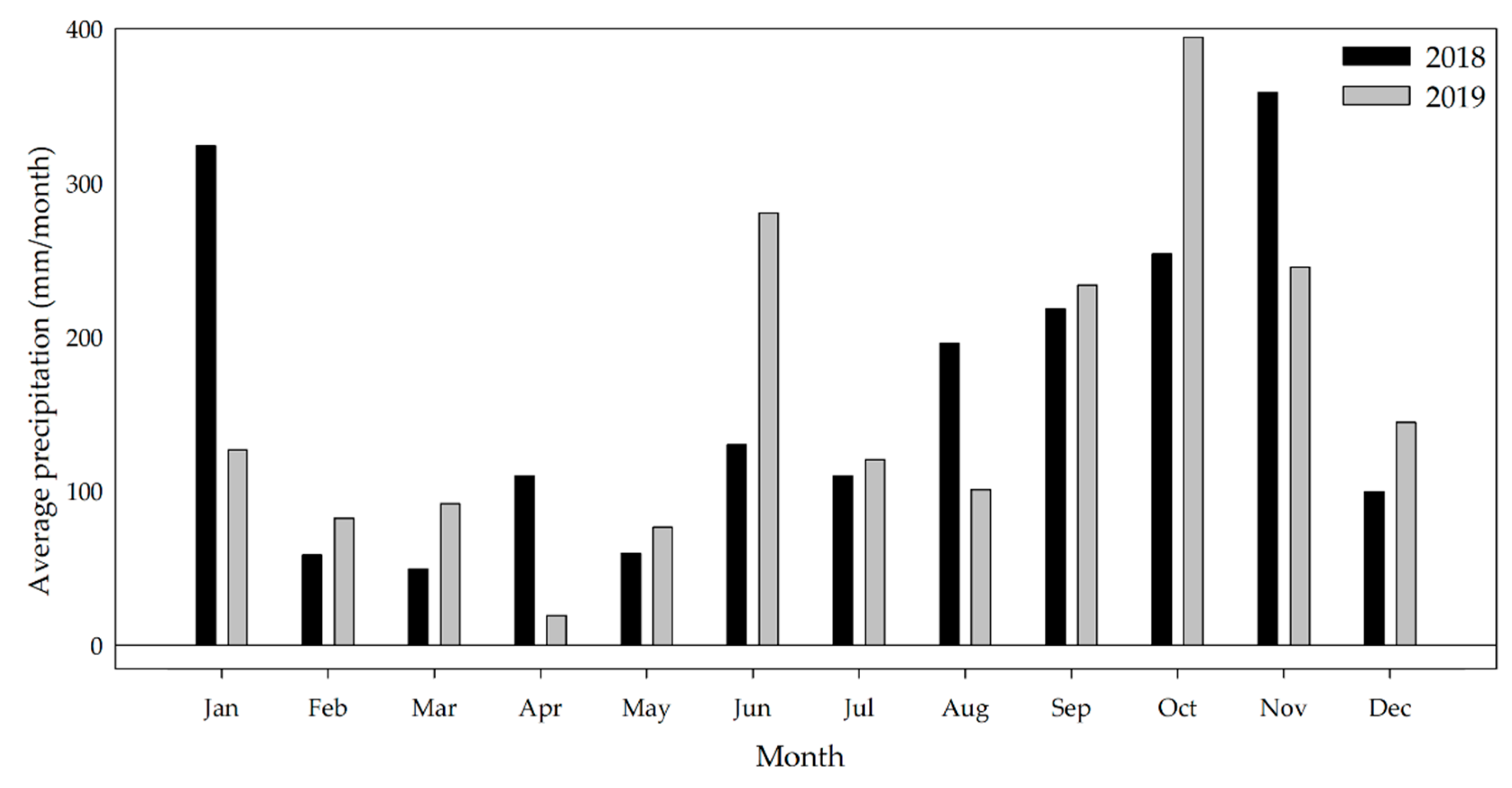
The TCP region has a tropical rainforest climate, designated as Af under the Köppen-Geiger climate classification system. This region’s average annual air temperature is 26 °C, with average monthly temperatures ranging between 22.7 °C (January) and 28.9 °C (May). The TCP receives 1500–2000 mm of annual precipitation, mainly in the rainy season between June and November [52]. Furthermore, the region is regularly subjected to tropical storms and hurricanes from the Gulf of Mexico and the Pacific Ocean. The monthly average precipitation in the analyzed period (2018–2019) is presented in Figure 2.
Due to TCP’s climatic and hydro-geologic conditions, its territory is exposed to floods annually [39]. Some floods have been catastrophic, such as those of 1980, 1995, 2007 [53], and 2020 [54]. The extensive flooding that occurred in 2020, at the end of October and early November, affected over 62% of the Tabasco state and more than 1.2 million people [54].
Figure 2.
Monthly average precipitation (data available at [55]).
Figure 2.
Monthly average precipitation (data available at [55]).
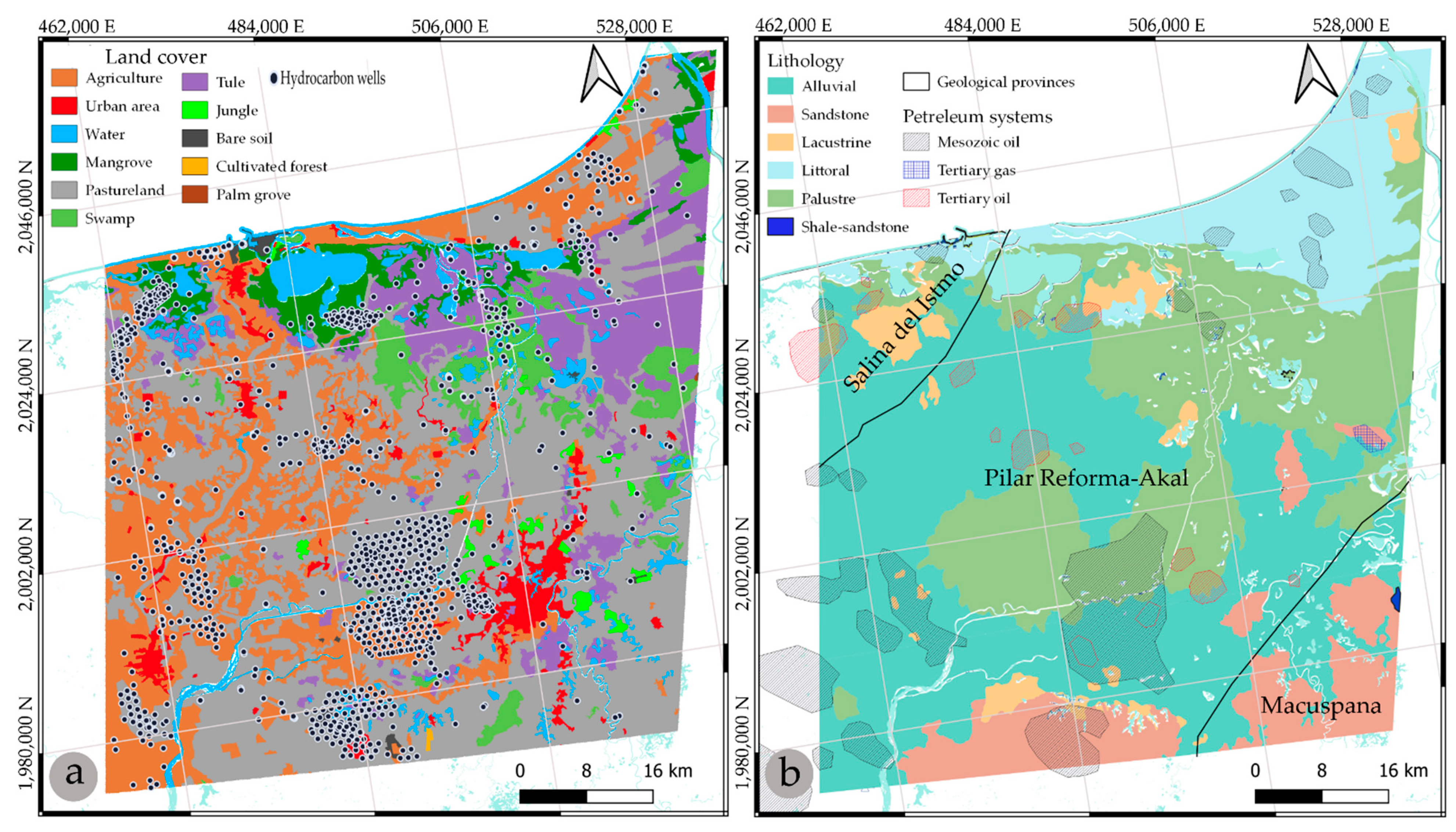
The AOI covers 596,573 ha, of which 69.76% are dedicated to economic activities, and 22.01% are covered by natural vegetation. The natural vegetation in TCP is represented by tropical rainforest and various wetland communities, including mangroves. The most important economic activities for the state of Tabasco are oil and gas production, agriculture, and livestock. Tabasco is a mainly rural state; agricultural fields and pastures cover approximately 69% of the area used for economic activities, and only 3.48% is urban (Figure 3a).
Since large-scale exploitation of hydrocarbon resources began at the end of the 1950s, oil and gas production has become Tabasco’s economic mainstay. At present, Tabasco is a leader in hydrocarbon reserves and is one of Mexico’s primary oil-producer states. Figure 3a shows the hydrocarbon extraction wells distribution over the AOI. Most wells have a depth ranging from 1500 to 3500 m. However, some wells reach up to 7615 m.
The study area is part of the Salina de Istmo, Pilar Reforma-Akal, and Macuspana basins (Figure 3b). The Salina de Istmo basin is Miocene-Pliocene and associated with a system of normal faults, including the Comalcalco sub-basin, associated with sediment loading and salt evacuation. The Macuspana basin is from the early Miocene-Pliocene. Sedimentary facies vary from fluviodeltaic to marine and are characterized by turbidite deposition. The Pilar Reforma-Akal Basin is the most representative of the study area where hydrocarbons are stored in limestone from the Upper Cretaceous and Upper Jurassic [56,57]. The hydrocarbon system’s distribution corresponds to the Mesozoic oil fields and, to a lesser extent, to the Tertiary (Figure 3b) [57].
High volume extraction of hydrocarbons can cause LS around the producing wells. Land surface sinking due to oil and gas production depends on the geometrical shape and thickness of the reservoir, the compaction coefficient, the pressure drops in the reservoir, and the geomechanical behavior of the overburden [58]. The documented rates of LS caused by hydrocarbon extraction range from a few mm/yr [59] to up to 0.75 m/yr [60]. Even a small subsidence in plain areas could significantly increase flood vulnerability.
Figure 3.
Physical-geographical characteristics of AOI; (a) land cover (INEGI [61] and distribution of hydrocarbon wells (IICNIH [62]). The area with the highest well density is located west of Villahermosa, with wells depth ranging between 1500 and 3500 m; (b) Lithology, geological provinces, distribution of the oil system, and its geological era [57,62].
2.2. Data
In this study, Sentinel-1 level-1 images provided in the Single Look Complex (SLC) format [63] by the Alaska Satellite Facility (https://asf.alaska.edu, accessed on 2 December 2019) were used in DInSAR processing. The Copernicus Sentinel-1 mission, developed by the European Space Agency (ESA), is based on a constellation of two satellites: Sentinel-1A, launched in April 2014, and Sentinel-1B, launched in April 2016. The Sentinel-1 constellation operates at the C-Band frequency (5.405 GHz, 5.5 cm wavelength), with a 12-day repeated acquisition for a single mission, and 6-days in the case of a two-satellite combination. Sentinel-1 imagery was selected in this study, thanks to its free accessibility with a regularly repeated acquisition at a 6-day interval.
A total of 115 (Sentinel-1A/1B) images were acquired on ascending Path 34, Frame 54/55, in Interferometric Wide (IW) swath mode, with dual (VV + VH) polarization between 2 January 2018 and 29 December 2019. Moreover, 108 images were acquired on descending Path 99, Frame 530/532, in IW swath mode [64,65,66], with dual polarization between 6 January 2018 and 27 December 2019. Only Sentinel-1 VV polarization bands were used, since co-polarized bands provide higher coherence than VH polarization. The main characteristics of the Sentinel-1 SLC data used in this study for DInSAR processing are listed in Table 1.
The external datasets used for the SAR SLC data interferometric processing include the Shuttle Radar Topographic Mission (SRTM) 1-arc-second (30 m) DEM [67] and Copernicus Sentinel-1A and Sentinel-1B precise orbital files (AUX_POEORB products), obtained from the Copernicus Open Access Hub.
Satellite data available for mapping and monitoring flood coverage were obtained by passive (e.g., onboard Landsat, Aqua, Sentinel-2, Resourcesat-2) and active (e.g., Sentinel-1, RADARSAT, ENVISAT) sensors [68,69]. Sentinel-1 level-1 ground range detected (GRD) images were obtained from the Alaska Satellite Facility and used to identify flooded areas. Sentinel-1 level-1 (GRD) products consist of focused SAR data that has been detected, analyzed, and projected to the ground range using a ground ellipsoid model. The pixel values of the Sentinel-1 level-1 (GRD) image represent the detected amplitude of the backscattered signal, without phase information. Two pairs of GRD images with dual-polarization from descending orbital pass were acquired, covering the flood events in 2018 and 2019. Only VV polarization bands were used because, for flooded area detection, the co-polarization comparison gives better results than the cross-polarization one, while the use of VV polarization is recommended over the use of VH data [70]. The characteristics of the Sentinel-1 GRD products used in this study are presented in Table 2.
2.3. SAR Differential Interferometry Background
The fundamentals of the conventional DInSAR technique have been presented in many publications [29,31,70]. Therefore, only some aspects relevant to this study are briefly described.
In principle, SAR interferometry exploits the information in the interferometric phase, calculated as the phase difference between two coregistered SAR images acquired from slightly different orbit positions (spatial baseline) and different times (temporal baseline). The interferometric phase () is the sum of contributions from several factors, and the following equation can express this:
where represents the phase due to surface displacement, refers to the phase caused by local topography (or topographic phase), is the phase produced by a surface of constant elevation on a spherical Earth (curved Earth), also known as the orbital phase, denotes the phase components due to the variation of atmospheric conditions between the image acquisitions (the so-called atmospheric phase screen (APS)), and includes all the phase noise contributions that corrupt the interferometric SAR signal.
All other contributors to the interferometric phase must be removed or diminished, to obtain the Earth surface displacement measurement. Using external DEM and precise orbital information, phase contributions caused by topography and the curved Earth can be estimated and removed from the interferometric phase. This is the basic concept of the Differential SAR Interferometry (DInSAR) approach. However, the differential interferometric phase can still contain some “unwanted” phase components. APS is one of the main sources of errors that influence the differential interferometric phase, and it can degrade the accuracy of surface displacement estimates using DInSAR. Topographic and orbital errors can also contribute to the differential interferometric phase.
The accuracy of surface displacement measurements from DInSAR greatly depends on the quality of the differential interferometric phase. The established criterion to measure the quality of the differential interferometric phase is the value of the complex correlation coefficient, the so-called coherence. The coherence is a measure of phase correlation (or phase reliability) between two complex SAR images, M (master image) and S (slave image), and is defined as [71]:
where is the complex conjugate of the complex slave image , and are the amplitude of complex SAR master and slave image, respectively, and indicates the spatial set of samples employed in the coherence estimation. The coherence values lie in the range ; a value of zero indicates complete incoherence and a differential interferometric phase value with no useful information, whereas a value of one indicates complete coherence and a differential interferometric phase value with no noise. DInSAR is effectively applied only in areas where the differential interferometric phase is characterized by high coherence. The main factors that affect the coherence are temporal and spatial decorrelation and low accuracy of image coregistration.
The temporal decorrelation phenomenon is caused by changes in the physical and geometric properties of the scatterers on the Earth’s surface [72]. Some of the main sources of temporal decorrelation are erosion, vegetation growth, cultivation, snow, and near-surface moisture changes.
Spatial or geometric decorrelation may result from high variations in imaging geometry. Thus, images with a short spatial baseline must be selected for interferometric processing.
A practical way to overcome the conventional DInSAR limitations mentioned above is combining the information from multiple short-interval differential interferograms, to extract common information. The most basic procedure is to compute integer linear combinations of unwrapped differential interferograms [33] or perform their temporal averaging, the so-called differential interferograms stacking (DIS) approach. The main assumption of this method is that the deformation phase is highly correlated, and the error/noise terms (e.g., APS, signal noise, orbital errors, and nonlinear ground displacements) are uncorrelated between independent pairs. The application of this method increases the signal-to-noise ratio (SNR) and improves the reliability of the Earth surface displacement measurements [73].
2.4. DInSAR Processing
The GAMMA software package developed by GAMMA Remote Sensing and Consulting AG, Bern, Switzerland [74] was used for S1 Level-1 SLC product processing. The processing chain was divided into three stages: pre-processing, conventional repeat-pass DInSAR, and stacking. Pre-processing and conventional repeat-pass DInSAR were performed following the standard workflow used for processing S1 TOPS mode image pairs. This workflow is comprehensively explained in [75].
The pre-processing stage consisted of importing SLC data; updating of image metadata with precise orbital state vectors; S1 TOPS splitting, which included polarization selection; selection of sub-swaths and bursts covering the AOI; and selection of suitable S1 SLC image pairs and coregistration. Here, suitable S1 SLC image pairs were selected within the thresholds of the perpendicular and temporal baselines, which were set to 200 m and 18 days, respectively. The connection graph for ascending and descending datasets generated using these thresholds is presented in Figure 4a,b, respectively. A total of 321 ascending and 290 descending interferograms were generated and used in the stacking procedure. However, for coherence analysis, one additional interferogram from a descending orbital pass with a temporal baseline of 24 days was generated.
The conventional repeat-pass DInSAR stage included the formation of interferograms, multi-looking, simulation of topographic phases, differential interferogram generation, coherence calculation, phase filtering, phase unwrapping, orbital error correction, atmospheric correction, phase to displacement conversion, and interferometric product (i.e., coherence, differential interferograms, displacements map) geocoding (Latitude/Longitude WGS84 coordinate system).
Topographic phases were simulated using the precise orbits and an external DEM. Differential interferograms were formed at a default 2 looks in azimuth and 10 looks in range, to obtain a pixel size of ~40 × 40 m2. To improve the quality of differential interferograms and optimize the phase unwrapping procedure, the differential interferograms were filtered using an adaptive Goldstein filter [76], with an optimal filter strength of 0.7 being employed in this study, after a number of trials. After phase filtering, a minimum-cost flow (MCF) algorithm [77,78] was used for phase unwrapping. Areas with a coherence smaller than 0.2 were masked out before unwrapping. The linear trend was estimated and subtracted from the unwrapped differential interferograms, to correct the residual linear ramp caused by orbital errors. Differential atmospheric delay in the interferometric phase, which is correlated with the topography, was reduced using the empirical phase-based method, for which the linear correlation between the unwrapped phase and the elevation of DEM was calculated [79,80].
During the stacking stage, the unwrapped differential interferograms of each set were summed and divided by the total (cumulative) time interval of all interferograms of the set in years, to obtain an average annual LOS displacement rate. Before stacking, the interferograms were referenced to a common (32 × 32 pixels) area and were shifted accordingly, to set the reference phase to zero. The common reference area was in the center of Villahermosa.
After stacking, phase to displacement conversion was performed, and the resulting LOS displacement rate maps were geocoded.
2.5. Identification of Flooded Areas
Sentinel-1 GRD images were pre-processed by implementing radiometric calibration, spot filtering, and geometric correction of the data, to identify flooded areas. Radiometric calibration was initially applied, as it is an essential step in SAR GRD image pre-processing. The pixel values of the images could directly represent the radar backscatter [81], achieving results in dB. Image pixels representing bodies of water have a lower radar backscatter coefficient than other features [82], such as land or vegetation. The effects of thermal noises were also removed, and a precise orbit file was applied to the images. Lee Sigma filtering was applied to reduce the speckle noise caused by random effects of multiple backscattering within each resolution cell, which is best suited for this processing [81], leading to better results, with a filter size of 7 × 7. Finally, atmospheric correction was performed, to compensate for topography variations caused by the satellite sensor’s viewing angle [81,82].
To obtain the flooded areas, the thresholding method was used, which is the simplest method of image segmentation [83]. Here, the areas affected by flooding were identified for two flood events: February 2018 and November 2019. The binary images (water/non-water) were created using thresholds estimated from intensity (in dB) histograms of pre-processed Sentinel-1 GRD images. The used threshold values varied for the analyzed images between −12 and −10 dB; the water areas being those with an intensity below the applied threshold’s value. To separate the permanent water bodies from the areas affected by floods, the permanent water bodies were identified using pre-flood event images (dry conditions) and then masked out in co-flood event binary images, so that, as a result, binary images of areas affected/non-affected by floods were obtained.
A permanent water bodies mask was also used to exclude water bodies from interferometric coherence analysis, as water bodies generally have a low coherence (near zero).
SNAP software (Sentinel Application Platform) [84] was used for pre-processing, whereas GIS software was used to obtain the flooded areas from the pre-processed images.
3. Results
3.1. Coherence Analysis
As mentioned above, DInSAR can only be effectively applied in areas where the differential interferometric phase is characterized by high coherence. For a short spatial baseline interferometric pair, where two images are coregistered with high accuracy, the temporal decorrelation is the main factor of the coherence degradation.
To investigate the impact of the temporal baseline on the quality of interferometric results in the AOI, differential interferograms with a temporal baseline of 6, 12, 18, and 24 days and the common master image (12 February 2019) were processed, and their coherences were estimated (Figure 5 and Figure 6). All image pairs had a short perpendicular baseline, to avoid the influence of spatial decorrelation on coherence degradation. All four analyzed image pairs covered relatively dry periods, without important or extreme precipitation (Figure 2) or floods. The parameters of interferometric pairs are presented in Table 3.
As it can be seen in Figure 5, the AOI is characterized by low coherence values, even for minimal possible temporal separation between images (6 days). The vegetation dominated areas, as for AOI, are especially likely to lose their coherence within a very short period. Moreover, an important loss of coherence is observed with a temporal baseline increase.
Figure 6 shows the coherence histograms for selected interferometric pairs (Figure 5; Table 3). As the temporal baseline increases, the frequency of pixels with low coherence also increases, whereas the mean coherence decreases from 0.13 (6 days) to 0.08 (24 days).
Figure 7 shows the average images for the ascending and descending orbital pass and associated coherence histograms. For each orbital direction, the average coherence image was obtained by averaging the coherence of all image pairs processed. These interferometric pairs correspond to the 2018–2019 period and meet the established baseline thresholds. The histograms (Figure 7c) show that the study area is dominated by low coherence (≤0.2), due to the land cover type (different types of vegetation). The highest values of average coherence (>0.3) correspond to urban areas and bare soil, reaching up to 0.99.
The average coherence values for different land cover classes are presented in Figure 8. In this case, the average coherence per class (ACC) value was calculated for each processed image pair.
As can be seen in Figure 8, the point cloud of ACC values is separated into two groups. The group with the highest ACC values corresponds to urban areas and bare soil, reaching a value of 0.5. The rest of the land cover classes belong to a group with lower ACC values, ranging from 0.05 to 0.2. The grassland, agriculture, and tule vegetation classes have the largest ACC values of this group (up to 0.2), whereas the lowest ACC values (≤0.05) were obtained for the mangrove class.
3.2. Flooded Areas and Interferometric Coherence
As the AOI is recurrently affected by floods, their influence on coherence degradation was also investigated. The coherence of the two temporary closed short-baselines interferometric pairs (Table 4) is compared in Figure 9. The 14 November 2018–20 November 2018 interferometric pair spans the flood events caused by strong precipitations (Figure 2), whereas the 14 December 2018–20 December 2018 interferometric pair spans the period with relatively dry climatic conditions. Figure 9 shows the important coherence loss due to flood occurrence. Coherence degradation was observed even for urban (e.g., Villahermosa) and bare soil areas. The mean coherence for the image spanning the flood event was 0.08, while the image pair with relatively dry conditions has a mean coherence of 0.12.
As shown above, the floods had a significant negative impact on the interferometric product quality, degrading considerably the coherence, even in short temporal baseline pairs (Figure 9). Floods are recurrent in the AOI, so the areas repeatedly affected by floods are very challenging for DInSAR applications. To identify the recurrently flooded areas, analysis of Sentinel-1 GRD images was performed.
Figure 10 shows the intensity data (dB) from Sentinel-1 GRD images acquired before (Figure 10a,c) and during flood events (Figure 10b,d). Dark areas (low negative intensity) correspond to the areas covered by water.
Recurrently flooded areas obtained using the Sentinel-1 GRD images and the methodology described in Section 2.5 are shown in Figure 11. The recurrently flooded areas are located south-southeast of the city of Villahermosa, in the towns of Gaviota del Sur, Parrilla, and Huapinol. These regions have recently been reported as vulnerable to flooding. Large recurrently flooded areas are also observed northwest of Comalcalco and north of Paraíso, where the Dos Bocas refinery is located. The analyzed flood events of February 2018 and November 2019 had an affected area of 6.92 ha and 11.37 ha in 2018 and 2019, respectively.
3.3. DInSAR Results Analysis
As seen from the coherence analysis, temporal decorrelation is the major challenge for conventional DInSAR applications in the AOI. A considerable coherence loss was observed, even in short-temporal baseline interferometric pairs. Concerning the interferometric pairs where sufficient coherence remains (Bt ≤ 18 days, no-flood period), the main source of error that influences their differential interferometric phase and degrades the accuracy of LOS displacement estimates is the APS effect.
According to [85,86,87], a phase error of is considered relatively strong atmospheric distortion. At C-band, a phase error of results in an error of 0.7 cm in the LOS displacement estimate. To obtain reliable displacement values with DInSAR the displacement signal should dominate over the error terms. In this study, the DIS approach was applied, to improve the ratio between the displacement signal and the APS error.
The DIS approach allowed obtaining the average LOS displacement rate estimation for the 2018–2019 period (2 years). The average LOS displacement rates obtained using Sentinel-1 SLC images from ascending and descending orbital pass are presented in Figure 12 and Figure 13, respectively. In the average LOS displacement maps from both orbital passes, four zones with a higher average LOS displacement rate (magnitude) can be identified. These zones (b–e) are framed in Figure 12 and Figure 13; the close-up to these zones is also presented. The LOS displacement obtained for these zones indicates the deformation of the Earth’s surface away from the satellite in the ascending and descending pass results; this similarity suggests that the observed LOS displacements may be interpreted as mostly reflecting land subsidence. In zone b, the maximum average LOS displacement rates (−6 cm/yr) were obtained in the town of Paraíso, especially north of this urban center, where the Dos Bocas oil refinery is located. In Comalcalco and the surrounding areas, maximum average LOS displacement rates of −3 cm/yr were obtained.
In zone c, average LOS displacement rates of up to −4 cm/yr were obtained in the south limits of the Villahermosa urban area, with up to −6 cm/yr in Pomaca and Saloya 2nd located to the north of Villahermosa. In the west limits of the Villahermosa urban area, average LOS displacement rates of up to −3 cm/yr were obtained. This region is the closest urban area to oil-producing wells (Figure 12c and Figure 13c). The center of Villahermosa city could be considered stable (±0.5 cm/yr).
In localities between Comalcalco and Villahermosa (such as Nacajuca, Soyateco, and Jalpa de Méndez), average LOS displacement rates of up to −2 cm/yr were obtained. The city of Cárdenas, one of the main urban centers of the area, did not present a displacement signal, except for a small region southwest of this town, with an average LOS displacement up to −1 cm/yr.
In zones d and e, the obtained average LOS displacement rates reached −3 cm/yr. There is a large number of hydrocarbon-producing wells, i.e., the Batería Samaría II and Batería Captus extraction zones, close to zones d and e, respectively, suggesting a relationship between the hydrocarbon extraction and surface deformation.
4. Discussion
In this work, a differential interferometric analysis using Sentinel-1 SLC images acquired between January 2018 and January 2020 was conducted, to map the LS in TCP, as well as to investigate the potential and limitations of DInSAR for detecting and monitoring the LS in this region. The detailed interferometric coherence analysis revealed that temporal decorrelation is the major challenge for DInSAR application. The AOI is dominantly covered by different types of vegetation, which is a land surface cover with constantly and rapidly changing scattering properties. Moreover, the recurrent floods are an additional source of coherence degradation in TCP. On the other hand, for the short baseline interferometric pairs, where sufficient coherence remains, the APS effect degraded the accuracy of LOS displacement estimates. Therefore, the conventional DInSAR is not an appropriate approach for LS detection and monitoring in the AOI. However, the successful application of advanced multi-temporal DInSAR approaches is still possible. Here, the simplest of the advanced DInSAR approaches, the DIS approach, was applied.
The DIS results revealed that several zones within the AOI are subsiding. The maximum average LOS displacement rate detected in this study (−6 cm/yr) corresponded to the area located north of Villahermosa (Pomaca and Saloya 2nd) and the town of Paraíso. Subsiding zones at the west and south limits of the Villahermosa urban area, the major urban area of the AOI, were detected; whereas Villahermosa city center remained stable during the analyzed period. The zone located at the southern limits of the Villahermosa urban area presented an average LOS displacement rate of up to −4 cm/yr. This zone is also characterized by a location close to areas recurrently affected by floods (see Section 3.2). Thus, LS increases the flood vulnerability of this zone. It is estimated that the Villahermosa urban area will increase to about 15 km2 by 2050, and one of the possible urban expansion scenarios assumes an expansion to south-southeast [88], which will further increase the flood vulnerability of the zone. LS in the Comalcalco urban area was also detected, as well as in localities between Comalcalco and Villahermosa.
Three subsiding zones were identified near hydrocarbon extraction zones: at the western limits of the Villahermosa urban area, and two zones to the west-southwest of Villahermosa, close to the Batería Samaria II and Batería Cactus hydrocarbons extraction zones, suggesting a possible relationship between the hydrocarbon extraction and surface deformation. However, the possible subsidence caused in the rest of the identified subsidence zones is unclear. LS can be the result of natural processes and anthropic activities. Natural causes such as tectonics (except co-seismic displacement) and soil compaction can cause subsidence of a few mm/yr [40,89]. However, the natural characteristics of TCP are not significant triggers of subsidence: the AOI is located far from any active tectonic plate boundaries (e.g., the Pacific margin), and the compaction of fluvial sediments is maintained only in active alluvial plain areas that have not been subjected to direct anthropic modification (mainly the eastern–southeastern part of the AOI). In these areas, floodable geoforms prevail that accumulate sediments in the rainy season and are characterized by the overflow of rivers [90]. The central and west parts of the AOI belong to an inactive fluvio-deltaic plain, which currently does not receive alluvial sediments, due to the dam system in the middle basin of the Grijalva River, protection boards, and drainage systems [89] that control the river and rain water flows. On the other hand, hydrocarbon production is expected to be the main cause of anthropogenic subsidence in the AOI, as it is the main economic activity. The anthropogenic subsidence caused by gas and oil extraction can reach up to tens of cm/yr [44]. Therefore, anthropic activities could be responsible for the detected LOS displacement rates in the AOI. However, for the zones where there is not a direct spatial correlation between the subsiding zones and hydrocarbon extraction zones, it is impossible to draw conclusions about the origin of subsidence, and more investigations are required.
5. Conclusions
The present study evaluated the potential of DInSAR techniques for detecting LS in the TCP. Coherence degradation, due to temporal decorrelation caused by vegetation, which is the dominant land cover in the AOI, and due to recurrent floods, as well the degradation of the precision of DInSAR measurements due to APS effects, affected the effectiveness of conventional DInSAR application. However, advanced differential SAR interferometry, e.g., the DIS approach tested in this study, could be efficiently used to investigate the LS in the AOI. Using the DIS approach, average LOS displacement rates were obtained for the 2018–2019 period and several subsiding zones were identified. The subsiding zones are located in Paraíso and Comalcalco, at the limits of the Villahermosa urban area and its outskirts, such as Pomaca and Saloya 2nd, as well as in other localities, such as Nacajuca, Soyateco, and Jalpa de Méndez. The subsiding zone at the south limits of the Villahermosa urban area has a spatial correlation with the area recurrently affected by floods, indicating the possible influence of LS on the flood vulnerability of this zone. Three of the detected subsiding areas have a spatial correlation with hydrocarbon extraction areas, suggesting a possible relationship between the hydrocarbon extraction and surface deformation. However, more detailed investigations are required for more precise determination of the origin of subsidence in these, and the other subsiding zones identified in this study. This work represents the first effort to address the topic of subsidence in the TCP and could be used as a reference in future investigations.
Author Contributions
Conceptualization, G.M.-F. and O.S.; formal analysis, Z.P.-F.; funding acquisition, G.M.-F.; investigation, O.S. and G.M.-F.; methodology, O.S.; resources, O.S. and G.M.-F.; software, O.S., Z.P.-F. and G.M.-F.; supervision, G.M.-F. and O.S.; visualization, Z.P.-F.; writing—original draft, Z.P.-F.; writing—review and editing, G.M.-F. and O.S. All authors have read and agreed to the published version of the manuscript.
Funding
The Consejo Nacional de Ciencia y Tecnología de México awarded a doctoral scholarship to Z.P.-F. This work has been supported by the Centro Interdisciplinario de Ciencias Marinas, Instituto Politécnico Nacional (CICIMAR-IPN) within the framework of the project SIP-20195187. The APC was funded by Secretaría de Investigación y Posgrado (SIP-IPN).
Institutional Review Board Statement
Not applicable.
Informed Consent Statement
Not applicable.
Data Availability Statement
Sentinel-1 data are available at Copernicus Sentinel data 2018–2019, processed by the ESA.
Acknowledgments
The authors would like to thank the CICIMAR-IPN and Centro de Estudios Superiores de Ensenada (CICESE) for the support to carry out this work. We thank the anonymous reviewers for their insightful comments and suggestions.
Conflicts of Interest
The authors declare no conflict of interest.
References
- Prokopovich, N.P. Classification of Land Subsidence by Origin; IAHS-AISH Publication; International Association of Hydrological Sciences: Wallingford, UK, 1986; pp. 281–290. [Google Scholar]
- Marker, B.R. Land Subsidence. In Encyclopedia of Natural Hazards; Bobrowsky, P.T., Ed.; Springer Netherlands: Dordrecht, The Netherlands, 2013; pp. 583–590. [Google Scholar]
- Peltier, W.R. Global glacial isostasy and the surface of the ice-age Earth: The ICE-5G (VM2) Model and GRACE. Annu. Rev. Earth Planet. Sci. 2004, 32, 111–149. [Google Scholar] [CrossRef]
- Karegar, M.A.; Dixon, T.H.; Engelhart, S.E. Subsidence along the Atlantic Coast of North America: Insights from GPS and late Holocene relative sea level data. Geophys. Res. Lett. 2016, 43, 3126–3133. [Google Scholar] [CrossRef]
- Dokka, R.K. Modern-day tectonic subsidence in coastal Louisiana. Geology 2006, 34, 281–284. [Google Scholar] [CrossRef]
- Howell, S.; Smith-Konter, B.; Frazer, N.; Tong, X.; Sandwell, D. The vertical fingerprint of earthquake cycle loading in southern California. Nat. Geosci. 2016, 9, 611–614. [Google Scholar] [CrossRef]
- Sarah, D.; Hutasoit, L.M.; Delinom, R.M.; Sadisun, I.A. Natural Compaction of Semarang-Demak Alluvial Plain and Its Relationship to the Present Land Subsidence. Indones. J. Geosci. 2020, 7, 273–289. [Google Scholar] [CrossRef]
- Zhou, X.; Wang, G.; Wang, K.; Liu, H.; Lyu, H.; Turco, M.J. Rates of Natural Subsidence along the Texas Coast Derived from GPS and Tide Gauge Measurements (1904–2020). J. Surv. Eng. 2021, 147, 04021020. [Google Scholar] [CrossRef]
- Galloway, D.; Riley, F.S. San Joaquin Valley, California: Largest human alteration of the Earth’s surface. U.S. Geol. Surv. Circ. 1999, 1182, 23–34. [Google Scholar]
- Motagh, M.; Walter, T.R.; Sharifi, M.A.; Fielding, E.; Schenk, A.; Anderssohn, J.; Zschau, J. Land subsidence in Iran caused by widespread water reservoir overexploitation. Geophys. Res. Lett. 2008, 35. [Google Scholar] [CrossRef]
- Zhang, Y.; Gong, H.; Gu, Z.; Wang, R.; Li, X.; Zhao, W. Characterization of land subsidence induced by groundwater withdrawals in the plain of Beijing city, China. Hydrogeol. J. 2014, 22, 397–409. [Google Scholar] [CrossRef]
- Figueroa-Miranda, S.; Tuxpan-Vargas, J.; Ramos-Leal, J.A.; Hernández-Madrigal, V.M.; Villaseñor-Reyes, C.I. Land subsidence by groundwater over-exploitation from aquifers in tectonic valleys of Central Mexico: A review. Eng. Geol. 2018, 246, 91–106. [Google Scholar] [CrossRef]
- Martin, J.C.; Serdengecti, S.; Holzer, T.L. Subsidence over oil and gas fields. In Man-Induced Land Subsidence; Geological Society of America: Boulder, CO, USA, 1984; Volume 6, p. 23. [Google Scholar]
- Fielding, E.J.; Blom, R.G.; Goldstein, R.M. Rapid subsidence over oil fields measured by SAR interferometry. Geophys. Res. Lett. 1998, 25, 3215–3218. [Google Scholar] [CrossRef]
- Bayramov, E.; Buchroithner, M.; Kada, M.; Zhuniskenov, Y. Quantitative Assessment of Vertical and Horizontal Deformations Derived by 3D and 2D Decompositions of InSAR Line-of-Sight Measurements to Supplement Industry Surveillance Programs in the Tengiz Oilfield (Kazakhstan). Remote Sens. 2021, 13, 2579. [Google Scholar] [CrossRef]
- Allis, R.G. Review of subsidence at Wairakei field, New Zealand. Geothermics 2000, 29, 455–478. [Google Scholar] [CrossRef]
- Fialko, Y.; Simons, M. Deformation and seismicity in the Coso geothermal area, Inyo County, California: Observations and modeling using satellite radar interferometry. J. Geophys. Res. Solid Earth 2000, 105, 21781–21793. [Google Scholar] [CrossRef]
- Sarychikhina, O.; Glowacka, E.; Robles, B. Multi-sensor DInSAR applied to the spatiotemporal evolution analysis of ground surface deformation in Cerro Prieto basin, Baja California, Mexico, for the 1993–2014 period. Nat. Hazards 2018, 92, 225–255. [Google Scholar] [CrossRef]
- Samsonov, S.; d’Oreye, N.; Smets, B. Ground deformation associated with post-mining activity at the French–German border revealed by novel InSAR time series method. Int. J. Appl. Earth Obs. Geoinf. 2013, 23, 142–154. [Google Scholar] [CrossRef]
- Grzovic, M.; Ghulam, A. Evaluation of land subsidence from underground coal mining using TimeSAR (SBAS and PSI) in Springfield, Illinois, USA. Nat. Hazards 2015, 79, 1739–1751. [Google Scholar] [CrossRef]
- Strozik, G.; Jendruś, R.; Manowska, A.; Popczyk, M. Mine Subsidence as a Post-Mining Effect in the Upper Silesia Coal Basin. Pol. J. Environ. Stud. 2016, 25, 777–785. [Google Scholar] [CrossRef]
- Demin, D.; Fengshan, M.; Zhang, Y.; Wang, J.; Guo, J. Characteristics of Land Subsidence Due to Both High-Rise Building and Exploitation of Groundwater in Urban Are. J. Eng. Geol. 2011, 19, 433–439. [Google Scholar]
- Yuan, L.; Cui, Z.-D.; Yang, J.-Q.; Jia, Y.-J. Land subsidence induced by the engineering-environmental effect in Shanghai, China. Arab. J. Geosci. 2020, 13, 251. [Google Scholar] [CrossRef]
- Turner, E.R. Coastal wetland subsidence arising from local hydrologic manipulations. Estuaries 2004, 27, 265–272. [Google Scholar] [CrossRef]
- Ma, F.; Sui, L. Investigation on Mining Subsidence Based on Sentinel-1A Data by SBAS-InSAR technology-Case Study of Ningdong Coalfield, China. Earth Sci. Res. J. 2020, 24, 373–386. [Google Scholar] [CrossRef]
- Erkens, G.; Bucx, T.; Dam, R.; de Lange, G.; Lambert, J. Sinking coastal cities. Proc. IAHS 2015, 372, 189–198. [Google Scholar] [CrossRef]
- Liu, Y.; Li, J.; Fasullo, J.; Galloway, D.L. Land subsidence contributions to relative sea level rise at tide gauge Galveston Pier 21, Texas. Sci. Rep. 2020, 10, 17905. [Google Scholar] [CrossRef]
- Nicholls, R.J.; Lincke, D.; Hinkel, J.; Brown, S.; Vafeidis, A.T.; Meyssignac, B.; Hanson, S.E.; Merkens, J.-L.; Fang, J. A global analysis of subsidence, relative sea-level change and coastal flood exposure. Nat. Clim. Chang. 2021, 11, 338–342. [Google Scholar] [CrossRef]
- Zhou, X.; Chang, N.-B.; Li, S. Applications of SAR Interferometry in Earth and Environmental Science Research. Sensors 2009, 9, 1876–1912. [Google Scholar] [CrossRef]
- Gabriel, A.K.; Goldstein, R.M.; Zebker, H.A. Mapping small elevation changes over large areas: Differential radar interferometry. J. Geophys. Res. Solid Earth 1989, 94, 9183–9191. [Google Scholar] [CrossRef]
- Massonnet, D.; Feigl, K.L. Radar interferometry and its application to changes in the Earth’s surface. Rev. Geophys. 1998, 36, 441–500. [Google Scholar] [CrossRef]
- Bürgmann, R.; Rosen, P.A.; Fielding, E.J. Synthetic Aperture Radar Interferometry to Measure Earth’s Surface Topography and Its Deformation. Annu. Rev. Earth Planet. Sci. 2000, 28, 169–209. [Google Scholar] [CrossRef]
- Hanssen, R.F. Radar Interferometry: Data Interpretation and Error Analysis; Kluwer Academic Publishers: Dordrecht, The Netherlands, 2001; p. 308. [Google Scholar]
- Zebker, H.A.; Villasenor, J. Decorrelation in interferometric radar echoes. IEEE Trans. Geosci. Remote Sens. 1992, 30, 950–959. [Google Scholar] [CrossRef]
- Ferretti, A.; Prati, C.; Rocca, F. Permanent scatterers in SAR interferometry. IEEE Trans. Geosci. Remote Sens. 2001, 39, 8–20. [Google Scholar] [CrossRef]
- Berardino, P.; Fornaro, G.; Lanari, R.; Sansosti, E. A new algorithm for surface deformation monitoring based on small baseline differential SAR interferograms. IEEE Trans. Geosci. Remote Sens. 2002, 40, 2375–2383. [Google Scholar] [CrossRef] [Green Version]
- Hooper, A. A multi-temporal InSAR method incorporating both persistent scatterer and small baseline approaches. Geophys. Res. Lett. 2008, 35, 16. [Google Scholar] [CrossRef]
- Aparicio, J.; Martínez-Austria, P.F.; Güitrón, A.; Ramírez, A.I. Floods in Tabasco, Mexico: A diagnosis and proposal for courses of action. J. Flood Risk Manag. 2009, 2, 132–138. [Google Scholar] [CrossRef]
- Gama, L.; Ordoñez, E.M.; Villanueva-García, C.; Ortiz-Pérez, M.A.; Lopez, H.D.; Torres, R.C.; Valadez, M.E.M. Floods In Tabasco Mexico History And Perspectives. WIT Trans. Ecol. Environ. 2010, 133, 25–33. [Google Scholar]
- Da Lio, C.; Tosi, L. Land subsidence in the Friuli Venezia Giulia coastal plain, Italy: 1992–2010 results from SAR-based interferometry. Sci. Total Environ. 2018, 633, 752–764. [Google Scholar] [CrossRef]
- Di Paola, G.; Alberico, I.; Aucelli, P.P.C.; Matano, F.; Rizzo, A.; Vilardo, G. Coastal subsidence detected by Synthetic Aperture Radar interferometry and its effects coupled with future sea-level rise: The case of the Sele Plain (Southern Italy). J. Flood Risk Manag. 2018, 11, 191–206. [Google Scholar] [CrossRef]
- Hung, W.-C.; Hwang, C.; Chen, Y.-A.; Zhang, L.; Chen, K.-H.; Wei, S.-H.; Huang, D.-R.; Lin, S.-H. Land Subsidence in Chiayi, Taiwan, from Compaction Well, Leveling and ALOS/PALSAR: Aquaculture-Induced Relative Sea Level Rise. Remote Sens. 2018, 10, 40. [Google Scholar] [CrossRef]
- Nguyen Hao, Q.; Takewaka, S. Detection of Land Subsidence in Nam Dinh Coast by Dinsar Analyses. In Proceedings of the International Conference on Asian and Pacific Coasts, Singapore, 25–28 September 2020; pp. 1287–1294. [Google Scholar]
- Bayramov, E.; Buchroithner, M.; Kada, M.; Duisenbiyev, A.; Zhuniskenov, Y. Multi-Temporal SAR Interferometry for Vertical Displacement Monitoring from Space of Tengiz Oil Reservoir Using SENTINEL-1 and COSMO-SKYMED Satellite Missions. Front. Environ. Sci. 2022, 10, 783351. [Google Scholar] [CrossRef]
- Haley, M.; Ahmed, M.; Gebremichael, E.; Murgulet, D.; Starek, M. Land Subsidence in the Texas Coastal Bend: Locations, Rates, Triggers, and Consequences. Remote Sens. 2022, 14, 192. [Google Scholar] [CrossRef]
- Pérez-Falls, Z.; Martínez-Flores, G. Land Subsidence in Villahermosa Tabasco Mexico, Using Radar Interferometry; Springer Nature: Cham, Switzerland, 2020; pp. 18–29. [Google Scholar]
- Zavala-Cruz, J.; Palma-López, D.J.; Fernández-Cabrera, C.R.; López-Castañeda, A.; Shirma-Torres, E. Degradación y Conservación de Suelos en la Cuenca del río Grijalva, Tabasco; Secretaría de Recursos Naturales y Protección Ambiental, Colegio de Postgraduados, Campus Tabasco: Villahermosa, Tabasco, México, 2011. [Google Scholar]
- Palma-López, D.J.; Cisneros-Domínguez, J.; Moreno-Cáliz, E.; Rincón-Ramírez, J.A. Suelos de Tabasco: Su uso y Manejo Sustentable; Colegio de Postgraduados-Campus Tabasco, Instituto para el Desarrollo de Sistemas de Producción del Territorio Húmedo de Tabasco, Fundación Produce Tabasca: Villahermosa, Tabasco, México, 2007. [Google Scholar]
- Vazquez-Meneses, M.E.; España-Pinto, A.; Rosales-Contreras, E.; Rosales-Rodriguez, J.; Ruiz-Violante, A.; del Valle-Reyes, A. Structural evolution in the Tabasco Coastal Plain, Mexico. Gulf Coast Assoc. Geol. Soc. Trans. 2011, 61, 671–674. [Google Scholar]
- Krasilnikov, P.; Gutiérrez-Castorena, M.D.C.; Ahrens, R.; Cruz-Gaistardo, C.; Sedov, S.; Solleiro-Rebolledo, E. The Soils of Mexico; Springer Dordrecht: Madison, WI, USA, 2013. [Google Scholar]
- Zavala-Cruz, J. Actualización de la clasificación de suelos de Tabasco, México. Agro Product. 2018, 10, 29–35. [Google Scholar]
- García-Amaro, E. Modificaciones al Sistema de Clasificación Climática de Köppen, 5th ed.; Instituto de Geografía, UNAM: Mexico City, México, 2004. [Google Scholar]
- Perevochtchikova, M.; Lezama de la Torre, J.L. Causas de un desastre: Inundaciones del 2007 en Tabasco, México. J. Lat. Am. Geogr. 2010, 9, 73–98. [Google Scholar] [CrossRef]
- Copernicus. EMSR479: Flood in Tabasco, Mexico. Available online: https://emergency.copernicus.eu/mapping/list-of-components/EMSR479 (accessed on 20 April 2022).
- CONAGUA. Resúmenes Mensuales de Temperaturas y Lluvia. Available online: https://smn.conagua.gob.mx/es/climatologia/temperaturas-y-lluvias/resumenes-mensuales-de-temperaturas-y-lluvias (accessed on 25 April 2022).
- CNH. Atlas Geológico Cuencas del Sureste-Cinturón Plegado de la Sierra de Chiapas. Available online: https://hidrocarburos.gob.mx/media/3094/atlas_geologico_cuencas_sureste_v3.pdf (accessed on 1 August 2022).
- Chavez Valois, V.M.; Valdés, M.d.L.C.; Juárez Placencia, J.I.; Ortiz, I.A.; Jurado, M.M.; Yánez, R.V.; Tristán, M.G.; Ghosh, S.; Bartolini, C.; Ramos, J.R.R. A New Multidisciplinary Focus in the Study of the Tertiary Plays in the Sureste Basin, Mexico. In Petroleum Systems in the Southern Gulf of Mexico; American Association of Petroleum Geologists: Tulsa, OK, USA, 2009; Volume 90, Available online: https://pubs.geoscienceworld.org/books/book/1892/chapter-abstract/107094861/A-New-Multidisciplinary-Focus-in-the-Study-of-the?redirectedFrom=fulltext (accessed on 2 July 2022).
- Ketelaar, V.B.H. Subsidence Due to Hydrocarbon Production in the Netherlands. In Satellite Radar Interferometry: Subsidence Monitoring Techniques; Ketelaar, V.B.H., Ed.; Springer Netherlands: Dordrecht, The Netherlands, 2009; Volume 14, pp. 7–26. [Google Scholar]
- Fatholahi, S.N.; He, H.; Wang, L.; Syed, A.; Li, J. Monitoring Surface Deformation Over Oilfield Using MT-Insar and Production Well Data. In Proceedings of the 2021 IEEE International Geoscience and Remote Sensing Symposium IGARSS, Virtual, 11–16 July 2021; pp. 2298–2301. [Google Scholar]
- Allen, D.R.; Mayuga, M.N. The mechanics of compaction and rebound, Wilmington oil field, Long Beach, California, USA. In Land Subsidence; Tison, L.J., Ed.; International Association of Scientific Hydrology, UNESCO: Wallingford, UK, 1970; pp. 66–79. [Google Scholar]
- INEGI. Uso del Suelo y Vegetación, Escala 1:250,000. Available online: http://www.conabio.gob.mx/informacion/gis/?vns=gis_root/usv/inegi/usv250s6gw (accessed on 9 May 2022).
- IICNIH. Ubicación de Exploración, Perforación y Producción Petrolera. Available online: https://mapa.hidrocarburos.gob.mx/ (accessed on 9 May 2022).
- ESA. Sentinel-1 SAR Technical Guide. Available online: https://sentinels.copernicus.eu/web/sentinel/technical-guides/sentinel-1-sar (accessed on 26 May 2022).
- Zan, F.D.; Guarnieri, A.M. TOPSAR: Terrain Observation by Progressive Scans. IEEE Trans. Geosci. Remote Sens. 2006, 44, 2352–2360. [Google Scholar] [CrossRef]
- Yagüe-Martínez, N.; Prats-Iraola, P.; González, F.R.; Brcic, R.; Shau, R.; Geudtner, D.; Eineder, M.; Bamler, R. Interferometric Processing of Sentinel-1 TOPS Data. IEEE Trans. Geosci. Remote Sens. 2016, 54, 2220–2234. [Google Scholar] [CrossRef] [Green Version]
- Torres, R.; Snoeij, P.; Geudtner, D.; Bibby, D.; Davidson, M.; Attema, E.; Potin, P.; Rommen, B.; Floury, N.; Brown, M.; et al. GMES Sentinel-1 mission. Remote Sens. Environ. 2012, 120, 9–24. [Google Scholar] [CrossRef]
- Farr, T.G.; Rosen, P.A.; Caro, E.; Crippen, R.; Duren, R.; Hensley, S.; Kobrick, M.; Paller, M.; Rodriguez, E.; Roth, L.; et al. The Shuttle Radar Topography Mission. Rev. Geophys. 2007, 45, RG2004. [Google Scholar] [CrossRef]
- Anusha, N.; Bharathi, B. Flood detection and flood mapping using multi-temporal synthetic aperture radar and optical data. Egypt. J. Remote Sens. Space Sci. 2020, 23, 207–219. [Google Scholar] [CrossRef]
- Dao, P.D.; Liou, Y.-A. Object-Based Flood Mapping and Affected Rice Field Estimation with Landsat 8 OLI and MODIS Data. Remote Sens. 2015, 7, 5077–5097. [Google Scholar] [CrossRef]
- Pepe, A.; Calò, F. A Review of Interferometric Synthetic Aperture RADAR (InSAR) Multi-Track Approaches for the Retrieval of Earth’s Surface Displacements. Appl. Sci. 2017, 7, 1264. [Google Scholar] [CrossRef]
- Zhang, Y.; Prinet, V. InSAR coherence estimation. In Proceedings of the IGARSS 2004, 2004 IEEE International Geoscience and Remote Sensing Symposium, Anchorage, AK, USA, 20–24 September 2004; Volume 3355, pp. 3353–3355. [Google Scholar]
- Ma, G.; Zhao, Q.; Wang, Q.; Liu, M. On the Effects of InSAR Temporal Decorrelation and Its Implications for Land Cover Classification: The Case of the Ocean-Reclaimed Lands of the Shanghai Megacity. Sensors 2018, 18, 2939. [Google Scholar] [CrossRef] [PubMed]
- Wegnüller, U.; Werner, C.; Strozzi, T.; Wiesmann, A.; Frey, O.; Santoro, M. Sentinel-1 Support in the GAMMA Software. Procedia Comput. Sci. 2016, 100, 1305–1312. [Google Scholar] [CrossRef]
- Wegnüller, U.; Werner, C. Gamma SAR processor and Interferometry Software. In Proceedings of the Proceedings 3rd ERS Scientific Symposium, Florence, Italy, 17–20 March 1997. [Google Scholar]
- GAMMA Remote Sensing AG. Sentinel-1 Processing with GAMMA Software: Documentation User’s Guide; GAMMA Remote Sensing AG: Gümligen, Switzerland, 2015; p. 38. [Google Scholar]
- Goldstein, R.M.; Werner, C.L. Radar interferogram filtering for geophysical applications. Geophys. Res. Lett. 1998, 25, 4035–4038. [Google Scholar] [CrossRef]
- Costantini, M. A novel phase unwrapping method based on network programming. IEEE Trans. Geosci. Remote Sens. 1998, 36, 813–821. [Google Scholar] [CrossRef]
- Costantini, M.; Rosen, P.A. A generalized phase unwrapping approach for sparse data. In Proceedings of the IEEE 1999 International Geoscience and Remote Sensing Symposium, IGARSS’99 (Cat. No.99CH36293), Hamburg, Germany, 28 June–2 July 1999; Volume 261, pp. 267–269. [Google Scholar]
- Beauducel, F.; Briole, P.; Froger, J.-L. Volcano-wide fringes in ERS synthetic aperture radar interferograms of Etna (1992–1998): Deformation or tropospheric effect? J. Geophys. Res. Solid Earth 2000, 105, 16391–16402. [Google Scholar] [CrossRef]
- Bekaert, D.P.S.; Walters, R.J.; Wright, T.J.; Hooper, A.J.; Parker, D.J. Statistical comparison of InSAR tropospheric correction techniques. Remote Sens. Environ. 2015, 170, 40–47. [Google Scholar] [CrossRef]
- Psomiadis, E. Flash Flood Area Mapping Utilising SENTINEL-1 Radar Data; SPIE: Washington, DC, USA, 2016; Volume 10005. [Google Scholar]
- Tavus, B.; Kocaman, S.; Nefeslioglu, H.A.; Gökçeoğlu, C. Flood Mapping Using Sentinel-1 SAR Data: A Case Study of Ordu 8 August 2018 Flood. Int. J. Environ. 2019, 6, 333–337. [Google Scholar] [CrossRef]
- Ratna, R.D.; Neelima, G. Image Segmentation by using Histogram Thresholding. Int. J. Comp. Sci. Eng. Technol. 2012, 2, 776–779. [Google Scholar]
- ESA. Sentinel Application Platform v.7.0. Available online: http://step.esa.int/main/toolboxes/snap/ (accessed on 18 November 2018).
- Strozzi, T.; Wegmüller, U.; Tosi, L.; Bitelli, G.; Spreckels, V. Land subsidence monitoring with differential SAR Interferometry. Photogramm. Eng. Remote Sens. 2001, 67, 1261–1270. [Google Scholar]
- Wegmüller, U.; Werner, C.; Strozzi, T.; Wiesmann, A. Application of SAR Interferometric techniques for surface deformation monitoring. In Proceedings of the 12th FIG Symposium, Baden, Austria, 22–24 May 2006. [Google Scholar]
- Wegmüller, U.; Strozzi, T. Diferential SAR Interferometry for Land Subsidence Monitoring: Methodology and examples. In Proceedings of the International Symposium on Land Subsidence, Ravenna, Italy, 25–29 September 2000. [Google Scholar]
- Areu-Rangel, O.S.; Cea, L.; Bonasia, R.; Espinosa-Echavarria, V.J. Impact of Urban Growth and Changes in Land Use on River Flood Hazard in Villahermosa, Tabasco (Mexico). Water 2019, 11, 304. [Google Scholar] [CrossRef]
- Aslan, G.; Cakir, Z.; Lasserre, C.; Renard, F. Investigating Subsidence in the Bursa Plain, Turkey, Using Ascending and Descending Sentinel-1 Satellite Data. Remote Sens. 2019, 11, 85. [Google Scholar] [CrossRef]
- Santoro, M.; Wegmuller, U.; Askne, J.I.H. Signatures of ERS–Envisat Interferometric SAR Coherence and Phase of Short Vegetation: An Analysis in the Case of Maize Fields. IEEE Trans. Geosci. Remote Sens. 2010, 48, 1702–1713. [Google Scholar] [CrossRef]
Figure 1.
Central region of Tabasco (AOI) and its main urban areas, hydrography, and topography. The background image is a shaded relief based on the INEGI elevation model (www.inegi.org.mx, accessed on 11 July 2022).
Figure 1.
Central region of Tabasco (AOI) and its main urban areas, hydrography, and topography. The background image is a shaded relief based on the INEGI elevation model (www.inegi.org.mx, accessed on 11 July 2022).
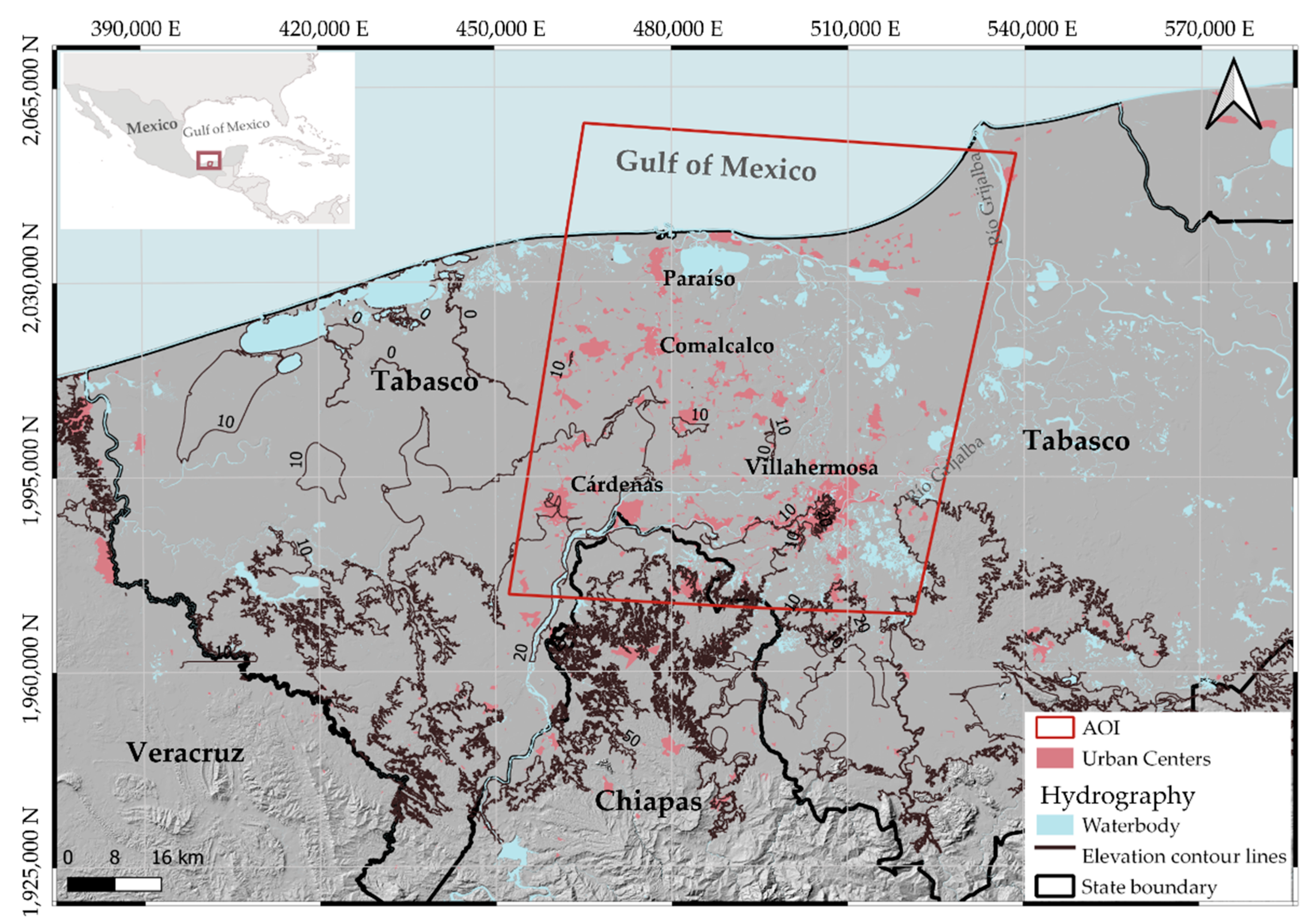
Figure 4.
Temporal and spatial (perpendicular) baseline connection diagram of the Sentinel-1 SLC image pairs from (a) ascending and (b) descending orbital pass used in the DIS approach.
Figure 4.
Temporal and spatial (perpendicular) baseline connection diagram of the Sentinel-1 SLC image pairs from (a) ascending and (b) descending orbital pass used in the DIS approach.
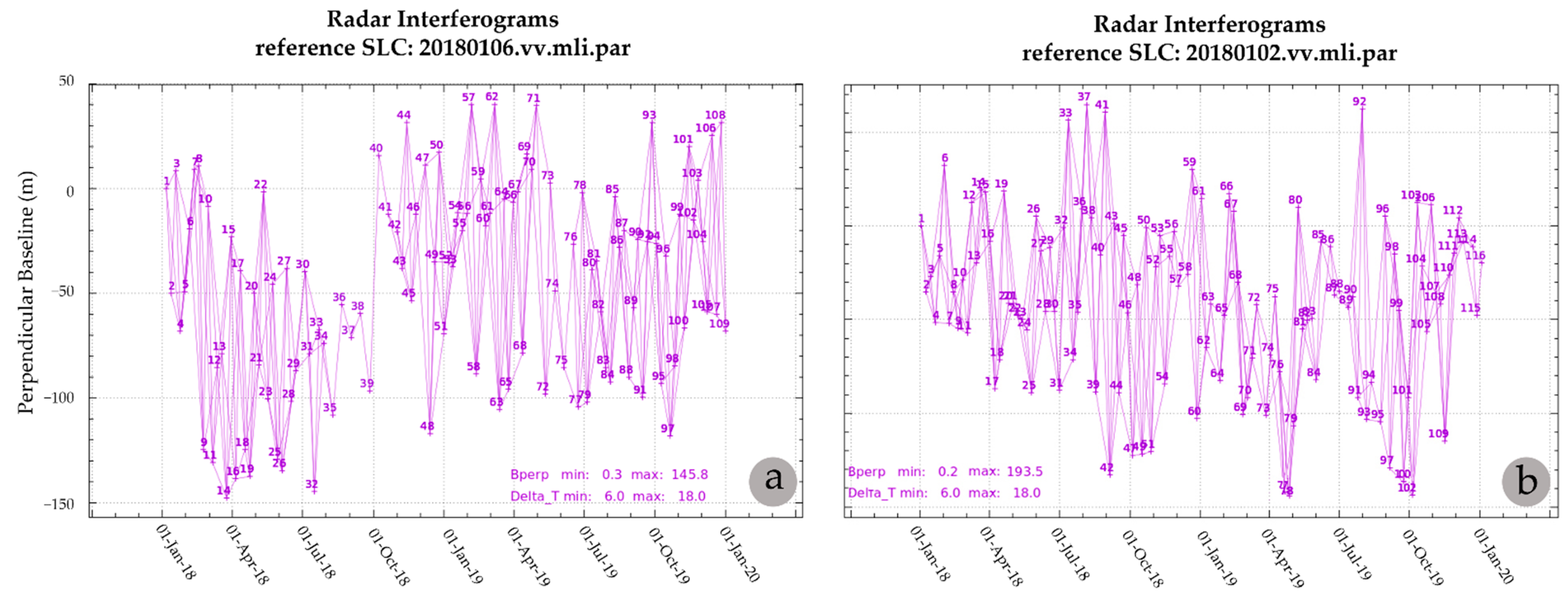
Figure 5.
(a) Coherence and (b) wrapped differential interferograms for selected Sentinel-1 SLC image pairs (Table 3).
Figure 5.
(a) Coherence and (b) wrapped differential interferograms for selected Sentinel-1 SLC image pairs (Table 3).
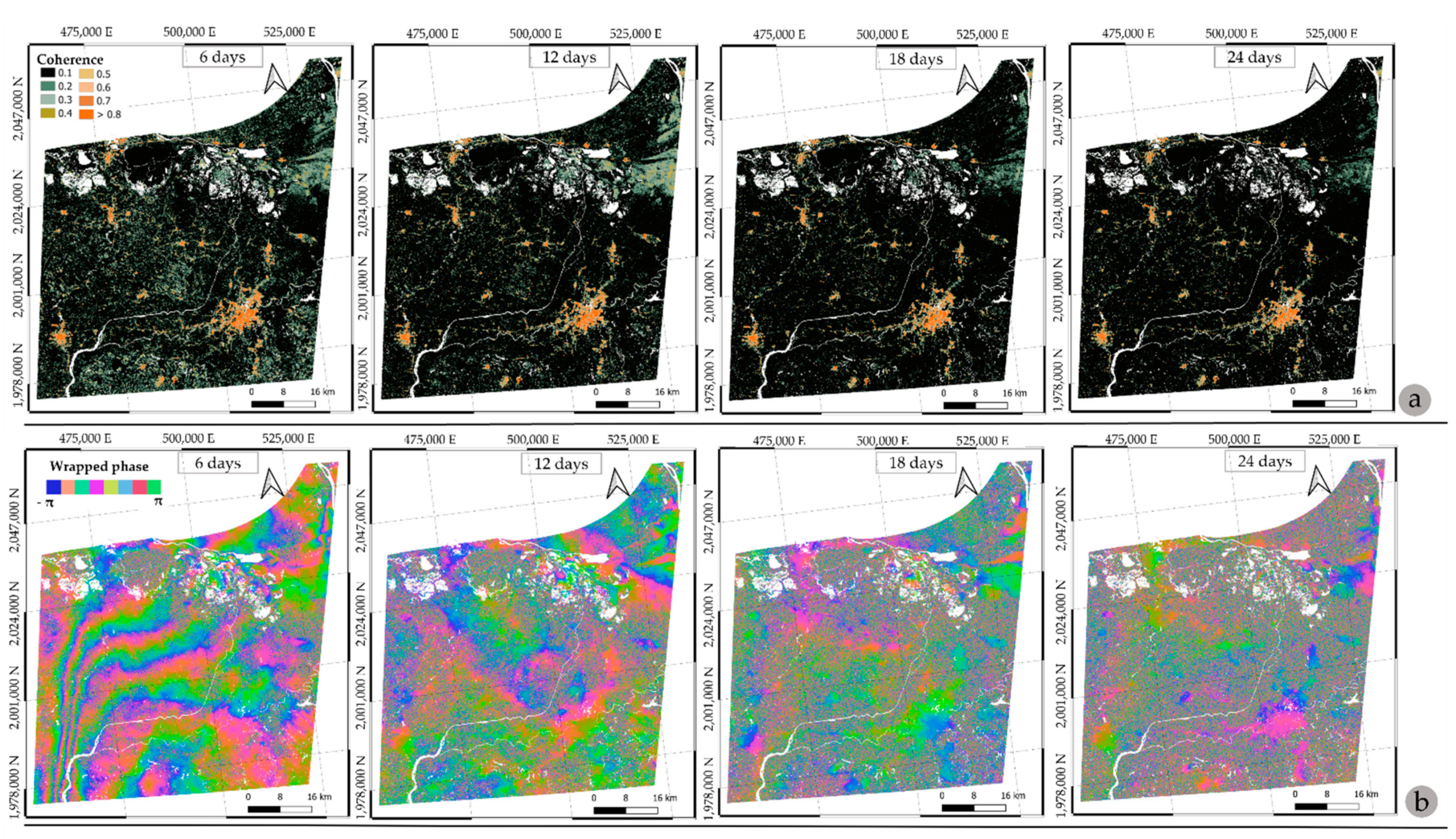
Figure 6.
Coherence histograms for selected Sentinel-1 SLC image pairs (Table 3). Arrows indicate the mean coherence value.
Figure 6.
Coherence histograms for selected Sentinel-1 SLC image pairs (Table 3). Arrows indicate the mean coherence value.

Figure 7.
Average coherence estimated for the 2018–2019 period using image pairs from the (a) ascending and (b) descending pass; (c) coherence histograms for each average coherence. Arrows indicate the mean coherence value.
Figure 7.
Average coherence estimated for the 2018–2019 period using image pairs from the (a) ascending and (b) descending pass; (c) coherence histograms for each average coherence. Arrows indicate the mean coherence value.
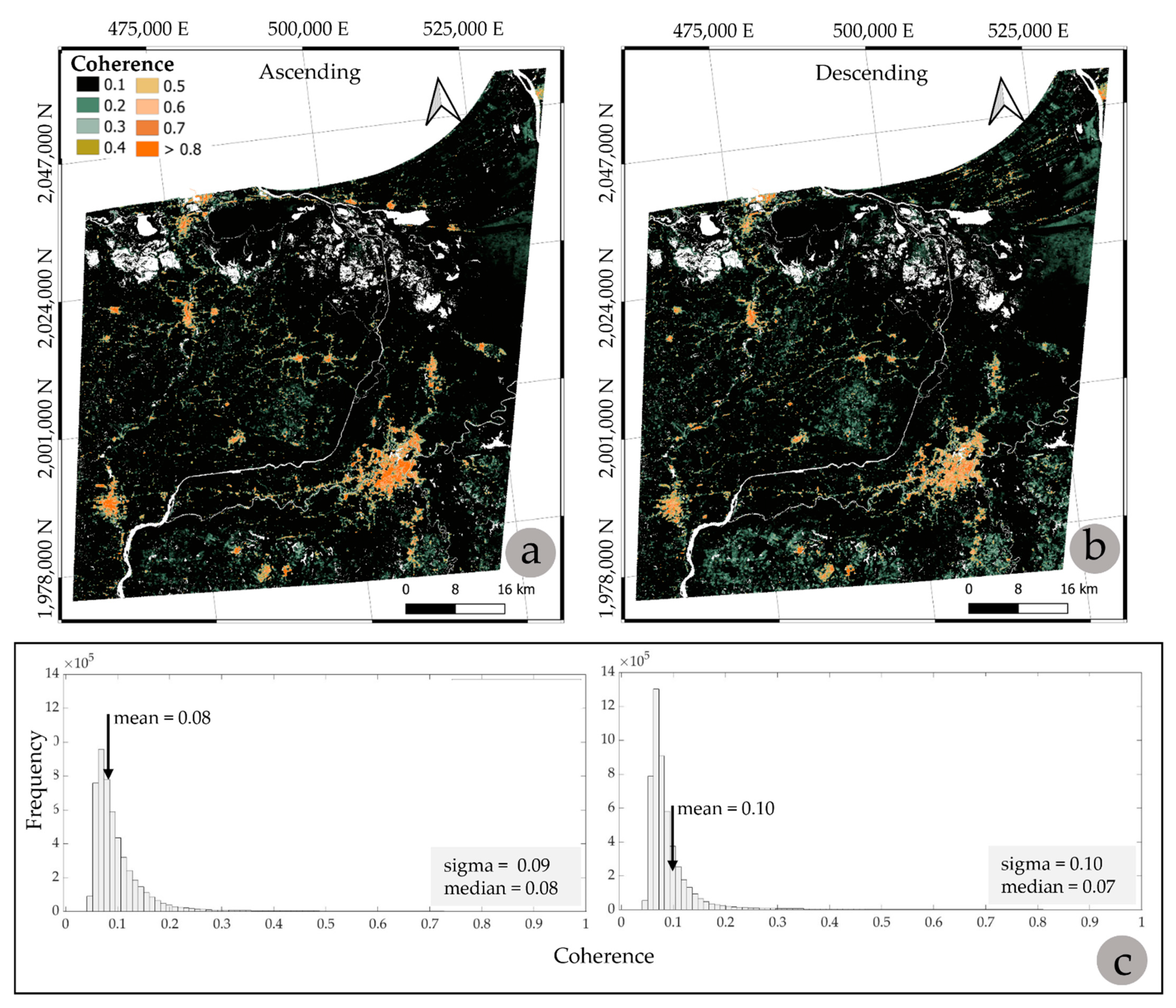
Figure 8.
Average coherence for different land cover classes, estimated for image pairs obtained from the descending orbital pass during the 2018–2019 period.
Figure 8.
Average coherence for different land cover classes, estimated for image pairs obtained from the descending orbital pass during the 2018–2019 period.
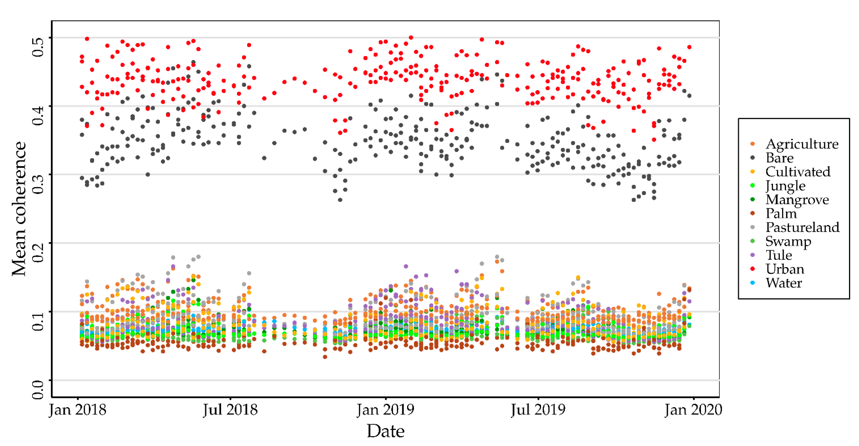
Figure 9.
Wrapped differential interferograms: (a) 14 December 2018–20 December 2018 and (b) 14 November 2018–20 November 2018; their respective coherence images (c,d), and histograms (e).
Figure 9.
Wrapped differential interferograms: (a) 14 December 2018–20 December 2018 and (b) 14 November 2018–20 November 2018; their respective coherence images (c,d), and histograms (e).
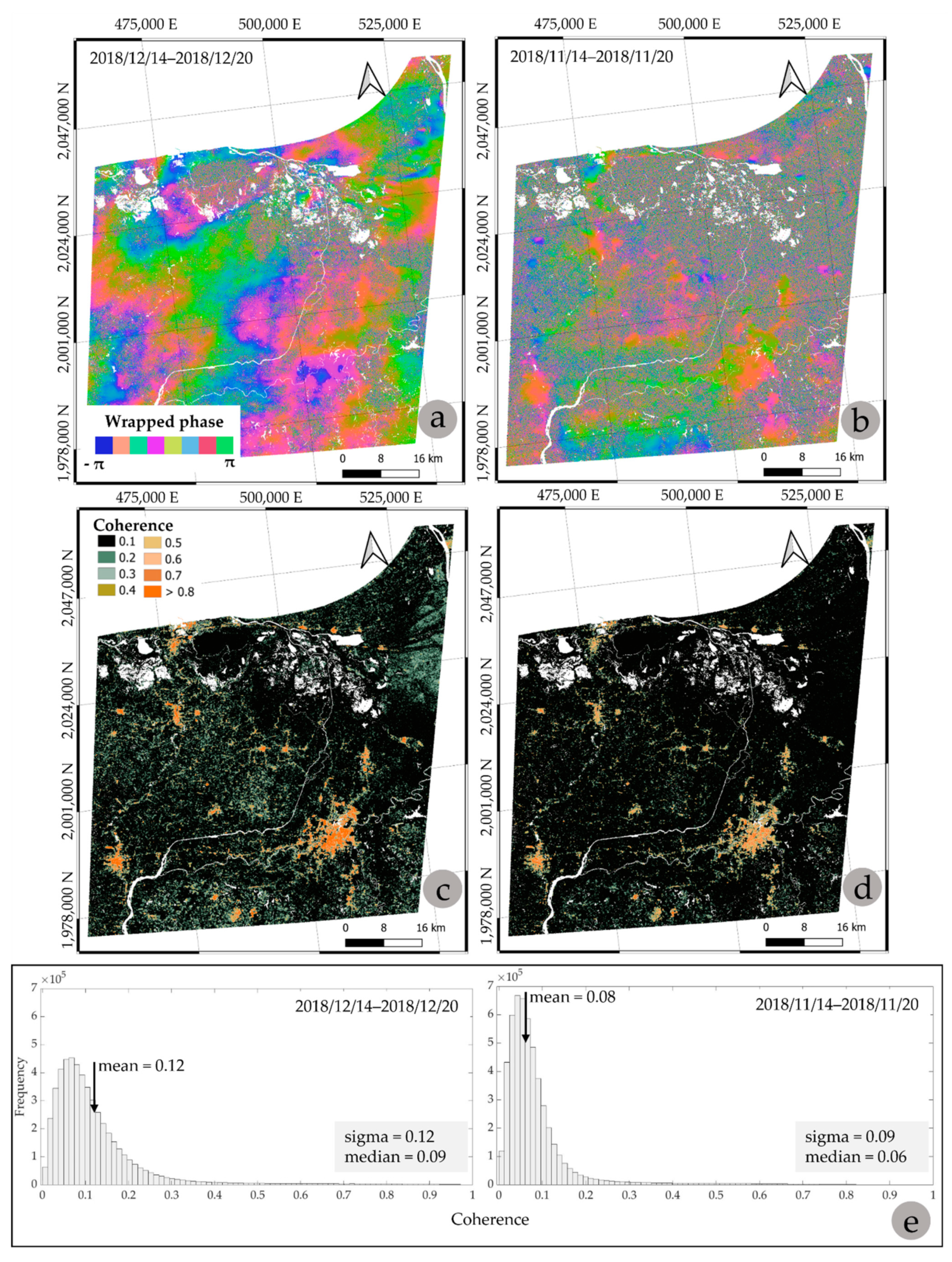
Figure 10.
Sentinel-1 GRD intensity (in dB) of (a) 6 January 2018, (b) 5 February 2018, (c) 16 October 2019, and (d) 21 November 2019. (a,c) Correspond to the images before the flood event, and (b,d) to the images during the floods.
Figure 10.
Sentinel-1 GRD intensity (in dB) of (a) 6 January 2018, (b) 5 February 2018, (c) 16 October 2019, and (d) 21 November 2019. (a,c) Correspond to the images before the flood event, and (b,d) to the images during the floods.

Figure 11.
Areas affected by the flood events of (a) 5 February 2018 and (b) 21 November 2019. Permanent water bodies are shown. A digital globe image is used as a background, the background image was taken from QGIS XYZ Tiles (https://mt1.google.com/vt/, accessed on 8 August 2022).
Figure 11.
Areas affected by the flood events of (a) 5 February 2018 and (b) 21 November 2019. Permanent water bodies are shown. A digital globe image is used as a background, the background image was taken from QGIS XYZ Tiles (https://mt1.google.com/vt/, accessed on 8 August 2022).
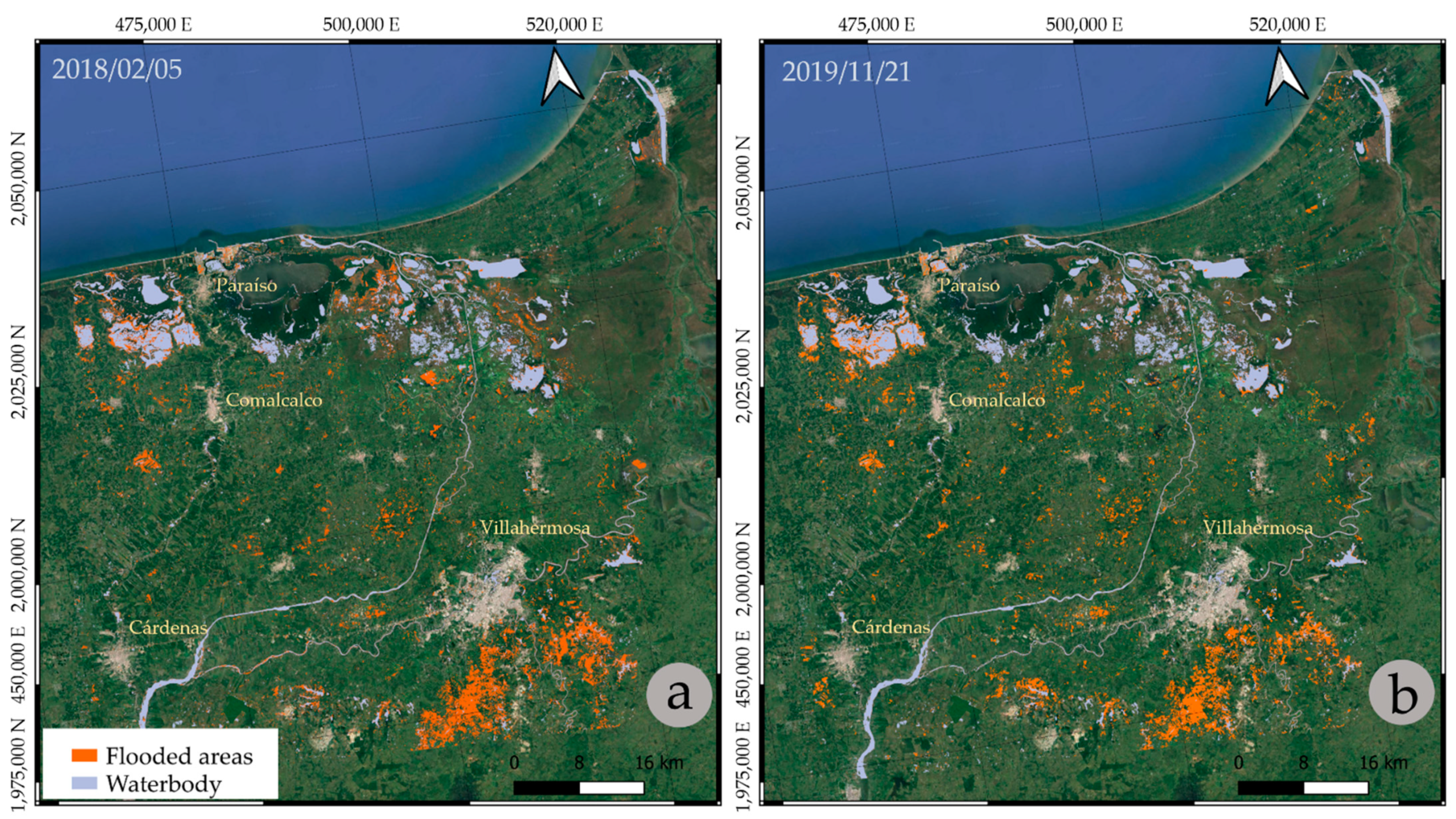
Figure 12.
Map of average LOS displacement rates (cm/yr) obtained through the DIS approach, using the Sentinel-1 SLC images of ascending orbital pass acquired in the 2018–2019 period. Negative values indicate a movement away the satellite, (a) full AOI map. Blue rectangles enclose the zones with a higher average LOS displacement rate. Close-ups of the (b) Paraíso and Comalcalco; (c) Villahermosa; (d) Batería Samaria and (e) Batería Cactus zones are presented. The location of hydrocarbon wells is also shown.

Figure 13.
Map of the average LOS displacement rate (cm/yr) obtained through the DIS approach using the Sentinel-1 SLC images of the descending orbital pass acquired in 2018–2019 period. Negative values indicate a movement away the satellite. (a) Full AOI map. Blue rectangles enclose the zones with a higher average LOS displacement rate. Close-ups of the (b) Paraíso and Comalcalco, (c) Villahermosa, (d) Batería Samaria and (e) Batería Cactus zones are presented. The location of hydrocarbon wells is also shown.


Table 1.
Characteristics of the Sentinel-1 SLC data used in this study in DInSAR processing. The nominal spatial resolution is specified for single-look data. N is the number of used SAR images, and I is the number of interferograms for each dataset calculated and analyzed in this study.
Table 1.
Characteristics of the Sentinel-1 SLC data used in this study in DInSAR processing. The nominal spatial resolution is specified for single-look data. N is the number of used SAR images, and I is the number of interferograms for each dataset calculated and analyzed in this study.
| Dataset | 1 | 2 |
|---|---|---|
| Orbit | Descending | Ascending |
| Mode | IW | IW |
| Sub-Swath | IW3 | IW2 + IW3 |
| Track | 99 | 34 |
| Frame | 530/532 | 54/55 |
| Wavelength (cm) | 5.5 (C-band) | 5.5 (C-band) |
| Polarization | VV | VV |
| Nominal ground resolution (Ground Range × Azimuth, m) | 5 × 20 | 5 × 20 |
| Time span | 2 January 2018–29 December 2019 | 6 January 2018–27 December 2019 |
| Number of images (N) | 115 | 108 |
| Number of Interferometric Pairs (I) | 321 | 290 |
Table 2.
Characteristics of the Sentinel-1 GRD data used to identify flooded areas.
| Image | Date | Format-Mode | Polarization | Land Surface Condition |
|---|---|---|---|---|
| 1 | 6 January 2018 | GRD-IW | VV | Dry |
| 2 | 5 February 2018 | GRD-IW | VV | Wet |
| 3 | 16 October 2019 | GRD-IW | VV | Dry |
| 4 | 21 November 2019 | GRD-IW | VV | Wet |
Table 3.
Parameters of image pairs selected for interferometric coherence analysis. Bp is the perpendicular baseline; Bt is the temporal baseline.
Table 3.
Parameters of image pairs selected for interferometric coherence analysis. Bp is the perpendicular baseline; Bt is the temporal baseline.
| Interferometric Pair | Orbital Pass | Bp (m) | Bt (Days) | Mean Coherence |
|---|---|---|---|---|
| 12 February 2019–18 February 2019 | Descending | 93 | 6 | 0.13 |
| 12 February 2019–24 February 2019 | Descending | 70 | 12 | 0.11 |
| 12 February 2019–02 March 2019 | Descending | 76 | 18 | 0.09 |
| 12 February 2019–08 March 2019 | Descending | 80 | 24 | 0.08 |
Table 4.
Parameters of interferometric pairs selected for the flood impact on the coherence degradation analysis. Bp is the perpendicular baseline; Bt is the temporal baseline.
Table 4.
Parameters of interferometric pairs selected for the flood impact on the coherence degradation analysis. Bp is the perpendicular baseline; Bt is the temporal baseline.
| Interferometric Pair | Orbital Pass | Bp (m) | Bt (Days) | Mean Coherence | Conditions |
|---|---|---|---|---|---|
| 14 November 2018–20 November 2018 | Descending | −85 | 6 | 0.08 | Wet (flood) |
| 14 December 2018–20 December 2018 | Descending | 82 | 6 | 0.12 | Dry |
Publisher’s Note: MDPI stays neutral with regard to jurisdictional claims in published maps and institutional affiliations. |
© 2022 by the authors. Licensee MDPI, Basel, Switzerland. This article is an open access article distributed under the terms and conditions of the Creative Commons Attribution (CC BY) license (https://creativecommons.org/licenses/by/4.0/).
Share and Cite
MDPI and ACS Style
Pérez-Falls, Z.; Martínez-Flores, G.; Sarychikhina, O. Land Subsidence Detection in the Coastal Plain of Tabasco, Mexico Using Differential SAR Interferometry. Land 2022, 11, 1473. https://doi.org/10.3390/land11091473
AMA Style
Pérez-Falls Z, Martínez-Flores G, Sarychikhina O. Land Subsidence Detection in the Coastal Plain of Tabasco, Mexico Using Differential SAR Interferometry. Land. 2022; 11(9):1473. https://doi.org/10.3390/land11091473
Chicago/Turabian StylePérez-Falls, Zenia, Guillermo Martínez-Flores, and Olga Sarychikhina. 2022. "Land Subsidence Detection in the Coastal Plain of Tabasco, Mexico Using Differential SAR Interferometry" Land 11, no. 9: 1473. https://doi.org/10.3390/land11091473
Note that from the first issue of 2016, this journal uses article numbers instead of page numbers. See further details here.