
Spatiotemporal Evolution Trends of Urban Total Factor Carbon Efficiency under the Dual-Carbon Background


School of Economics and Finance, Xi’an Jiaotong University, Xi’an 710061, China
*
Author to whom correspondence should be addressed.
Land 2023, 12(1), 69; https://doi.org/10.3390/land12010069
Submission received: 25 October 2022
/
Revised: 17 December 2022
/
Accepted: 21 December 2022
/
Published: 26 December 2022
(This article belongs to the Special Issue Urban Planning Pathways to Carbon Neutrality)
Abstract
:In order to grasp the development laws of carbon efficiency and help China to achieve the dual-carbon goal as soon as possible, we used the super-efficiency EBM model to calculate the total factor carbon efficiency of cities, based on panel data for 283 prefecture-level cities in China from 2004 to 2019. The spatiotemporal variations in carbon efficiency were analyzed using the Dagum Gini coefficient, LISA aggregation and standard deviational ellipse. The dynamic evolution trends were analyzed using kernel density estimation and the spatial Markov chain. The results showed that the overall difference in total factor carbon efficiency between the 283 cities decreased, and the difference within the three regions was greater than that between regions. The total factor carbon efficiency of the cities had a significant spatial correlation, and the spatial distribution patterns showed a centripetal aggregation from northeast to southwest. The dynamic evolution characteristics of the carbon emission intensity in different regions were quite different and the polarization of eastern and central cities was more obvious. There was a significant path dependence effect on the transition probability of total factor carbon efficiency between cities, and the carbon efficiency level of neighboring cities could affect the transition probability of the carbon efficiency of the cities. Based on the above conclusions, we also put forward relevant policy recommendations for technological changes on the energy supply side, innovative development patterns and the governance of regional policies.
1. Introduction
Across the world, in recent years, extreme climate events have occurred frequently, and global warming has been increasing. Ecological and environmental issues have become severe challenges to be addressed by all countries and countries are facing the increasingly urgent task of emission reduction. According to the Global Risks Report released by the Global Economic Forum in Davos in 2022, the top three risks are environmental issues. Of these, “poor climate action” was identified as the biggest risk facing the world over the next 10 years. In recent years, China has faced a number of development problems, such as insufficient energy and resource supplies, low energy use efficiency and the continuous deterioration of the ecological environment. The insufficient resource and environmental carrying capacity has become a bottleneck restricting China’s high-quality economic development. As the current largest energy consumer and greenhouse gas emitter, China has adopted the attitude of a responsible major country in global climate negotiations and has promised to implement more favorable policies and measures for environmental governance, strive to peak carbon emissions by 2030 and endeavor to achieve carbon neutrality by 2060. Nevertheless, even as the second largest economy in the world, China is still the largest developing country. Therefore, at this stage, the primary task is still to develop the economy. Coordinating the relationship between economic development and emission reduction has become a dilemma that every large developing country must face [1]. Improving carbon emission efficiency to minimize resource and environmental constraints, reducing energy dependence on fossil fuels and high-carbon industries and promoting green and low-carbon transformations are important strategies for achieving the dual-carbon goal. These strategies are also key to boosting high-quality economic development. China has a vast territory and there are huge differences in factor endowments, energy structures and technology levels between the regions, which leads to large differences in total factor carbon efficiency (TFCE) between the regions. In this context, the scientific and objective evaluation of TFCE and the analysis of its spatiotemporal differentiation and dynamic evolution trends could not only provide a systematic and comprehensive understanding of the development of China’s carbon efficiency level but also enable the central and local governments to grasp the development trends of TFCE in various regions in a timely manner. In turn, this could facilitate the formulation of various policies and measures related to carbon reduction and the reasonable allocation of energy-saving tasks so as to achieve the coordinated and overall development of regional carbon emission efficiency and lay solid foundations for the realization of the dual-carbon goal.
This work is arranged as follows: the second part is the literature review, sorting out the existing related literature, and then concluding the gaps in the existing literature and the innovation of this paper; the third part discusses the measurement method and variable selection of urban TFCE; the fourth part analyzes the spatiotemporal differentiation characteristics of TFCE; the fifth part studies the dynamic evolution trend of urban TFCE; and the last section summarizes the research conclusions and provides relevant policy suggestions accordingly.
2. Literature Review
2.1. Carbon Efficiency and Its Measurement Method
Driven by the dual-carbon goal, research on carbon emission efficiency has become an increasingly hot topic in academic circles. The origins of carbon emission efficiency can be traced back to the concept of carbon productivity, which was proposed by Kaya and Yokobori [2]. Nevertheless, carbon productivity does not consider the interactions between production input factors and cannot reflect the multidimensional characteristics of carbon emission efficiency in terms of economic production. The essence of carbon emission rates is to consider the technical production efficiency of carbon emissions [3]. therefore, carbon emission rates can be understood as obtaining more outputs with the same or fewer carbon emissions by considering the interactions between various input factors, such as capital and labor [4]. As a key part of China’s carbon peak and neutrality goals, the scientific and comprehensive measurement of carbon efficiency plays a crucial role in subsequent related research.
In terms of the measurement and evaluation of carbon efficiency indicators, existing studies have mainly involved single factor efficiency and total factor efficiency, among which the measurement of single factors refers to carbon emissions and the proportions of certain input factors; for example, the ratio of carbon emissions to GDP is used to measure carbon efficiency [5]. The measurement of total factor carbon efficiency usually involves the stochastic frontier analysis (SFA) method and the data envelopment analysis (DEA) method. Herrala et al. used the SFA method to measure the carbon efficiency of 170 pairs of countries in the world and found that there are huge differences in carbon efficiency levels and efficiency changes between the countries [6]. Du and Zou [7] and Chen and Huang [8] used the SFA method to calculate China’s provincial carbon efficiency. Because the SFA method needs specific settings on functional forms and has very strict assumptions, Charnes et al. proposed a non-parametric analysis method, namely the DEA method, which can not only take into account various input and output indicators, such as the economy and the environment, but can also effectively avoid the problem of subjective parameter weighting without setting specific function forms [9]. The International Energy Agency (IEA) measures carbon emission efficiency in different countries at the industrial level using the DEA method [10]. Ramanathan used the DEA model to calculate carbon emission efficiency at the national level and explored the factors affecting carbon emissions [11]. Nonetheless, the early DEA model required the input and output variables to be reduced in the same proportion, which is inconsistent with actual economic development and the radial model cannot measure non-radial relaxation variables [12]. Based on the above deficiencies, Tone introduced slack input and output variables into the objective function and constructed the non-radial SBM (slack-based measure) model [12], which effectively avoids the strict assumption that the factor inputs and outputs are reduced in the same proportion and can also incorporate undesirable outputs into the efficiency measurement process. Therefore, this method has become widely used in the measurement of carbon emission efficiency. Sun et al. used the SBM-DEA model to measure carbon efficiency levels [13]. Some scholars have also used the super-efficiency DEA model to measure and analyze inter-provincial carbon efficiency [14,15], industrial carbon emission efficiency [16], the carbon emission trading pilot market [17] and the carbon efficiency of the Yangtze and Yellow River basins in China [18].
2.2. Regional Differences in Carbon Emissions and Carbon Efficiency
Some Chinese scholars have analyzed the dynamic evolution characteristics of carbon efficiency and carbon intensity from the perspectives of regional differences and convergence. Zhou and Song measured the industrial carbon efficiency of China and concluded that industrial carbon efficiency has been increasing and that there are significant regional differences [19]. Lin et al. studied the spatiotemporal evolution characteristics of industrial carbon efficiency in the Beijing–Tianjin–Hebei region using kernel density estimation. Their empirical tests showed that there are large differences in carbon efficiency between industries and small differences between cities [16]. Jiang et al. analyzed the spatiotemporal evolution characteristics of carbon efficiency in the Yangtze River and Yellow River basins and concluded that carbon efficiency in this region shows the distribution characteristics of high in the middle and low at both ends and that the regions with high values form clusters [18]. Wang et al. and Han et al. used Theil Index to analyze the regional differences of China’s provincial carbon emissions and carbon productivity, respectively. The former study concluded that the gap of China’s provincial carbon emissions was expanding year by year [20], while the latter concluded that the regional differences of provincial carbon productivity were large [21]. Zhang et al. analyzed China’s carbon emission intensity using kernel density estimation and concluded that carbon intensity shows a distribution pattern of “low in the south and high in the north”, with significant differences in dynamic evolution between different regions. Significant β convergence was observed in the carbon intensity of the whole country and major strategic regions [22].
2.3. The Gaps in the Existing Literature and the Innovation of This Paper
In general, the existing research on the connotations, extension and quantitative measurement of carbon efficiency has achieved certain results, which have laid the foundations for subsequent related research. However, there are also some shortcomings. Firstly, the existing research on carbon efficiency has mainly focused on the macro level, such as national, provincial and industrial levels. Due to the limitations of data acquisition, relevant research on TFCE at the urban level in China is still lacking. Secondly, research on the spatial distribution of carbon efficiency is still in its infancy and the overall research is still relatively rough. There have been few studies on the spatiotemporal differentiation and dynamic evolution of urban TFCE, which is not conducive to the overall improvement of China’s carbon efficiency and coordinated development between regions. Thirdly, in terms of the measurement and evaluation of carbon efficiency, most of the existing studies have used the super-efficiency SBM-DEA model for their calculations; however, the SBM model cannot provide the ratio information between the actual value of the input (output) index and the target value [23], which can lead to deviations in measurement results. Fourth, most of the existing studies have used Theil index and the kernel density estimation method to reveal the regional differences and dynamic evolution characteristics of the research objects, and few have used the Dagum Gini coefficient and standard deviational ellipse method to analyze carbon efficiency. The standard deviational ellipse and the center of gravity transfer analysis can intuitively reveal the various spatial characteristics of TFCE. They can also complement the Dagum Gini coefficient decomposition method and kernel density estimation method. Fifth, the existing research has paid attention to the spatial distribution of carbon emissions and carbon efficiency but has not analyzed the spatiotemporal transfer probability of carbon efficiency. Additionally, there have been even fewer relevant studies on urban TFCE.
The innovations of this paper are as follows. In terms of research object, this study focused on the city level, took panel data for 283 prefecture-level cities in China as samples and calculated urban carbon emissions by combining the energy consumption generated by major carbon emission sources (i.e., the consumption of electricity, liquefied gas, liquefied petroleum gas and thermal energy in the whole society) with their respective carbon emission coefficients. Then, the super-efficiency EBM model with radial mixing parameters was combined with the GML index to calculate TFCE at the city level. In terms of the research method, the Dagum Gini coefficient, Moran’s I index, a LISA aggregation map and the standard deviational ellipse method were used to comprehensively analyze the regional differences in the distribution and spatiotemporal differentiation characteristics of TFCE. Then, kernel density estimation and the spatial Markov chain method were used to analyze the development status and spatiotemporal evolution characteristics of TFCE at the city level. The obtained conclusions are not only conducive to a comprehensive and systematic understanding of the development of TFCE at the city level in China but could also provide useful references for local governments to help them to formulate relevant strategies for the coordinated development of regional carbon efficiency.
3. Measurement of Urban TFCE
3.1. Method of Measurement
3.1.1. Super-Efficiency EBM Model
In order to effectively make up for the shortcomings in efficiency measurement using the CER and SBM models, Tone et al. constructed a model that includes both radial and SBM distance functions, namely the epsilon-based measure (EBM) model [24]. The super-efficiency EBM model relaxes the assumption regarding the proportion between the target value and the actual value of the input and can also calculate the difference between the target value and the actual value by solving the non-radial values of the input and output variables. Therefore, the efficiency value of the obtained decision-making unit (DMU) is more accurate [25]. In this study, we selected the super-efficiency EBM model to define the directional distance function (DDF), which was set as the global super-efficiency, non-orientation and variable returns to scale to measure TFCE at the city level in China [26]. The global super-efficiency EBM model was constructed as follows:
In the above formula, γ* is the TFCE value; n is the number of DMUs j; x is the input factor; y is the desirable output; u is the undesirable output; m, k and h represent the quantities of input factors, desirable outputs and undesired outputs, respectively; θ is the planning parameter of the radial part; η is the output expansion ratio; ε is the parameter referring to the importance of the non-radial part, where 0 ≤ εx ≤ 1; , and are the weights of the i-th input, r-th expected output and p-th unexpected output, respectively; and , and are the relaxation variables of the i-th input, r-th desirable output and p-th undesirable output, respectively.
3.1.2. Global Malmquist Index
In 1953, the Swedish economist Malmquist proposed the Malmquist (ML) index [27], which can measure the dynamic rate of change of DMUs using the distance function. However, this index does not have circularity, nor can it analyze the rate of change of the efficiency of technical progress over set periods [28]. Additionally, the ML index may have the problem of no linear solutions in the calculation process. The Global Malmquist (GML) index calculates global production possibility sets based on data from all sample periods, which can effectively solve these problems of non-transmission and no linear solutions. The GML index can be decomposed into the rate of change of technical progress (GETC) and the rate of change of technical efficiency (GEFC) [29]. Since the super-efficiency EBM model adopted in this study could only provide static efficiency values, it was necessary to measure and decompose China’s city-level TFCE dynamically using the GML index. The expression of the GML index is as follows:
In Formula (3), xt, yt and ut and xt+1, yt+1 and ut+1 represent the input, desirable output and undesirable output of DMUs in the t and t+1 periods, respectively, and DG(xt, yt, ut) is the mixed distance function of the EBM model. The calculation method of this function is shown in Formula (1).
3.2. Index Selection and Data Processing
The input indicators of TFCE at the city level were defined as follows: human capital, measured by the number of employees in the selected three industries in each city; capital stock, for which the fixed capital investment flow data were deflated by the fixed asset price index after eliminating the price factor and subtracting the accumulated depreciation and the actual fixed capital stock was calculated using the perpetual inventory method; energy consumption, measured by the total energy consumption of each city. The output indicators of TFCE at the city level were defined as follows: the desirable output was measured by the actual GDP of each city; the undesirable output was the CO2 emissions of each city. The measurement of carbon emissions at the city level in existing studies has mainly involved carbon emissions from electricity production, natural gas, liquefied petroleum gas (LPG), urban heating and transportation [30], among which the carbon emissions generated by power production account for nearly half of China’s total carbon emissions [31] while urban heating, natural gas and LPG generate the next highest amounts of carbon emissions. Furthermore, the carbon emissions generated by transportation account for a small proportion of the total carbon emissions of each city [32] and the transportation carbon emission data at the city level are incomplete, so this indicator was removed from our measurement. Therefore, we referred to the method of Wu and Guo [33] for the measurement of carbon emissions in prefecture-level cities and selected four types of energy consumption for calculation: electricity consumption, liquefied gas consumption, LPG consumption and thermal energy consumption. The formula for the measurement of carbon emissions at the city level is as follows:
In Formula (4), Cm, Cn and Cp represent the carbon emissions generated by liquefied gas, LPG and urban heating, respectively; Em, En and Ep represent natural gas consumption, LPG consumption and urban heating consumption, respectively; γ, λ and τ are the carbon emission coefficients of the three energy types1; Cq represents the carbon emissions generated by urban electricity use, where Cq = φ(η × Eq), according to the research of Glaeser and Kahn [34]. The power grid in China is divided into six regions: South China, East China, Central China, North China, Northeast China and Northwest China. Each region has an emission factor and φ is the emission factor generated by electric energy consumption in each region, η represents the ratio of coal power generation to total power generation and Eq represents the electricity consumption of the whole society.
In this study, we selected panel data for 283 cities in China from 2004 to 2019 and used MAX-DEA software to calculate the TFCE. The data used for the variables came from the China Statistical Yearbook, China Urban Statistical Yearbook, China Power Yearbook, China Labor Statistical Yearbook, WIND database, CEIC database, etc.
4. The Spatiotemporal Differentiation Characteristics of Urban TFCE
4.1. Research Methods
4.1.1. Dagum Gini Coefficient and Decomposition Method
We used the Dagum Gini coefficient (G) and its decomposition method to explore the relative spatial differences in TFCE at the city level. Dagum decomposed the Gini coefficient into three components: within-group differential contribution (Gw), between-group differential contribution (Gnb) and hypervariable density contribution (Gt) [35]. The relationship between the Gini coefficient and its decomposition term is G = Gw + Gnb + Gt. In this paper, Gw represents the difference in TFCE value added between cities in different regions of China, Gnb represents the difference in TFCE value added between cities in the eastern, central and western regions of China and Gt is the remainder of the cross-influence of the Gini coefficient between the three regions. A smaller within-group Gini coefficient (between-group) indicates a smaller TFCE difference between within-group cities (between-group) and larger coefficients indicate larger differences. The Dagum Gini coefficient is calculated as follows:
In Formula (5), k represents the number of regions; j and h represent different regions; n represents the number of cities; i and r represent different cities; nj(nh) represents the number of cities in region j(h); yji (yhr) represents the TFCE of city i(r) in region j(h); μ is the mean growth of TFCE in all cities in the four regions; Gjj is the Gini coefficient of region j; Gjh is the Gini coefficient between region j and h; Gw is the within-group difference contribution; Gnb is the between-group difference contribution; and Gt is the hypervariable density contribution after Dagum Gini coefficient decomposition. These terms are calculated as follows:
In the above formulae, , and Djh represents the interaction effect of TFCE between regions j and h. The calculation method for the difference is shown in Equation (13). Additionally, djh is the difference in TFCE between regions, representing the mathematical expectation of all yji − yhr > 0 in regions j and h; pjh is the hypervariable first-order matrix, representing the mathematical expectation of all yhr − yji > 0 in regions j and h; and Fj(Fh) is the cumulative density distribution function of region j (h).
4.1.2. Global Spatial Correlation Test
In order to investigate whether there was spatial dependence in the data, it was necessary to conduct a spatial correlation test on the urban TFCE. The Moran’s I index was used to test the global spatial correlation of TFCE at the city level and the selected spatial weight matrix was the geographical distance weight matrix. The formula for the global spatial autocorrelation is as follows:
In the above formula, i and j represent different cities, n represents the number of cities, Y represents the TFCE of the city, represents the mean TFCE value of the city and Wij represents the spatial weight matrix. A Moran’s I∈[−1, 1] value greater than 0 represents positive autocorrelation, a Moran’s I∈[−1, 1] value less than 0 represents negative autocorrelation and a Moran’s I∈[−1, 1] value equal to 0 represents no correlation.
4.1.3. Local Spatial Autocorrelation
The local spatial autocorrelation mainly uses the local Moran index to observe the type of spatial agglomeration to which the spatial unit belongs [36]. In this study, the local spatial correlation index (LISA aggregation) was used to measure the local spatial correlation of urban TFCE. LISA aggregation maps can visually show the significance of the local spatial aggregation of urban TFCE in the form of graphs, as well as reflecting the specific spatial correlation forms of research elements in the aggregation maps at the same time. Our LISA aggregate graphs were generated based on the local Moran’s I index and the specific calculation formula was as follows:
In Formula (15), Moran’s Iit is the local Moran index and S2 is the variance. The other parameters were set to be the same as those in Formula (14). Similar to the global Moran index, the local Moran’s Iit ∈ [− 1, 1]. The LISA aggregation maps were generated by combining the scatter maps obtained using the Moran index with the significance of the LISA aggregation.
4.1.4. Standard Deviational Ellipse
The standard deviational ellipse method is a classical method that is used to analyze spatial distribution characteristics [37]. A standard deviational ellipse is composed of the center of a circle, the azimuth angle, the major axis, the minor axis and the ellipse area [38]. The center of a standard deviational ellipse represents the center of gravity for the spatial distribution of the elements and the azimuth angle represents the main spatial distribution trends of the research elements. The major and minor axes reflect the dispersion degree of the spatial layout of the research elements in the primary and secondary directions, respectively, while the area of the standard deviational ellipse reflects the aggregation and dispersion degree of the spatial distribution forms of the research elements. The calculation formulae for the standard deviational ellipse and its components are as follows:
In Formulae (16)–(20), and represent the weighted average center of the ellipse, xi and yi are the spatial coordinates of each feature point, and are the deviations of different feature points from the average center coordinates, wi is the weight, θ is the azimuth angle, σx and σy represent the standard deviations along the x and y axes of the ellipse, respectively.
4.2. Empirical Analysis
4.2.1. Analysis of the Dagum Gini Coefficient Results
Table 1 presents the Dagum Gini coefficients of TFCE at the city level and the decomposition results for the three regions. The results showed that the mean of the overall Gini coefficient in China was 0.0537 and that the change in the overall difference had an inverted “N” shape, i.e., During the sample period, the overall difference in TFCE between the cities tended to decline in the fluctuation. Specifically, the overall relative difference in urban TFCE during 2007–2015 was lower than the average level and decreased continuously, while the difference in urban TFCE during 2016–2019 first decreased and then increased. From the perspective of differences in change trends, the Gini coefficient decreased from 0.1025 in 2005 to 0.0538 in 2019, with a decrease rate of 47.51%, which meant that the difference in TFCE between cities in China as a whole decreased.
Additionally, from the perspective of intra-regional differences, among the three selected regions, the mean urban TFCE Gini coefficients in the eastern and western regions were lower than the national average, while the Gini coefficient in the central region was higher than the national average, which indicated that the intra-regional differences in urban TFCE were very significant. Specifically, the Gini coefficient in the eastern region showed an inverted “N”-shaped feature and the TFCE variation trends in the central and western cities were basically the same. During 2005–2015, the TFCE variation trend had a “W”-shaped pattern, with alternating decreases and increases. The variation trend during 2016–2019 had an “N”-shaped pattern, but the Gini coefficient in the central region was higher than those in the eastern and western regions as a whole. This indicated that the TFCE changes in the central and western cities were unstable, while the Gini coefficients in the eastern region showed stable changes in the early stages and significant fluctuations in the later stages.
Moreover, from the perspective of inter-regional differences, the variation trends in the relative differences between the three regions first decreased and then increased. The mean of the relative difference coefficient between the central, eastern and western regions was lower than the national average level, while the Gini coefficients between the eastern and central regions and the central and western regions were higher than the national average. Specifically, the relative difference between the eastern and central regions was the largest, followed by the difference between the central and western regions. The relative difference between the eastern and western regions was the smallest. In terms of stability trends, the relative difference coefficients between the three regions changed stably from 2007 to 2015 but fluctuated significantly after 2016.
From the perspective of contribution rates and the sources of differences, the contribution rate of regional differences in TFCE between 2005 and 2019 ranged from 30.38% to 33.39% and the contribution rate only changed slightly over time. The contribution rate of inter-regional differences had a large variation range, but its value was significantly smaller than the contribution rate within the regions, indicating that there were huge differences in total factor carbon efficiency between Chinese cities within the three regions and that the differences between regions were small. These differences led to significant differences in TFCE within the overall region of China, which means that in order to improve the overall TFCE level of Chinese cities, we should focus on the development gaps in each region. The contribution rate of hypervariable density showed a fluctuating trend from 2005 to 2019, during which time its value ranged between 45.77% and 64.56%. Under the influence of contribution rate, the intra-regional differences to the overall national difference ranged between 0.0111 and 0.0338 and decreased slightly over time. The inter-regional differences ranged between 0.0009 and 0.0133 and the change trend had an inverted “N” shape, with alternating decreases and increases. The interaction effect of intra-regional and inter-regional differences decreased slightly from 0.0621 at the beginning of the period to 0.0308 at the end of the period, with a decrease rate of 50.40%. In general, the intra-regional differences were higher than inter-regional differences and the hypervariable density was significantly higher than the intra-regional and inter-regional difference values, which meant that the interaction levels between intra-regional and inter-regional relative differences contributed the most to differences in urban TFCE, followed by intra-regional differences.
4.2.2. Global Spatial Correlation Test
The results of the urban TFCE global spatial correlation test are shown in Table 2. The Moran ‘I index values for urban TFCE were all greater than 0 and were all significant at the level of at least 1%, which confirmed that there was a significant positive spatial correlation between the TFCE of Chinese cities. This meant that the TFCE of each city was not completely independent or randomly distributed in space. This is because there is a cluster effect in economic production activities, through which the flow of production, technology and other factors make economic activities in neighboring cities converge, resulting in the spatial spillover effect of TFCE between cities. In addition, carbon emissions are inherently spatially dispersed, especially in geographically concentrated areas, which leads to the existence of spatial aggregation in urban TFCE.
4.2.3. LISA Aggregation Graphs
In order to show the spatial correlation effect of urban TFCE, ArcGIS software was used in this study to combine the local Moran index and the LISA significance level. Then, LISA aggregation maps were drawn for 2005, 2013 and 2019 as the representative years, as shown in Figure 12. LISA aggregation maps divide local spatial correlation into four types, namely, high–high (H-H) aggregation, high–low (H-L) aggregation, low–high (L-H) aggregation and low–low (L-L) aggregation. Among them, H-H aggregation and L-L aggregation indicate that there is a positive spatial correlation between the TFCE of a given city and the TFCE of other cities in the same agglomeration area. H-L aggregation and L-H aggregation indicate that there is a negative spatial correlation between the TFCE of a given city and the TFCE of other cities in the same agglomeration area.
As shown by the transfer trends of TFCE local spatial aggregation in Figure 1a–c, the H-H and L-L aggregation areas formed in the spatial correlation of urban TFCE changed greatly over time. Some cities located in H-H aggregation areas in 2005 were transformed into L-L aggregation areas in 2013 and then transformed back into H-H aggregation areas again in 2019, such as Yulin City and Luliang City. Some cities located in L-L aggregation areas in 2005 were transformed into spatially insignificant areas over time, such as Hegang, Jiamusi and Shuangyashan, while other cities located in L-L aggregation areas in 2013 were transformed into H-H aggregation areas in 2019, such as Jiuquan and Jiayuguan. In 2005 and 2013, fewer cities were located in H-L and L-H aggregation areas and the TFCE of these cities was negatively correlated with neighboring areas. For example, Zhangye and Tianshui, which were located in a H-L aggregation area, had high efficiency levels but inhibited the efficiency levels of their neighboring cities. However, other cities, such as Datong and Zhangjiakou, were located in L-H agglomeration areas, which indicated that the low efficiency levels of these cities did not inhibit TFCE in the surrounding areas but instead promoted it.
In general, compared to 2005 and 2013, the number of cities located in H-H and L-L aggregation areas increased in 2019 and these two areas formed a significant north–south differentiation feature in space. The high aggregation areas were mainly distributed in the northeast, northwest and north of China, such as Shenyang, Beijing, Tangshan and Jiuquan. These cities not only had higher TFCE levels but also had positive spillover effects on the carbon efficiency levels of surrounding cities through the positive diffusion effect. The L-L aggregation areas were mainly located to the south of the Qinling Mountains and the Huaihe River, such as Lishui, Nanchang and Lincang. The TFCE levels of these cities were low, which further inhibited TFCE improvements in surrounding cities and showed the agglomeration effect of inefficient cities in space.
The L-H agglomeration areas were mainly concentrated in the northeastern and northwestern regions, while the number of cities in H-L agglomeration areas was the lowest, indicating that there was a negative correlation between the TFCE of these cities and their neighboring regions and that the low (high) TFCE of one city could promote (inhibit) the TFCE of neighboring cities.
4.2.4. Standard Deviational Ellipse
Figure 2 shows a directional distribution map of urban TFCE based on the standard deviational ellipse, which was drawn using ArcGIS software. The obtained parameters are shown in Table 3. It can be seen from Figure 2 that the TFCE of Chinese cities was centered around Zhumadian City and that the dominant distribution direction extended from northeast to southwest. The barycentric coordinates of the ellipse presented in Table 3 were located between longitude 113°54′–113°93′ E and latitude 32°85′–33°14′ N and were slightly to the southeast of Lanzhou, which is the geographic and geometric center of China (longitude 103°40′ E and latitude 36°03′ N). From the perspective of the shifting trajectory of the center of gravity, the center of gravity of urban TFCE did not change significantly from 2005 to 2019, which meant that the TFCE in eastern and southern China was higher on average than that in other regions. This was consistent with the reality that China’s economic development is higher in the east than in the west. During the sample period, the azimuth angle of the ellipse ranged between 22° and 24° and increased slightly in 2019 compared to 2005, indicating that the divergence direction of the TFCE of Chinese cities was also relatively stable. The ratio of the minor axis to the major axis gradually decreased over time. The oblateness of the ellipse was the smallest in 2005 and the largest in 2019, i.e., the centripetal force of urban TFCE had an increasing trend from 2005 to 2019. In 2019, the directionality of the urban TFCE distribution was the most significant. As shown in Table 3, the ellipse area showed a fluctuating upward trend and the ellipse area in 2019 decreased by 4.61% compared to the area in 2005, indicating that the spatial aggregation degree of the TFCE of Chinese cities improved slightly. However, in general, this spatial aggregation characteristic was relatively stable during the sample period.
5. Dynamic Evolution Trend Analysis of Urban Total Factor Carbon Efficiency
5.1. Research Method
5.1.1. Kernel Density Estimation
Kernel density estimation is a non-parametric estimation method, which can describe the distribution characteristics of estimation variables well. This method has a low dependence on the model and has a strong robustness, so it is widely used in spatial disequilibrium analysis [39]. Therefore, in order to further explore the distribution differences and evolution rules of China’s urban TFCE at the national and regional levels, the kernel density estimation method was adopted to describe the distribution forms of TFCE at the city level using continuous changing curves so as to show the distribution location, form and characteristics of urban TFCE more comprehensively. Let f(z) be the density function of urban TFCE, then
In Formula (21), m is the number of observations, v is the bandwidth, K(∙) is the kernel density function, δi is the independently distributed observation value and is the mean of the observation values. In this study, the Gaussian kernel density function was selected to estimate the dynamic distribution of TFCE at the national and regional levels. Its formula is as follows:
Since there is no exact function expression for non-parametric estimation, it is necessary to observe distribution characteristics by means of graphical comparisons as graphs obtained by kernel density estimation can provide information about different dimensions, such as distribution position and shape and the ductility of the variables.
5.1.2. Spatial Markov Chain Method
Although kernel density curves can better describe the distribution characteristics and convergence degrees of variables, they offer limited internal dynamic information regarding variable distributions and fail to show the relative location change characteristics and future occurrence possibility of TFCE at the city level. The Markov chain method considers random variables as discrete variables, which can make up for these shortcomings. Therefore, we used the Markov chain method to describe the state transition of TFCE in each city, as well as the possibility of transition. A Markov chain is a stochastic process, namely {Xt, t∈T}, which describes the internal change probability of variables by constructing a Markov transition probability matrix [40]. Markov chains assume that the probability of state j, in which the variable X is in period t, is determined by the state in period t-1 and is independent of the other periods, i.e.:
In Equation (23), Pij is the transition probability matrix of TFCE in a given city from year t to year t+1. Based on a traditional Markov chain, the concept of “spatial lag” is introduced to obtain a spatial Markov chain. By introducing a spatial weight matrix (Wij), the transition probability matrix of N × N is decomposed into N × N × N so that Pij can reveal the evolution process of the spatial lag effect on urban TFCE. The spatial weight matrix Wij in this study was represented by a spatial adjacency matrix. The formula was as follows:
5.2. Analysis of the Urban TFCE Spatiotemporal Evolution Results
5.2.1. Analysis of Kernel Density Results
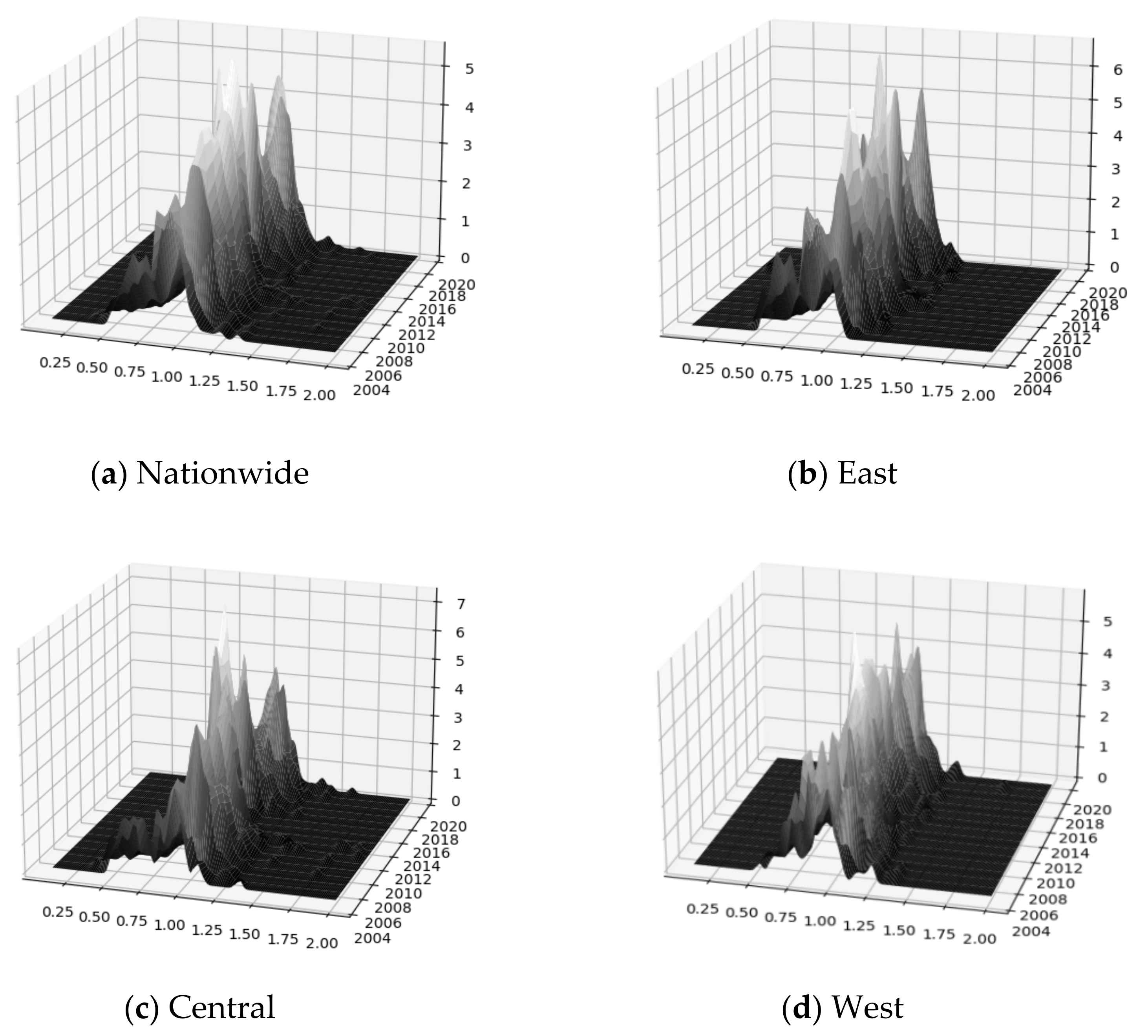
In order to systematically analyze the absolute distribution differences and dynamic evolution laws of urban TFCE, the Gaussian kernel function was selected to depict the distribution laws of TFCE and kernel density curves were drawn using Python 3.8 software. Figure 3 and Table 4 show the distribution dynamics and evolution trends of TFCE in the whole country and the three selected regions.
In terms of the whole country, the main peak position of urban TFCE showed a trend of right–left alternating movement during the investigation period. From 2018, the main peak gradually moved to the right, indicating that the overall TFCE of the whole country effectively improved during this period. This was mainly due to the influence of multiple factors, such as China’s green energy transformation and upgrade policies, green scientific and technological innovations and the continuous enhancement of the carbon absorption capacity of terrestrial ecosystems over recent years. In terms of the distribution pattern of the main peak, the height of the main peak first increased and then decreased, while the width of the main peak gradually decreased. As shown in Figure 3a, the height of the main peak in 2019 was higher than that in 2005 and the width narrowed, indicating that the absolute difference in domestic TFCE and the dispersion degree of the distribution both decreased. From the perspective of distribution ductility, the national TFCE distribution curve dragged to the right and showed the characteristics of extended convergence. The higher carbon efficiency levels of some cities led to a right-trailing distribution curve, while the convergence trend indicated that the difference between cities with high carbon efficiency levels and the average level across the country gradually decreased. From the perspective of the polarization trend, the overall TFCE of the country showed a trend of multipolar differentiation, i.e., there as a multipeak phenomenon in addition to the main peak. This was because although the TFCE of some cities showed overall growing trends, they were restricted by various factors, such as differences in energy and resource endowment, economic development and technological level. Therefore, the absolute differences between cities with higher TFCE levels and those with lower TFCE levels were characterized by fluctuating short-term changes.
In terms of the distribution locations and forms of the three selected regions, the positions of the main peaks of TFCE in the eastern and central regions alternated between shifting to the left and right while the position of the main peak in the western region gradually moved to the right, indicating that the TFCE levels in the eastern and central regions fluctuated and changed over time (and even decreased in some years) while the TFCE level in the western region gradually improved. The height of the main peak in the eastern region first increased and then decreased and the width gradually decreased, indicating that the dispersion of its distribution decreased and the absolute difference decreased further. The height of the main peak in the central region also first increased and then decreased and the width increased at the end of the period, which indicated that the dispersion degree and the absolute difference in the TFCE of the central region showed “V” shape patterns. The height of the main peak in the western region increased over time, indicating that the dispersion degree of the TFCE distribution decreased. The peak width also gradually decreased during the sample period, indicating that the absolute TFCE differences within the western region decreased.
From the perspective of distribution extensibility and polarization trends, the TFCE distribution curves for the three regions all trailed to the right and showed extended convergence, indicating that the difference between the cities with high TFCE levels and the average levels in the eastern, central and western regions gradually decreased. There were multiple main peaks in the distribution curves for the eastern and central regions, which showed that the multipolar differentiation in the TFCE levels of cities in the two regions was very significant, thereby confirming that there was also a significant differentiation between cities in the eastern and central regions. The western region showed a polarization trend, with a main peak and a left-hand peak in the early stages and the side peak gradually merging into the main peak in the middle stages, which evolved into a main peak and the polarization phenomenon gradually disappeared. A right-hand peak formed in the later stages.
5.2.2. Analysis of Spatial Markov Chain Results
In order to explore the dynamic evolution trends of urban TFCE levels in China, we used a traditional Markov chain (Table 5) and spatial Markov chain (Table 6) to analyze the transition probability distribution of urban TFCE. In this study, the quartiles were selected to divide TFCE into four types: low level, medium–low level, medium–high level and high level (which are labeled as type Ⅰ, Ⅱ, Ⅲ and Ⅳ in the table, respectively). The diagonal elements of the transition probability matrices in the tables represent the probability that TFCE type did not change in the t + 1 year, which is also called smooth transition probability. The non-diagonal elements represent the probability of TFCE type changing in the t + 1 year, i.e., the probability of a transition up or to the next type. From the traditional Markov chain transfer results presented in Table 3, it can be seen that the probability values of the diagonal elements were significantly greater than those of the non-diagonal elements, which meant that the urban TFCE had strong stationarity. Among these values, the probability of types Ⅰ, Ⅱ, Ⅲ and Ⅳ maintaining their original states was 48.90%, 38.10%, 35.60% and 56.30%, respectively, indicating that urban TFCE had a strong path-dependent effect. The probability of the low, medium–low and medium–high levels transitioning to the next level was 21.90%, 27.90% and 25.90%, respectively, indicating that the probability of TFCE level transitioning from the medium–low level to the medium–high level was the highest and the probability of transitioning from the low level to the medium–low level was the lowest. The probability of type Ⅰ and type Ⅱ demonstrating a cross-level upward transition was 15.6% and 10.0%, respectively, which was significantly lower than the probability of level-wise upward transition, indicating that the evolution of urban TFCE changed step by step from low to high.
Considering the spatial correlation of TFCE between cities, a spatial lag term was introduced into the traditional Markov chain matrix to establish a spatial Markov transition probability matrix. The results are shown in Table 6. It can be seen that after the spatial lag term was added, the results of the four transition probability matrices presented in Table 6 changed, which meant that there was a certain correlation between the probability of TFCE transitions between neighboring cities within a given geographical space. First of all, when a city had a low or medium–low level of TFCE and its neighboring cities had higher TFCE levels, the probability of the upward transition of that city was greater. As shown in Table 6, when the TFCE of a city was type Ⅰ and those of the neighboring cities were types Ⅱ, Ⅲ or Ⅳ, the probability of the upward transition of that city was 24.80%, 20.30% and 27.20%, respectively, which was higher than the transition probability when the neighboring city was type Ⅰ (19.8%). When the TFCE of a city was type Ⅱ and the neighboring cities were type Ⅲ or Ⅳ, the probability of the upward transition of that city was 27.60% and 29.20%, respectively, both of which were higher than the probability when the neighboring city was type Ⅱ. It can also be seen that neighboring cities with higher TFCE levels had better promotion effects on cities with low and medium–low TFCE levels. Secondly, when a city was type Ⅱ and the neighboring city was type Ⅳ, the probability of the downward transition of that city was the smallest. When a city had a medium–high level of TFCE and its neighboring cities were types Ⅰ, Ⅱ or Ⅲ, the probability of the downward transition of that city decreased in turn. To sum up, under the given conditions, the higher the TFCE levels in neighboring cities, the higher the probability of the upward transition of the given city and the lower the probability of downward transition.
6. Conclusions and Policy Implications
6.1. Conclusions
The purpose of this paper was to measure and evaluate TFCE at the city level in China as objectively and accurately as possible and comprehensively analyze the regional differences, spatial distribution patterns and dynamic evolution characteristics of urban TFCE. To achieve this, we used a combination of the super-efficiency EBM model and the GML index to measure the TFCE of 283 prefecture-level cities in China from 2004 to 2019. In terms of research methods, the Dagum Gini coefficient, Moran’s I index, LISA aggregation and standard deviational ellipse models were used to analyze the spatiotemporal differentiation characteristics of urban TFCE and the kernel density estimation and spatial Markov chain methods were used to analyze the dynamic evolution of urban TFCE. The research conclusions were as follows.
Firstly, the differences in TFCE between Chinese cities decreased, although within the regional differences still constituted the main sources of differences in TFCE across the four regions. Secondly, the TFCE of Chinese cities had significant spatial correlations, the local spatial distributions showed high–high and low–low aggregation and TFCE had obvious directionality and field aggregation. Thirdly, the difference between the cities with the highest TFCE levels and the national average gradually decreased during the sample period and the polarization trends across the whole country and the eastern and central regions showed multipolar polarization. Fourthly, there was a significant path dependence effect of urban TFCE in the transfer process and the probability of TFCE transition between neighboring cities was correlated according to geographical space. The higher the TFCE of a city, the higher the probability of the upward transition of its neighboring cities.
The above research conclusions are not only conducive to comprehensively grasping the development status of the TFCE of Chinese cities but could also provide useful references for local governments to help them to formulate relevant strategies for the coordinated development of regional carbon efficiency. Based on the above research conclusions, the following policy implications are proposed.
6.2. Policy Implications
- (i)
- Technological changes on the energy supply side offer the main technical strategy to achieve carbon neutrality and the development of energy-saving and emission reduction technologies is crucial to improving carbon efficiency. Therefore, firstly, industrial energy consumption and electricity consumption should be reduced and the development of green technologies, such as replacing coal with gas and the carbon neutrality of electric energy, should be vigorously promoted. secondly, the development of clean energy should be accelerated to replace fossil fuels and the total amounts of coal and electricity should be strictly controlled. We need to enhance clean energy power generation and reduce the use of fossil fuels at the source.
- (ii)
- Micro-entities should be encouraged to actively participate in green scientific and technological innovation and support for new energy enterprises should be increased, such as preferential tax policies, tax rebates, financial subsidies, etc. At the same time, local governments should increase support for innovation policies and improve the coordination mechanisms of ecological innovation policies. We need to promote the establishment of an eco-innovation system (i.e., a system that integrates science and technology, the environment, energy, industries, construction, transportation and other fields), strengthen the construction of supporting infrastructures, actively guide the regional exchange of knowledge and technology and create sound patterns of innovation and development for science and technology.
- (iii)
- In view of the significant regional differences and the north–south differentiation of China’s urban TFCE, the design of carbon efficiency policies should follow the principles of regional policies to avoid further increasing the difference between regions. According to the different resource endowment conditions of the different regions, differentiated policy support should be provided to increase transfer payments for the construction of green innovation resources in underdeveloped regions.
- (iv)
- Considering the positive spatial spillover effect of TFCE to neighboring cities and the spatial correlation of transition probability, each region should pay attention to the exchange and cooperation of carbon emission reduction technologies among different cities while improving its own carbon efficiency level, give full play to regions with high carbon efficiency levels and improve the positive spillover effect of TFCE. It is also necessary to strengthen coordination and interaction between neighboring cities, actively build green, low-carbon and innovative regional collaborative platforms, break through regional boundaries, ensure smooth cross-regional circulation channels for innovative elements and resources and achieve coordinated improvements in regional carbon efficiency levels.
Author Contributions
H.L.: Review and editing and methodology. X.Q.: supervision and software and funding acquisition. All authors have read and agreed to the published version of the manuscript.
Funding
This work was sponsored in part by Chinese Ministry of Education Philosophy and Social Science Research Major Project Fund (18JZD035), Social Science Foundation of Shaanxi Province (2021D054, 2021D053), Social Science Foundation of Shaanxi province Department of Education (2022HZ1118), China Statistical Science Research Project(2022LY061), Fundamental Research Funds of Xi’an Jiaotong University (Special Project of the 20th National Congress of the CPC) (SK2022133).
Institutional Review Board Statement
Not applicable.
Informed Consent Statement
Not applicable.
Data Availability Statement
Not applicable.
Conflicts of Interest
The authors declare no conflict of interest.
| 1 | According to the IPCC guidelines, the carbon emission coefficients of natural gas, liquefied petroleum gas and urban heating consumption are 1622 kgCO2/m3, 3.1013 kgCO2/kg and 2.53 kgCO2/kg, respectively. |
| 2 | Due to the limited to space, only the LISA aggregation maps for 2005, 2013 and 2019 are listed here and the remaining maps are retained for retrieval. |
References
- Lin, B.Q. China Energy Development Report 2019; Peking University Press: Beijing, China, 2019. [Google Scholar]
- Kaya, Y.; Yokobori, K. Environment, Energy, and Economy: Strategies for Sustainability; Bookwell Publications: Delhi, India, 1999. [Google Scholar]
- Zhou, W.; Nie, M. Research on Regional Differences of China’s Industrial Carbon Emission Efficiency—Empirical Analysis Based on Non parametric Frontier. Research on Quantitative Economy. Tech. Econ. 2012, 9, 58–71. [Google Scholar]
- Hu, J.; Yan, S.; Han, J. Research on the implied carbon emission efficiency of China’s industrial Sectors—Empirical analysis based on the three-stage DEA model and the non competitive I-O model. Stat. Res. 2021, 38, 30–43. [Google Scholar]
- Gao, Y.; Tian, T. Research on the impact mechanism of carbon trading on carbon efficiency of pilot provinces and cities. Explor. Econ. Issues 2022, 3, 106–119. [Google Scholar]
- Herrala, R.; Coel, R.K. Global CO2 Efficiency:country-wise Estimates using a Stochastic cost frontier. Energy Policy 2012, 45, 762–770. [Google Scholar] [CrossRef]
- Du, K.R.; Zou, C.Y. Regional differences, influencing factors and convergence analysis on China’s carbon emission efficiency -- an empirical study based on stochastic frontier model and panel unit root. Zhejiang Soc. Sci. 2011, 11, 32–44. [Google Scholar]
- Chen, L.M.; Huang, W. Research on China’s Provincial Carbon Emission Efficiency Based on Stochastic Frontier. Stat. Decis. Mak. 2013, 9, 136–139. [Google Scholar]
- Charnes, A.; Cooper, W.; Rhodes, E. Measuring the Efficiency of Decision Making Units. Eur. J. Oper. Res. 1978, 2, 429–444. [Google Scholar] [CrossRef]
- IEA. Tracking Industrial Energy Efficiency and CO2 Emissions. In Sourceoecd Energy; OECD Publishing: Paris, France, 2007. [Google Scholar]
- Ramanathan, R.A. Multi-factor efficiency perspective to the relationships among world GDP, energy consumption and carbon dioxide emissions. Technol. Forecast. Soc. Chang. 2006, 73, 483–494. [Google Scholar] [CrossRef]
- Tone, K.A. Slacks-Based Measure of Efficiency in Data Envelopment Analysis. Eur. J. Oper. Res. 2001, 130, 498–509. [Google Scholar] [CrossRef] [Green Version]
- Sun, X.; Zhang, H.; Wang, G. Study on regional carbon emission efficiency based on super-efficiency SBM model: A case study of 17 prefecture-level cities in Shandong Province. Ecol. Econ. 2016, 32, 68–73. [Google Scholar]
- Zhang, W.; Zhu, Q.; Li, H. Energy use, carbon emissions and carbon emission reduction total factor efficiency in China. Econ. Res. 2013, 10, 138–150. [Google Scholar]
- Ning, L.; Zheng, W.; Zeng, L. Assessment of China’s provincial carbon emission efficiency and analysis on influencing factors from 2007 to 2016—Two-stage analysis based on super efficient SBM Tobit model. J. Peking Univ. (Nat. Sci. Ed.) 2021, 57, 181–188. [Google Scholar]
- Lin, X.Q.; Bian, Y.; Wang, D. Temporal and spatial evolution characteristics and influencing factors of industrial carbon emission efficiency in Beijing Tianjin Hebei region. Econ. Geogr. 2021, 41, 187–195. [Google Scholar]
- Zhang, X.F.; Fan, D.C. Research on the Impact of Carbon Emission Trading Market on Carbon Emission Reduction —Empirical Analysis On the basis of Double Mediation Effect. Sci. Sci. Manag. Sci. Technol. 2021, 42, 20–38. [Google Scholar]
- Jiang, P.; Wang, Y.; Luo, J.; Chu, X.Z.; Wu, B.W. Research on the space-time evolution characteristics and path identification of carbon emission efficiency in the Yangtze River and Yellow River basins. Environ. Sci. Res. 2022, 4, 1–13. [Google Scholar]
- Zhou, X.; Song, L. Low carbon Transformation of China’s Industry: Realistic Analysis and Policy Thinking. Research on Quantitative Economy. Technol. Econ. 2022, 39, 22–41. [Google Scholar]
- Mengyao, H.; Weidong, L.; Yitian, X.; Wanbei, J. Regional differences and decoupling trends of carbon emissions in China. Resour. Sci. 2021, 43, 710–721. [Google Scholar]
- Wang, Z.; Su, J.; Peng, K. Calculation and factor decomposition of regional difference of carbon productivity in China. Stat. Decis. 2017, 8, 116–120. [Google Scholar]
- Zhuoqun, Z.; Tao, Z.; Dongfa, F. Regional differences, dynamic evolution and convergence of carbon emission intensity in China. J. Quant. Technol. Econ. 2022, 39, 67–87. [Google Scholar]
- Yang, G.; Te, Z.; Mei, D. Research on agricultural production efficiency and poverty reduction efficiency in China. J. Quant. Technol. Econ. 2020, 4, 46–64. [Google Scholar]
- Tone, K.; Tsutsui, M. An epsilon-based measure of efficiency in DEA-A third pole of technical efficiency. Eur. J. Oper. Res. 2010, 207, 1554–1563. [Google Scholar] [CrossRef]
- Shi, J.G.; Duan, K.F.; Wu, G.D.; Li, J.J.; Xu, K. Efficiency of urban and rural integrated development in the Yangtze River Delta under the constraint of carbon emissions. Econ. Geogr. 2021, 41, 57–67. [Google Scholar]
- Andersen, p.; Petersen, N.C. A Procedure for Ranking Efficient Units in Data Envelopment Analysis. Manag. Sci. 1993, 39, 1261–1264. [Google Scholar] [CrossRef]
- Malmquist, S. Index Numbers and Indifference Surfaces. Trab. De Estad. 1953, 4, 209–242. [Google Scholar] [CrossRef]
- Fukuyama, H.; Weber, W.L. A Directional Slacks-Based Measure of Technical Efficiency. Soc. Econ. Plan. Sci. 2009, 43, 274–287. [Google Scholar] [CrossRef]
- Oh, D.H. A global Malmquist—Luenberger productivity index. J. Product. Anal. 2010, 34, 183–197. [Google Scholar] [CrossRef]
- Bai, Y.; Deng, X.; Gibson, J.; Zhao, Z.; Xu, H. How does Urbanization affect Residential CO2 Emissions? An Analysis on Urban Agglomerations of China. J. Clean. Prod. 2019, 209, 876–885. [Google Scholar] [CrossRef]
- Lin, B.Q.; Jiang, Z. Environmental Kuznets curve prediction and influencing factors analysis of carbon dioxide in China. Manag. World 2009, 4, 27–36. [Google Scholar]
- Ren, X.; Liu, Y.; Zhao, G. Impact of economic agglomeration on carbon emission intensity and its transmission mechanism. China Popul. Resour. Environ. 2020, 30, 95–106. [Google Scholar]
- Wu, J.; Guo, Z. Convergence Analysis of China’s Carbon Emissions based on Continuous Dynamic Distribution Method. J. Stat. Res. 2016, 33, 54–60. [Google Scholar]
- Glaeser, L.E.; Kahn, E.M. The Greenness of Cities: Carbon Dioxide Emissions and Urban evelopment. J. Urban Econ. 2010, 67, 404–418. [Google Scholar] [CrossRef] [Green Version]
- Dagum, C. A New Approach to the Composition of the Gini Income Inequality Ratio. Empir. Econ. 1997, 22, 515–531. [Google Scholar] [CrossRef]
- Rey, S.J. Spatial Empirics for Regional Economic Growth and Convergence. Geogr. Anal. 2001, 33, 195–214. [Google Scholar] [CrossRef]
- Yuill, R.S. The standard deviational ellipse: An updated tool for spatial description. Geogr. Ann. 1971, 53, 28–39. [Google Scholar] [CrossRef]
- Gong, J.X. Clarifying the standard deviational ellipse. Geogr. Anal. 2002, 34, 155–167. [Google Scholar] [CrossRef]
- Quah, D. Empirics for Growth and Distribution: Stratification, Polarization and Convergence Clubs. J. Econ. Growth 1997, 2, 27–59. [Google Scholar] [CrossRef]
- Chen, M.; Zhang, X.; Liu, Y.; Zhong, C. Dynamic Evolution and Trend Prediction of Green TFP Growth: An Empirical Study based on Five Major Urban Agglomerations in China. Nankai Econ. Res. 2020, 1, 20–44. [Google Scholar]
Figure 1.
The LISA aggregation maps of urban TFCE in (a) 2005, (b) 2013 and (c) 2019.
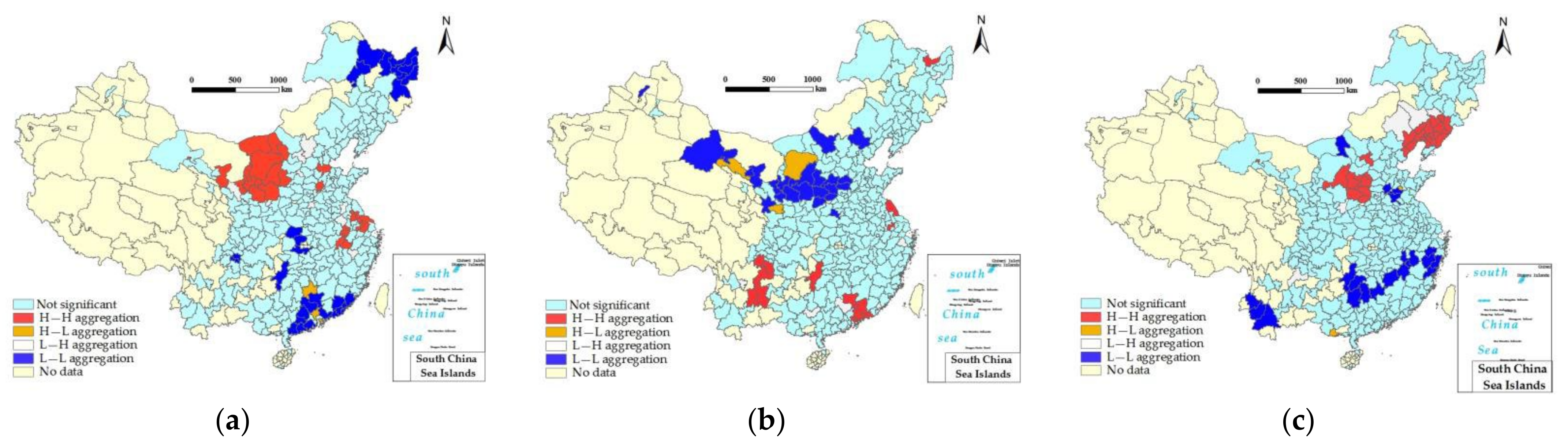
Figure 2.
The direction distribution of urban total factor carbon efficiency.

Figure 3.
Urban TFCE kernel density in the whole country (Nationwide) and the three regions (East; Central; West).
Figure 3.
Urban TFCE kernel density in the whole country (Nationwide) and the three regions (East; Central; West).

Table 1.
The Dagum Gini coefficients of total factor carbon efficiency in China and the three selected regions.
Table 1.
The Dagum Gini coefficients of total factor carbon efficiency in China and the three selected regions.
| Year | Gini Coefficient | Inner-Regional Difference | Inter-Regional Difference | Contribution Rate (%) | Inner-Regional Difference | Inter-Regional Difference | Hypervariable Density | ||||||
|---|---|---|---|---|---|---|---|---|---|---|---|---|---|
| East | Central | West | East-Central | EastWest | Central-West | Gw | Gnb | Gt | |||||
| 2005 | 0.1025 | 0.0886 | 0.1232 | 0.0888 | 0.1078 | 0.0908 | 0.1106 | 32.98 | 6.41 | 60.61 | 0.0338 | 0.0066 | 0.0621 |
| 2006 | 0.0624 | 0.0575 | 0.0896 | 0.0299 | 0.075 | 0.048 | 0.064 | 32.95 | 21.28 | 45.77 | 0.0206 | 0.0133 | 0.0286 |
| 2007 | 0.0489 | 0.0409 | 0.0563 | 0.0487 | 0.0492 | 0.0452 | 0.0529 | 33.29 | 8.57 | 58.14 | 0.0163 | 0.0042 | 0.0284 |
| 2008 | 0.0404 | 0.0308 | 0.0493 | 0.0405 | 0.0405 | 0.0362 | 0.0451 | 33.29 | 7.27 | 59.44 | 0.0135 | 0.0029 | 0.024 |
| 2009 | 0.047 | 0.0356 | 0.0556 | 0.0477 | 0.0468 | 0.0433 | 0.0525 | 32.91 | 12.5 | 54.6 | 0.0155 | 0.0059 | 0.0256 |
| 2010 | 0.0363 | 0.0338 | 0.0364 | 0.0377 | 0.0356 | 0.0368 | 0.0376 | 33.09 | 2.6 | 64.31 | 0.012 | 0.0009 | 0.0233 |
| 2011 | 0.0419 | 0.0362 | 0.0527 | 0.029 | 0.0452 | 0.0355 | 0.0462 | 32.61 | 20.27 | 47.12 | 0.0137 | 0.0085 | 0.0197 |
| 2012 | 0.0449 | 0.0343 | 0.0613 | 0.0351 | 0.0494 | 0.035 | 0.0499 | 33.39 | 20.17 | 46.44 | 0.015 | 0.0091 | 0.0209 |
| 2013 | 0.0444 | 0.0431 | 0.0354 | 0.0519 | 0.043 | 0.0487 | 0.045 | 32.17 | 3.27 | 64.56 | 0.0143 | 0.0015 | 0.0287 |
| 2014 | 0.0424 | 0.0387 | 0.0418 | 0.0453 | 0.0414 | 0.0424 | 0.0452 | 32.84 | 8.63 | 58.53 | 0.0139 | 0.0037 | 0.0248 |
| 2015 | 0.0367 | 0.0368 | 0.0284 | 0.0346 | 0.0343 | 0.0401 | 0.0414 | 30.38 | 14.56 | 55.06 | 0.0111 | 0.0053 | 0.0202 |
| 2016 | 0.0731 | 1003 | 0.0635 | 0.0413 | 0.0835 | 0.0784 | 0.0555 | 33.37 | 11.38 | 55.25 | 0.0244 | 0.0083 | 0.0404 |
| 2017 | 0.0799 | 0.0675 | 0.0856 | 0.0865 | 0.0774 | 0.0783 | 0.0863 | 33.17 | 3.39 | 63.44 | 0.0265 | 0.0027 | 0.0507 |
| 2018 | 0.0502 | 0.551 | 0.0507 | 0.0411 | 0.0538 | 0.0496 | 0.0471 | 33.3 | 2.3 | 64.4 | 0.0167 | 0.0012 | 0.0323 |
| 2019 | 0.0538 | 0.045 | 0.0621 | 0.0525 | 0.0547 | 0.0795 | 0.058 | 32.86 | 6.33 | 60.81 | 0.0177 | 0.0034 | 0.0327 |
| Mean | 0.0537 | 0.0496 | 0.0594 | 0.0474 | 0.0559 | 0.0505 | 0.0558 | 32.84 | 9.93 | 57.23 | 0.0177 | 0.0052 | 0.0308 |
Table 2.
The global Moran’s I index of spatial correlation.
| Year | I | E(I) | sd(I) | Z | P | Year | I | E(I) | sd(I) | Z | P |
|---|---|---|---|---|---|---|---|---|---|---|---|
| 2005 | 0.1973 | −0.0035 | 0.0005 | 9.3941 | 0.000 | 2013 | 0.0834 | −0.0035 | 0.0005 | 4.0757 | 0.001 |
| 2006 | 0.2094 | −0.0035 | 0.0005 | 9.9597 | 0.000 | 2014 | 0.1236 | −0.0035 | 0.0005 | 5.9676 | 0.000 |
| 2007 | 0.1094 | −0.0035 | 0.0005 | 5.2953 | 0.000 | 2015 | 0.0627 | −0.0035 | 0.0004 | 3.1753 | 0.000 |
| 2008 | 0.0506 | −0.0035 | 0.0005 | 2.5651 | 0.008 | 2016 | 0.1685 | −0.0035 | 0.0005 | 8.0759 | 0.000 |
| 2009 | 0.0273 | −0.0035 | 0.0002 | 2.0413 | 0.041 | 2017 | 0.0416 | −0.0035 | 0.0002 | 3.0631 | 0.002 |
| 2010 | 0.1068 | −0.0035 | 0.0005 | 5.2334 | 0.000 | 2018 | 0.1660 | −0.0035 | 0.0005 | 7.9190 | 0.000 |
| 2011 | 0.1055 | −0.0035 | 0.0004 | 5.2119 | 0.000 | 2019 | 0.2224 | −0.0035 | 0.0005 | 10.6588 | 0.000 |
| 2012 | 0.0925 | −0.0035 | 0.0004 | 4.6347 | 0.000 | - | - | - | - | - | - |
Table 3.
Standard deviational ellipse parameters.
| Year | Center (Longitude) | Center (Latitude) | Azimuth Angle | Minor Axis/Major Axis | Area (km2) |
|---|---|---|---|---|---|
| 2005 | 113.5349 | 33.1368 | 22.7495 | 0.7239 | 2,644,508.1170 |
| 2010 | 113.9322 | 33.0856 | 22.5042 | 0.6713 | 2,747,709.3789 |
| 2015 | 113.7475 | 32.8490 | 23.2948 | 0.6766 | 2,646,924.5017 |
| 2019 | 113.8674 | 33.0367 | 24.0191 | 0.6579 | 2,766,434.0552 |
Table 4.
The dynamic evolution characteristics of urban total factor carbon efficiency distributions.
Table 4.
The dynamic evolution characteristics of urban total factor carbon efficiency distributions.
| Region | Distribution Position | Distribution Main Peak Form | Distribution Ductility | Differentiation Trend |
|---|---|---|---|---|
| Overall | Moved left and right alternatively | The peak value first increased and then decreased and the width decreased | Right-trailing, convergent extension | Bipolar differentiation |
| AEast | Moved left and right alternatively | The peak value first increased and then decreased and the width decreased | Right-trailing, convergent extension | Multipolar differentiation |
| Central | Moved left and right alternatively | The peak value first increased and then decreased and the width first decreased and then increased | Right-trailing, convergent extension | Multipolar differentiation |
| West | Moved right | The peak increased and the width decreased | Right-trailing, convergent extension | Bipolar differentiation |
Table 5.
The traditional Markov transition probability matrix.
| t/t + 1 | Ⅰ | Ⅱ | Ⅲ | Ⅳ |
|---|---|---|---|---|
| Ⅰ | 0.4890 | 0.2190 | 0.1560 | 0.1360 |
| Ⅱ | 0.2400 | 0.3810 | 0.2790 | 0.1000 |
| Ⅲ | 0.0970 | 0.2880 | 0.3560 | 0.2590 |
| Ⅳ | 0.0450 | 0.1270 | 0.2650 | 0.5630 |
Table 6.
The spatial Markov transition probability matrix.
| Spatial Lag | t/t + 1 | Ⅰ | Ⅱ | Ⅲ | Ⅳ |
|---|---|---|---|---|---|
| Ⅰ | Ⅰ | 0.4490 | 0.1980 | 0.1700 | 0.1830 |
| Ⅱ | 0.2230 | 0.3500 | 0.3160 | 0.1120 | |
| Ⅲ | 0.0920 | 0.2860 | 0.3280 | 0.2940 | |
| Ⅳ | 0.1050 | 0.1740 | 0.2330 | 0.4880 | |
| Ⅱ | Ⅰ | 0.5860 | 0.2480 | 0.0950 | 0.0710 |
| Ⅱ | 0.2350 | 0.4050 | 0.2350 | 0.1250 | |
| Ⅲ | 0.0950 | 0.2770 | 0.3800 | 0.2480 | |
| Ⅳ | 0.0620 | 0.0970 | 0.2480 | 0.5930 | |
| Ⅲ | Ⅰ | 0.5270 | 0.2030 | 0.1830 | 0.1080 |
| Ⅱ | 0.2940 | 0.3500 | 0.2760 | 0.0800 | |
| Ⅲ | 0.1130 | 0.2580 | 0.3760 | 0.2540 | |
| Ⅳ | 0.0400 | 0.1340 | 0.2810 | 0.5450 | |
| Ⅳ | Ⅰ | 0.3580 | 0.2720 | 0.2220 | 0.1480 |
| Ⅱ | 0.2080 | 0.4310 | 0.2920 | 0.0690 | |
| Ⅲ | 0.0840 | 0.3270 | 0.3360 | 0.2520 | |
| Ⅳ | 0.0260 | 0.1180 | 0.2700 | 0.5860 |
Disclaimer/Publisher’s Note: The statements, opinions and data contained in all publications are solely those of the individual author(s) and contributor(s) and not of MDPI and/or the editor(s). MDPI and/or the editor(s) disclaim responsibility for any injury to people or property resulting from any ideas, methods, instructions or products referred to in the content. |
© 2022 by the authors. Licensee MDPI, Basel, Switzerland. This article is an open access article distributed under the terms and conditions of the Creative Commons Attribution (CC BY) license (https://creativecommons.org/licenses/by/4.0/).
Share and Cite
MDPI and ACS Style
Luo, H.; Qu, X. Spatiotemporal Evolution Trends of Urban Total Factor Carbon Efficiency under the Dual-Carbon Background. Land 2023, 12, 69. https://doi.org/10.3390/land12010069
AMA Style
Luo H, Qu X. Spatiotemporal Evolution Trends of Urban Total Factor Carbon Efficiency under the Dual-Carbon Background. Land. 2023; 12(1):69. https://doi.org/10.3390/land12010069
Chicago/Turabian StyleLuo, Haiyan, and Xiaoe Qu. 2023. "Spatiotemporal Evolution Trends of Urban Total Factor Carbon Efficiency under the Dual-Carbon Background" Land 12, no. 1: 69. https://doi.org/10.3390/land12010069
Note that from the first issue of 2016, this journal uses article numbers instead of page numbers. See further details here.