Article

Coupling Coordination between Park Green Space (PGS) and Socioeconomic Deprivation (SED) in High-Density City Based on Multi-Scale: From Environmental Justice Perspective

1
School of Architecture and Urban Planning, Shenzhen University, Shenzhen 518060, China
2
Shenzhen Key Laboratory for Optimizing Design of Built Environment, Shenzhen 518060, China
*
Author to whom correspondence should be addressed.
Land 2023, 12(1), 82; https://doi.org/10.3390/land12010082
Submission received: 26 November 2022 / Accepted: 23 December 2022 / Published: 27 December 2022
(This article belongs to the Section Urban Contexts and Urban-Rural Interactions)

Abstract

:
Several studies have revealed that park green space (PGS) plays a crucial role in improving residents’ quality of life and promoting sustainable development of the environment. However, rapid urbanization and population growth have led to an inequitable supply and demand for PGS, especially in high-density cities, which has been widely recognized as an important environmental justice issue. However, few studies have evaluated the equity and sustainability of PGS in high-density cities based on multi-scale. This study developed a framework to explore the spatial equity of PGS and its coupling coordination degree (CCD) with socioeconomic deprivation (SED) based on a multi-scale approach (pocket park, community park, and comprehensive park), then analyzed the spatial correlation between PGS and CCD. The results showed that: (1) The overall supply of 3-scale PGS does not meet residents’ demand for PGS resources in the study area and the urban center has the highest demand for PGS. (2) Among the three-scale PGS, the comprehensive PGS has the strongest supply capacity, but it also has the most severe supply–demand mismatch. (3) Although the service radius of pocket PGS is smaller than that of community PGS, the supply of pocket PGS is higher. (4) More than 95% of the studied area lacks coordination between PGS and SED development. (5) The subsystem that has the greatest spatial correlation with CCD in pocket PGS and comprehensive PGS was the number of configurations, while that in community PGS was the spatial arrangement. This study not only provides a theoretical reference for conducting research on PGS equity in high-density cities, but also provides a novel perspective on the sustainable, coordinated development and planning of urban PGS system.

1. Introduction

With the rapid development of urbanization around the world, the urban population density is increasing dramatically. By 2050, the world’s urban population will reach 2.5 billion, and 66% of the population is expected to live in cities [1]. Over the past few decades, the urbanization rate of developing Asian countries has increased significantly. Among them, China’s urbanization rate increased by 46.82% from 1978 to 2021, so it was awarded the title of “East Asian Miracle” [2]. Currently, scholars have defined “high-density city” in a variety of ways, but generally take urban population density as the main index. In this study, 15,000 residents/km² defined by Li is adopted as the standard of high-density city [3,4,5]. In the core urban agglomerations of China, high-density cities occupy more than half the urban space, which usually presents problems, such as social resources shortage, serious noise pollution, traffic congestion, and inequity in the distribution of ecological resources [6,7].
PGS is a kind of important ecological resource and green infrastructure which plays a vital role in improving human well-being and promoting sustainable urban development [8]. PGS not only provides a comfortable place for citizens to communicate, exercise, and relax, but also provides a variety of ecological environmental benefits to the city by regulating the microclimate [9], reducing noise [10], purifying the air [11], and so on. Meanwhile, studies have shown that during the global COVID-19 pandemic, PGS can relieve emotional stress [12] and enhance the resistance of residents [13], as well as reduce the risk of virus transmission [14].
Environmental justice was defined as “the principle that all residents and communities are entitled to equal protection of environmental and public health laws and regulations” [15]. It came from the civil rights movement in which the Americans underclass rallied against environmental pollution in the 1980s [16]. Scholars have divided its connotation into three dimensions: procedural justice, geographical justice, and social justice. Procedural justice mainly emphasizes the fairness and justice of environmental rights in the distribution system. Geographical justice pays more attention to the differences of environmental justice in geographical space. Social justice focuses on the fair distribution of environmental resources among different races and groups [17]. With the development of the environmental justice movement over the past two decades, scholars have been gradually concerned about the equity and justice of PGS [18]. The research on PGS equity can be divided into three stages: quantity equity, spatial equity, and social equity. In the era of urban incremental development, many researchers have used PGS quantity to measure PGS equity. In the stage of spatial equity, researchers paid more attention to the utilization efficiency and spatial allocation of PGS, and the “accessibility” and “per capita green space index” were used to quantify the PGS equity [19]. In the stage of social equity, the influence of economic and social factors on PGS equity was considered, and vulnerable groups became research objects [20,21]. The research topics included the discrepancies of PGS equity in different social groups or different areas with different economic levels [22,23].
In recent years, the issue of inequity supply and demand of PGS has become more and more serious in high-density cities [24], which has been recognized as an important environmental justice issue [25,26,27]. A few studies have evaluated the inequity of PGS supply from the perspective of urban needs, but there is lack of the evaluation of socioeconomic deprivation based on the characteristics of high-density cities [28,29]. Deprivation was first defined as a demonstrable disadvantage experienced by residents in wide society [30]. The socioeconomic deprivation of high-density cities can better represent the unmet needs of residents living in high-density cities. In terms of research scale, previous studies have usually explored the equity of the whole PGS [31,32]. However, PGS at different scales have different service capabilities [33], especially during the epidemic, when small-scale PGS, such as pocket parks and community parks, became the main outdoor activity places for citizens [34]. Therefore, it is necessary to study the equity of PGS at multiple scales.
The coupling coordination model is an important tool which can not only well reflect the close links and complex interactions between different systems, but also measure the sustainable development degree of areas [35,36]. At present, this model is mostly used to explore the sustainable coordination relationship between urban economy, society, and environment, e.g., the coupling coordination degree between population development and habitat quality [37], social economy and water resources [38,39], social economy and ecological environment [40,41], tourism development and ecological environment [42,43], society and resources, etc. [44]. Due to the typical supply–demand relationship between ecosystem services and social needs, some studies have focused on the coupling coordination between urban development and ecosystem service value, explaining the response of ecosystem service value to urbanization at different scales, such as country scale [45], urban agglomeration scale [46], and watershed scale [47], while very few studies have explored the coupling coordination degree of PGS equity and SED.
In summary, this study developed a framework to analyze the coupling coordination degree between PGS and SED in high-density city based on multi-scales from the perspective of environmental justice. The objectives of this study are: (1) Evaluate the PGS equity through three subsystems: quantity allocation, spatial arrangement, and accessibility. (2) Evaluate the SED in the high-density city through subsystems: population density, land use and building blocks. (3) Taking a grid as the research unit, calculate the supply–demand matching and coupling coordination degree of urban PGS and SED in three scales: pocket park, community park, and comprehensive park. (4) Analyze the spatial correlations between the subsystems of PGS and the coupling coordination degrees by using a geographically weighted regression model. (5) Put forward sustainable and coordinated development strategies for PGS of different scales. This study aims to provide a flexible operating framework that is applicable to other high-density cities for the study of PGS equity, and to provide a theoretical reference for the sustainable, coordinated development and planning of the urban PGS system.

2. Materials and Methods

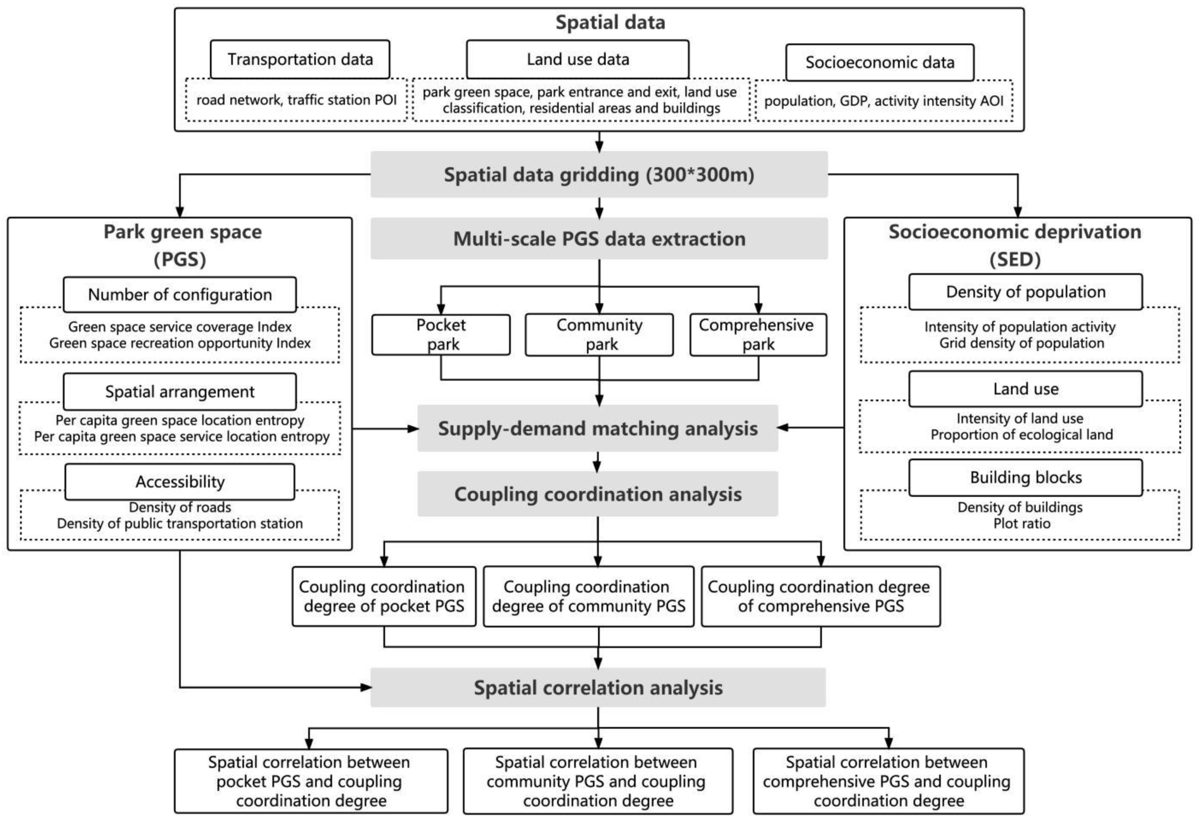
2.1. Study Framework

This study developed a multi-scale coupling coordination framework of PGS and SED to accurately explore PGS equity in high-density cities (Figure 1). The framework consists of three parts: (1) Divide PGS into three scales: pocket park, community park, and comprehensive park (Table 1). (2) Analyze the supply–demand matching and coupling coordination degree of PGS and SED. The PGS and SED both consist of three subsystems (Table 2). (3) Analyze the spatial correlation between PGS and CCD.

2.1.1. Study Scale and Study Unit of Analyses

The PGS were divided into three scales: comprehensive PGS, community PGS, and pocket PGS. PGS is frequently examined as a whole by researchers. However, PGS at various scales often have different service capacities (Table 1) [48]. At the same time, during the COVID-19 epidemic, many areas in China were governed by communities or even residential areas, and small-scale PGS, such as community PGS and pocket PGS, became the primary outdoor recreation spaces for residents [49]. In August 2022, the Ministry of Housing and Urban-Rural Development the residents’ Republic of China released a Notice on Promoting the Construction of “Pocket PGS”, focusing on accelerating small-scale PGS construction to provide more practical and accessible parks. Therefore, we divided the PGS into three scales and studied their spatial equity, respectively.
A 300 × 300 m grid serves as the study’s minimal research unit. Since 2013, the Chinese government began to implement grid management of metropolitan neighborhoods. However, previous studies merely took street or community as the minimum research unit. We hope to provide a more practical reference for grid management. Furthermore, the 300 × 300 m grid can reflect the difference in green space or population distribution in residential areas, so as to propose more refined management strategies.

2.1.2. Indexes Selection

(1) PGS
The PGS was evaluated in 3 aspects: number of configurations, spatial arrangement, and accessibility. First of all, PGS on different scales have different service radius. We used a network analysis method to calculate and visualize the service area of 3 PGS.
In terms of number of configurations, we chose green space service coverage (X1) and green space recreation opportunity (X2) indexes. When X1 is equal, the more PGS around the grid, the bigger X2 will be. Both indexes can measure the supply of PGS resources in the grid and reflect the regional equality of PGS.
In terms of number of spatial arrangements, we chose per capita green space location entropy (X3) and per capita green space service location entropy (X4) indexes. X3 reflects the level of PGS resources enjoyed by each person in the grid, and X4 reflects the level of effective PGS resources that residents in the grid can enjoy within a 15-min living circle. Both of them can reflect the spatial matching between green space and population, and reflect the spatial equity of PGS. In terms of number of accessibility, we chose density of roads (X5) and density of public transportation station (X6) indexes. X5 reflects the total length of roads leading to the PGS in the grid, and X6 reflects the number of stations leading to the park in the grid, both of which can represent the accessibility degree to the park.
(2) SED
In addition to the population density of more than 15,000 residents /km2, high-density cities also have obvious spatial features, including high land use intensity, scarce ecological resources, and high plot ratio. Therefore, we evaluated the SED of high-density cities in 3 aspects: density of population, land use and building blocks, including intensity of population activity (Y1), grid density of population (Y2), intensity of land use (Y3), proportion of ecological land (Y4), density of buildings (Y5), and plot ratio (Y6). Y4 is a negative index, because studies have shown that the lower the Y4, the higher the urbanization level and the demand for PGS resources [50], while the other five indexes are all positive indexes, which are positively correlated with the demand for PGS.

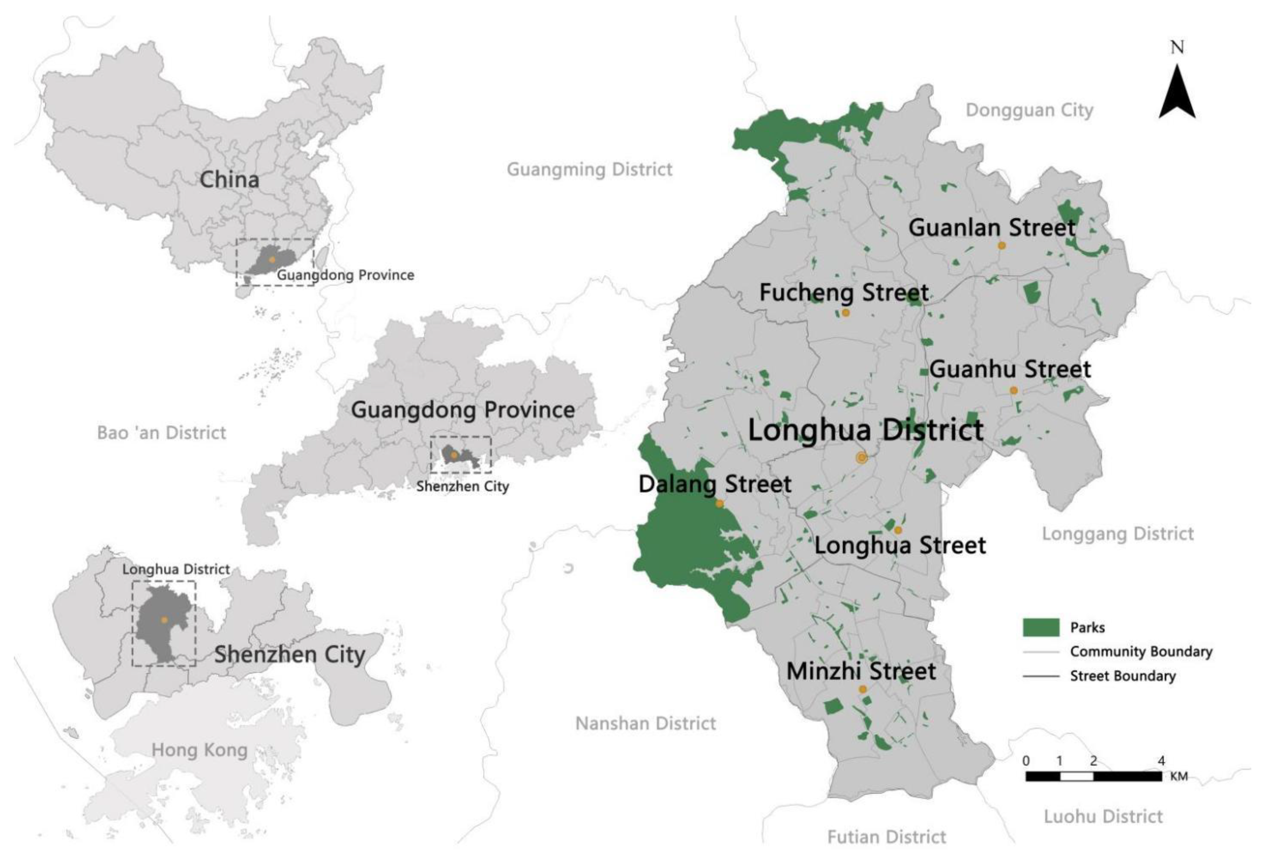
2.2. Study Area and Data

Longhua District is located on the urban development axis of Shenzhen, China, with a total area of 175.6 km2 (Figure 2). The area is one of the highly built-up areas and a typical high-density urban area in Shenzhen, with a population density of 15,957 residents/km2 in 2021. With the continuous growth of the urban population, the imbalance between supply and demand of PGS in Longhua District is more and more serious, so we selected it as the study area.
The park data came from the 2021 List of Shenzhen’s Parks and Green Spaces released by the Shenzhen Municipal Bureau of Urban Management and Comprehensive Law Enforcement. The traffic network data was downloaded from Open Street Map. The data of bus stations, park entrances, land use, residential areas, buildings, and activity points of interest (POI) were obtained from Baidu Map. The population and GDP data were downloaded from WorldPop website and the Resource and Environmental Science and Data Center of Chinese Academy of Sciences respectively, and supplemented by Shenzhen Statistical Yearbook and the Seventh National Population census for revision. All data are vectorized by ArcGIS and the projected coordinate system is WGS_84_UTM_Zone_49N. We chose the 300 m × 300 m grid as the study unit to explore the equity of PGS in high-density cities, so as to better guide the fine planning and management of urban PGS.

2.3. Methods

2.3.1. Entropy-Weighted Method

The entropy method can reflect the implied information from indexes objectively. From the statistical theory, the more discrete the selection index is, the smaller the entropy, and the larger the weight [51]. This method is widely used to solve multi-objective decision-making problems [52]. Here, the level of PGS and SED were evaluated by calculating the degree to which the target approached or deviated from the optimal and inferior solutions. The calculation steps are as follows:
Step one: Build the decision matrix.
H = ( h i j ) m × n , ( i = 1 , 2 , m ; j = 1 , 2 , n )
where j represents the criteria, and i denotes the observation.
Step two: Normalize the decision matrix.
r i j = h i j min ( h j ) max ( h j ) min ( h j ) , ( i = 1 , 2 , m ; j = 1 , 2 , n )
Step three: Calculate the information entropy.
e j = k i = 1 n p i j ln p i j , e j 0 , 1
p i j = r i j i = 1 m r i j , k = 1 ln m
Step four: Define the weight of the index j.
w j = 1 e j j = 1 n 1 e j
Step five: Calculate the composite index j.
Z j = j = 1 n r j × w j

2.3.2. Supply-Demand Matching Model

In order to analyze the quantitative matching characteristics of PGS and SED, the PGS and SED were standardized by Z-Score. The x-axis represents the standardized PGS and the y-axis represents the standardized SED. Then, the standardized results are divided into quadrants. 0 is taken as the critical value of the data standardization, which can observe and compare the matching types of supply–demand and their changes more concisely. It has been widely used in the spatial differentiation and imbalance of supply–demand [53,54,55]. The research area is divided into two types of supply–demand matching: supply–demand mismatching (including PGS supply advanced, PGS supply lagged), and supply–demand matching (including Low balanced and High balanced) (Table 3). The calculation steps are as follows:
x = x i x s
x = 1 n i = 1 n x i
s = 1 n i = 1 n ( x x ) 2
where x is standardized PGS or SED, xi is the PGS or SED value of the ith grid, x is the average value of the region, s is the standard deviation of the area, and n is the total number of grid units.

2.3.3. Coupling Coordination Model

Coupling coordination, a concept from physics, refers to the interaction and influence within a system or between the system elements. Coupling coordination degree models (CCDM) have been widely used in the nature, economic, and societal fields, which can explain the sustainability of the whole system [56]. We established the coupling coordination model of PGS and SED and the calculation steps were presented as follows:
C = 2 u 1 u 2 u 1 + u 2 2
T = a u 1 + b u 2
C C D = T × U
where u1 and u2 represent the total quantity of PGS and SED, respectively. T represents the coupling degree and CCD represents the coupling coordination degree between the two systems. a and b represent the weights of the two systems and are used to measure the importance of each system (a + b = 1). Since the PGS system is as important as the SED system, the weight of each subsystem is by default equal, i.e., a = b = 0.5. According to pertinent studies [57,58], CCD was divided into 3 classes (Table 4): coordinated class indicates that the development of PGS and SED is not coordinated and the sustainability is weak. Transitional class indicates moderately coordinated and sustainable development between PGS and SED. Coordinated class indicates highly coordinated and sustainable development between PGS and SED.

2.3.4. Geographically Weighted Regression (GWR)

Geographically weighted regression (GWR) is a geo-statistical method that incorporates spatial characteristics into the model in the way of distance weighting on the basis of the traditional least square model and allows local parameter estimation [59]. Spatial data are usually characterized by spatially non-stationarity, and the analysis results of fitting spatial data with a general linear regression model cannot completely reflect the real characteristics of spatial data, while the GWR can effectively detect spatially non-stationarity and allow different spatial relationships in different geographic spaces [56]. Therefore, GWR can be used to establish a local regression equation at each grid point within the spatial range to explore the spatial heterogeneity of factors affecting the coupling coordination degree of different types of parks at the grid scale. The calculation formula is as follows:
y i = β 0 ( u i , v i ) + j = 1 k β j ( u i , v i ) χ i j + ε i
In this study, yi is the coupling coordination degree of the ith grid, (ui, vi) is the spatial geographic coordinate of the ith grid, is the fixed-effect intercept of (ui, vi), Xij is the value of the green land resource equity evaluation index j of the ith grid (j = 1,2..., k), βj is the regression coefficient of Xij, εi is the random error. In this paper, AICc with stronger compatibility was used to determine the bandwidth for GWR analysis. R2 and adjusted R2 were used to compare the fit of OLS and GWR models. The smaller the AICc value, the closer R2 and adjusted R2 were to 1, the better the model fit.

3. Results

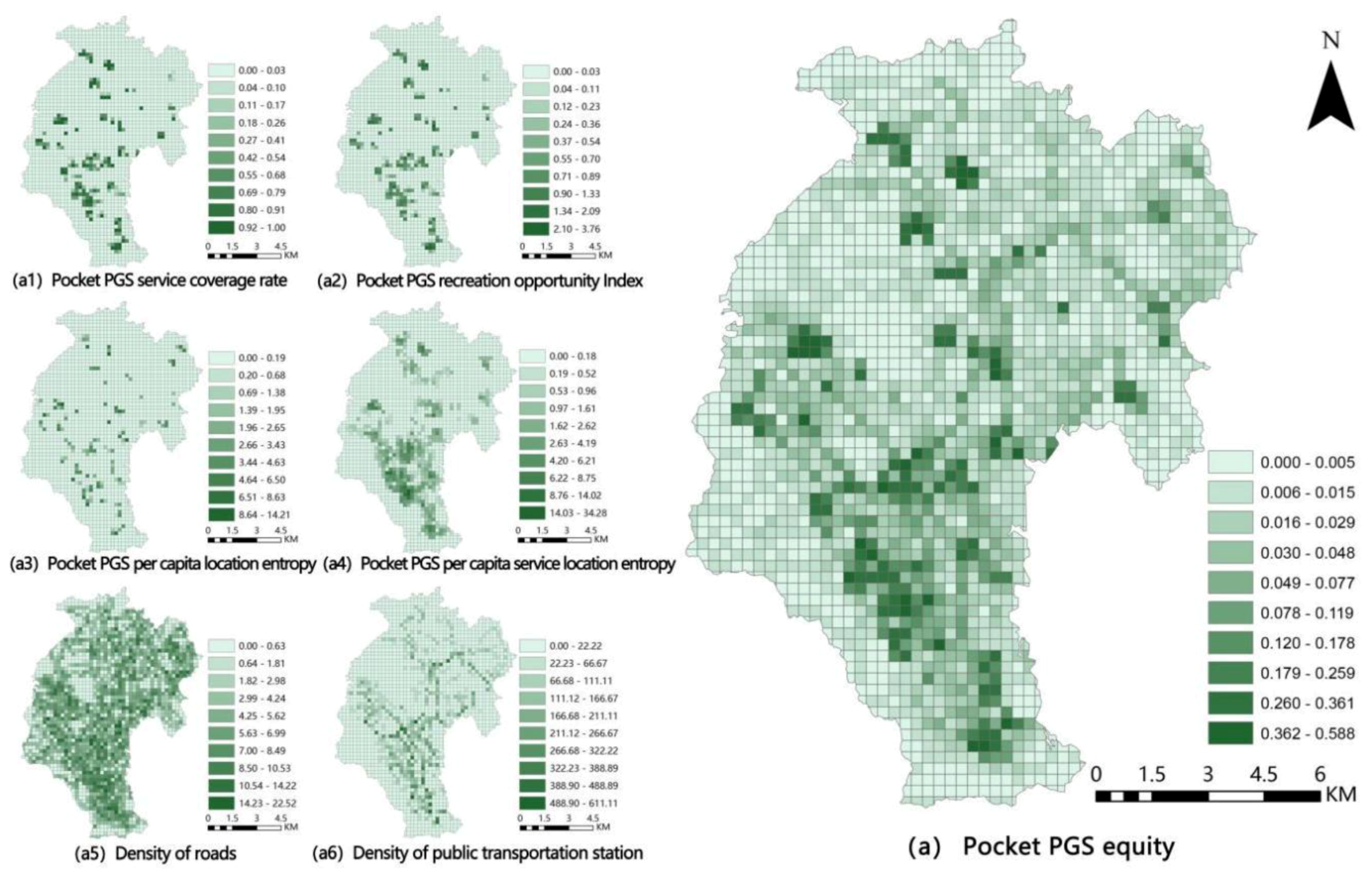
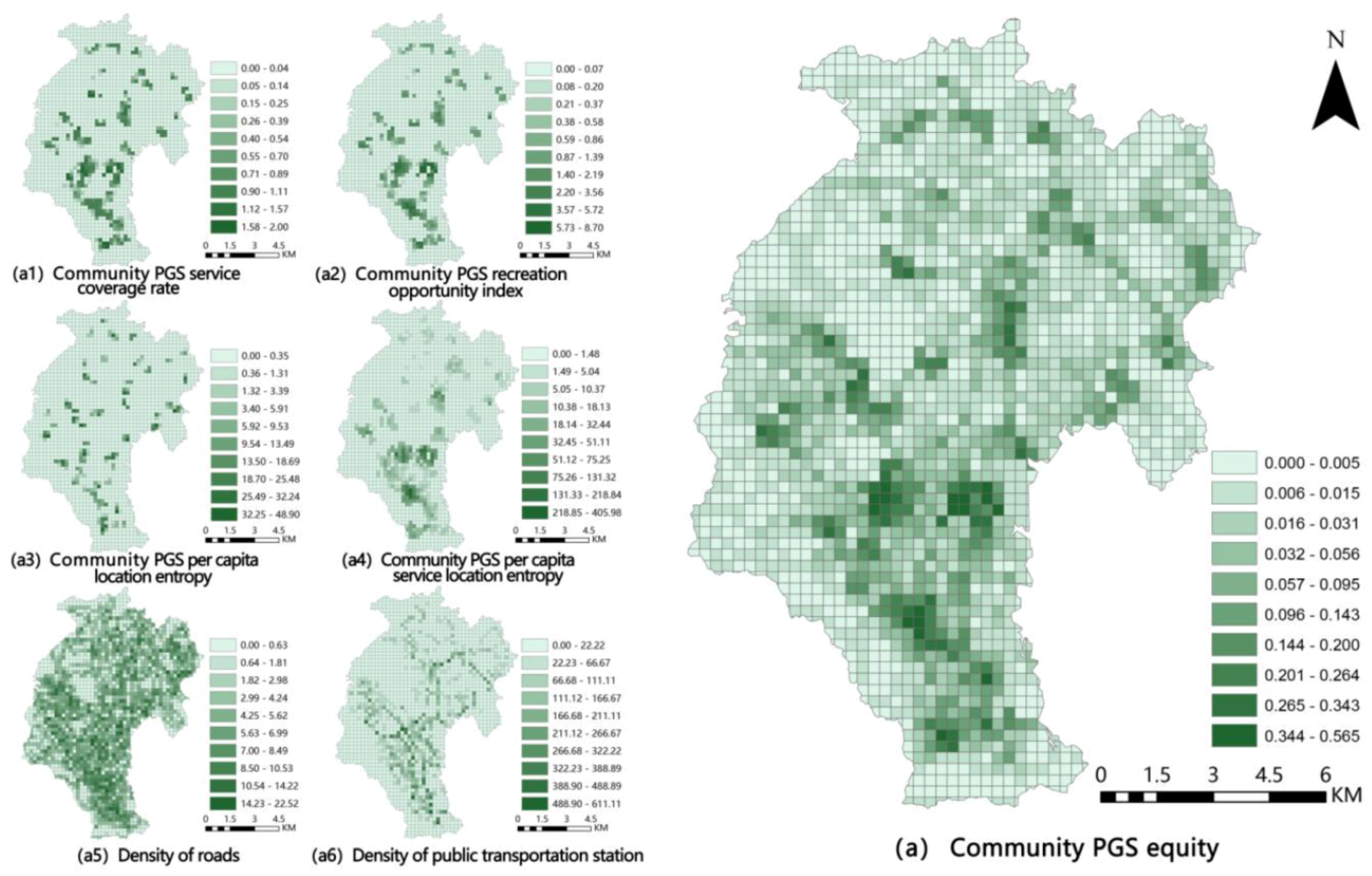
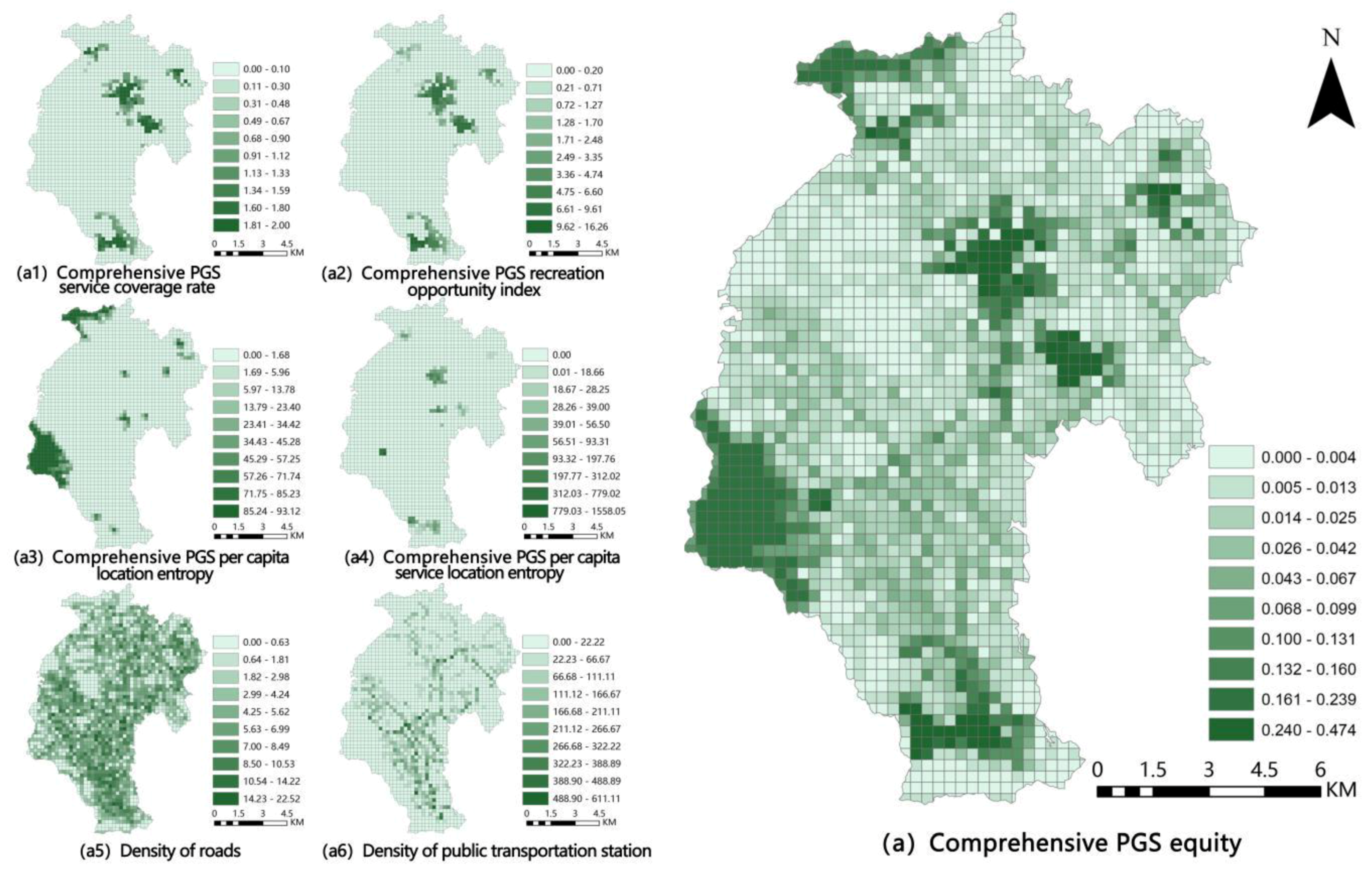
3.1. Multi-Scale Park Green Space (PGS) Equity

The entropy method was used to calculate the weights of subsystems and indexes, and the supply quantities of three-scale PGS were calculated and visualized (Table 5, Figure 3, Figure 4 and Figure 5). It can be seen that comprehensive PGS has the strongest supply capacity, followed by pocket PGS and community PGS. The strong supply capacity area of comprehensive PGS is obviously concentrated in six locations, but these locations are relatively independent, so there is no comprehensive PGS supply in the urban center, resulting in the spatial inequity (Figure 5a). Compared with community PGS, pocket PGS has a smaller service radius, but because it is located nearer to residential areas, more residents enjoy its services, increasing its overall supply over that of community PGS. From the perspective of spatial pattern, the locations with a high supply of pocket PGS and community PGS are more concentrated in the southern urban center, resulting in an unequal supply of PGS in the northern and peripheral areas (Figure 3a and Figure 4a).

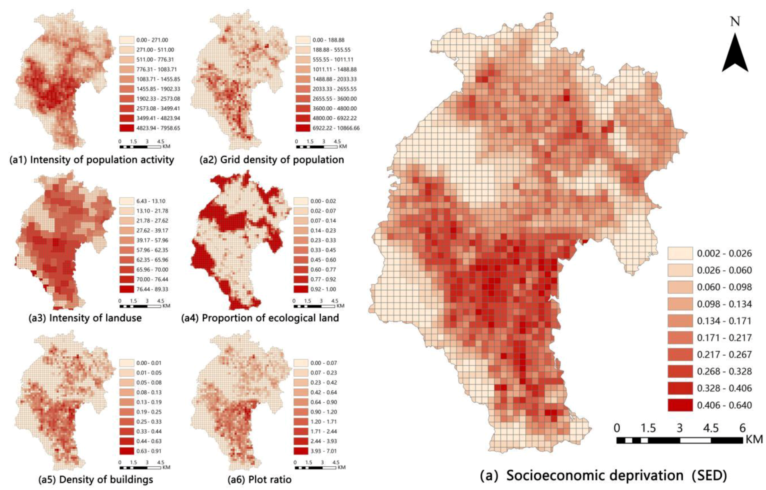
3.2. High-Density Urban Socioeconomic Deprivation (SED)

The entropy method was used to calculate the weights of the three subsystems of SED, and the demand quantities of SED were calculated and visualized (Table 6, Figure 6). First of all, the total demand of SED (295.57) is higher than the sum of three-scale PGS supply, indicating that the overall PGS supply in the study area does not meet residents’ demand for PGS resources. From the perspective of spatial pattern, the high demand SED areas mainly concentrated in the southern urban center, with a decreasing trend from the center to the periphery. This is due to the high density of residents, traffic, and commerce in the urban center, resulting in the high demand for PGS there. Compared with the southern area, the northern area has a sparse population, relatively late development, and construction, resulting in low demand for PGS. There are several obvious low-SED areas in the study area, which are large ecological lands, such as mountains, forest parks, and reservoirs. They are rich in green space resources themselves, so the demand for green space resources is very low.

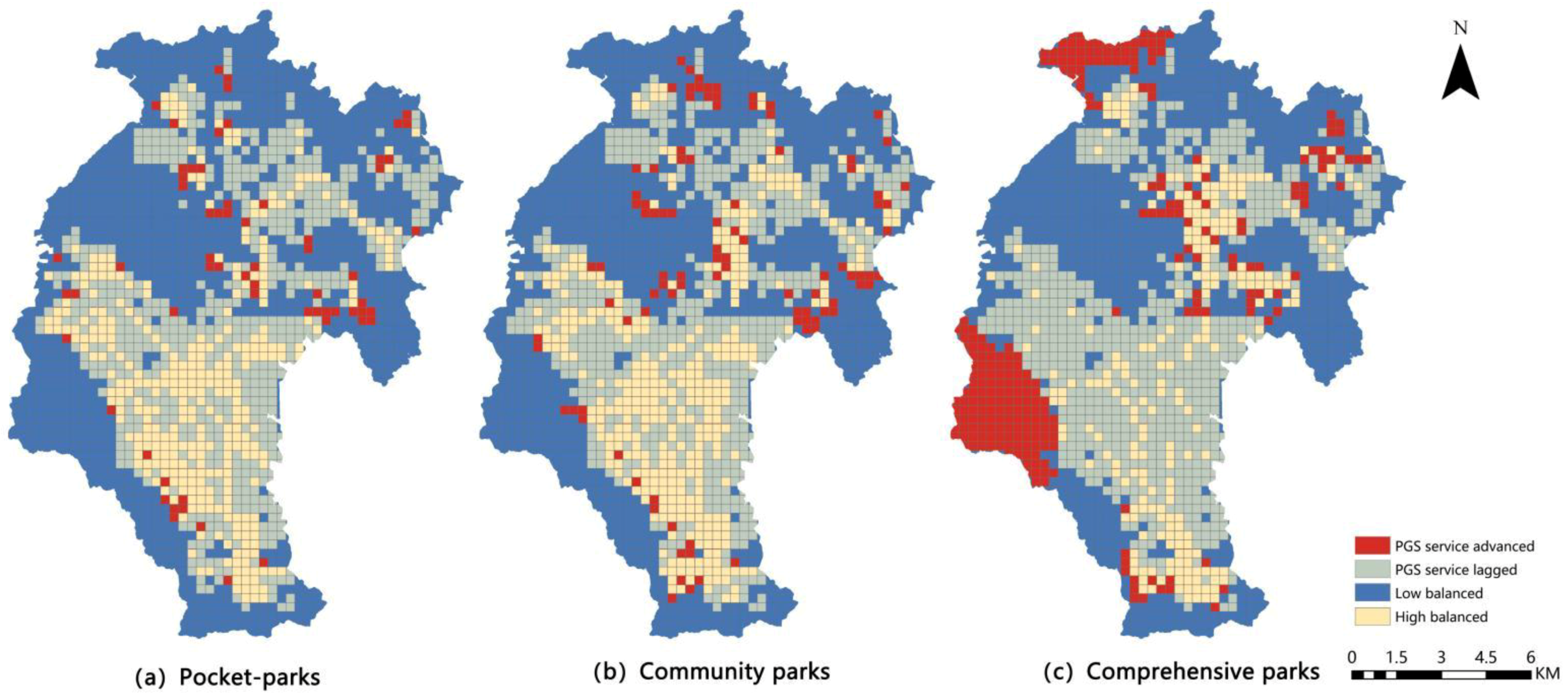
3.3. PGS-SED Supply-Demand Matching

The relationship between PGS and SED was calculated through the supply–demand matching method (Table 7, Figure 7). It can be seen that the most serious supply–demand mismatching is comprehensive PGS, among which 31.75% of the areas are PGS supply lagged areas, that is, residents’ demand for comprehensive PGS in these areas is unsatisfactory. Pockets and community PGS are similar in the proportion of areas where supply and demand mismatches, but there are more areas where pocket PGS supply lags than community parks. According to Section 3.1, the total PGS supply comprises comprehensive PGS, pocket PGS, and community PGS in order from most to least. However, after matching with SED, the PGS supply lagged area is in the opposite order, indicating that the spatial arrangement of comprehensive PGS and pocket PGS exacerbates the spatial inequity of PGS. Although the comprehensive PGS has the strongest service capacity, the service scope does not cover the urban center, which results in a large number of residents being unable to conveniently enjoy the services of the comprehensive park. For pocket PGS and community PGS, about a half of the urban center remains classified as a PGS supply lagged area, as residents in these areas do not have equal access to each scale of PGS.

3.4. PGS-SED Coupling Coordination

After the supply–demand matching analysis between PGS and SED, the coupling coordination model is adopted to analyze the coupling coordination degree (CCD) between PGS and SED (Table 8, Figure 8), so as to better propose strategies to promote the spatial equity and sustainable development of PGS. It is clear that, regardless of PGS type, more than 95% of the study area is uncoordinated between PGS and SED, and the comprehensive PGS even has no coordination area. In terms of spatial pattern, the high CCD area of pocket and community PGS cluster in the southern urban center and the transition class and coordinated class of the comprehensive PGS have two obvious clusters in the urban center and southernmost areas, which are also the areas with high balanced matching level between PGS and SED.

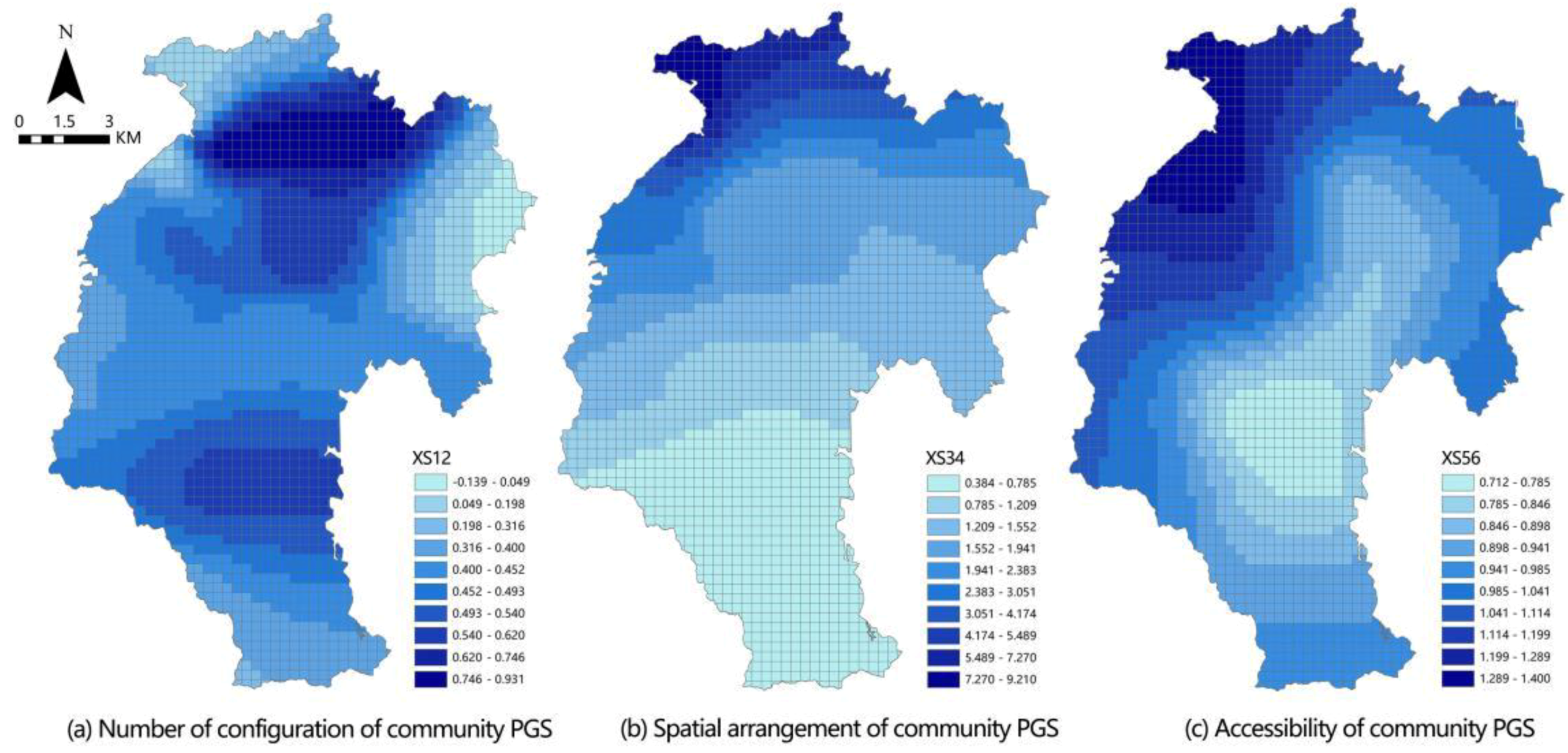
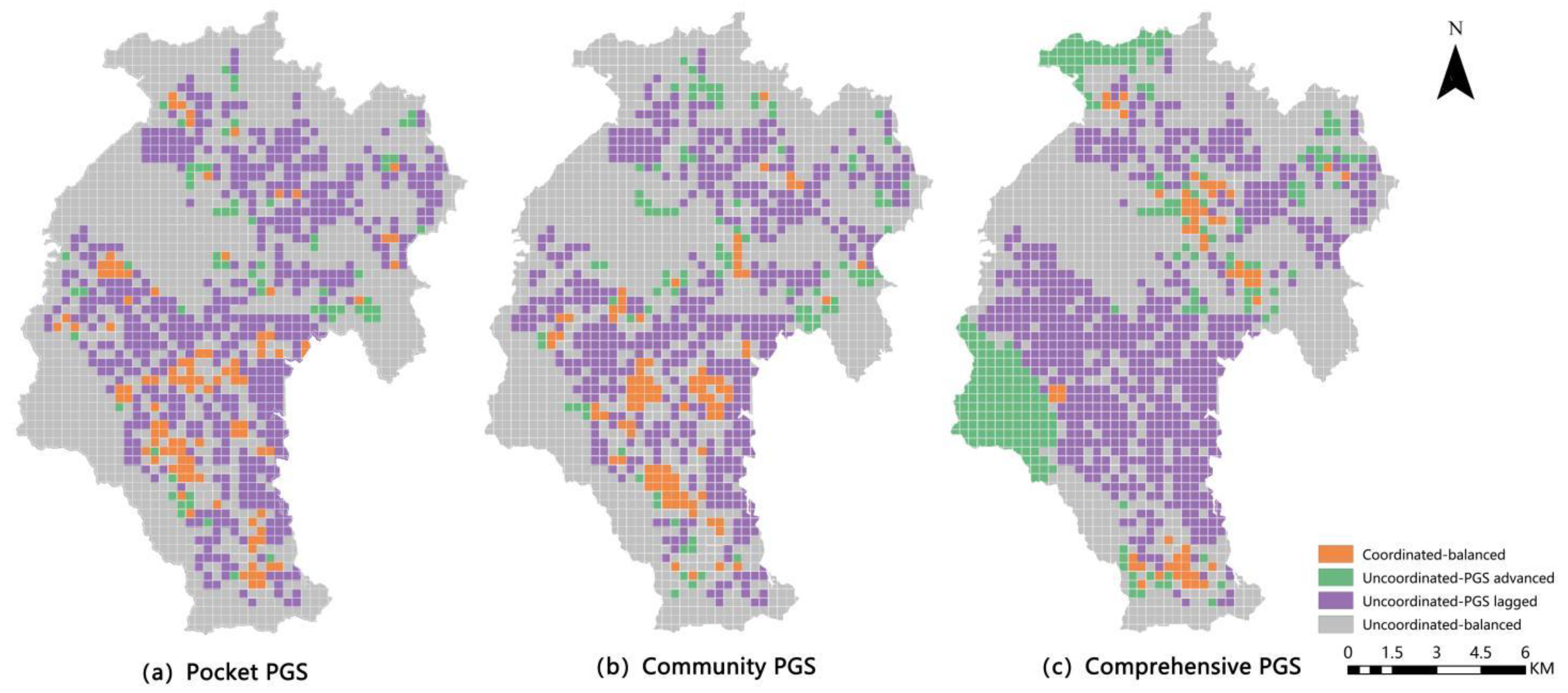
3.5. Spatial Correlation between PGS and Coupling Coordination Degree

The indexes system was constructed to analyze the spatial correlation between three scales of PGS and coupling coordination degree (CCD). In this model, three CCD were taken as dependent variables. Six indexes of the PGS were taken as independent variables (Table 9). As can be seen from Table 10, for pocket PGS, the number of configurations is the subsystem that affects the coupling coordination degree (CCD) most (Figure 9). It is clear that residents in south area enjoy more pocket PGS than the north, and the number of pocket PGS and the distance from residential areas are key factors affecting the spatial equity of pocket PGS. The CCD of community PGS is similar to that of pocket PGS, but the biggest factor affecting community PGS is spatial arrangement, which indicates that in the northern area, community PGS should be arranged more within the 15-min living circle of the residential area, and more entrances and exits should be provided, so that residents can enjoy community PGS resources more conveniently (Figure 10). For comprehensive PGS, the southern area with high CCD is mainly affected by the number of configurations and spatial arrangement subsystems. The low CCD in the northern periphery is caused by the accessibility subsystem. Therefore, for comprehensive PGS, it is necessary to strengthen the connection between the northern periphery and the central area, as well as increase bus routes and bus stations, so as to enable a wider range of residents to enjoy comprehensive PGS conveniently and thereby increase spatial equity (Figure 11).

4. Discussion

4.1. Multi-Scale Coupling Coordination Model and Indexes Selection

This study analyzed the spatial coupling coordination between PGS and SED. In terms of the indexes of PGS equity, most of the previous studies chose the quantity and quality indexes, while the spatial arrangement and accessibility of PGS were less evaluated for PGS equity [60,61,62,63]. In this study, three subsystems, i.e., number of configurations, spatial arrangement, and accessibility, were selected for a total of six indexes, which can relatively comprehensively evaluate PGS equity. In terms of SED, previous studies used indexes such as the proportion of residents of different ages and income to evaluate it, but there was a lack of SED evaluation for high-density cities [28]. High-density cities have obvious characteristics in population density and space environment, so this study put forward the evaluation indexes of SED in high-density cities, including six indexes in three subsystems: population density, land use, and building blocks, which were more targeted. PGS on different scales often have different service capabilities. This study divided PGS into three scales: pocket park, community park, and comprehensive park. At the same time, the spatial pattern of the PGS equity and coupling coordination could be seen clearly using grid visualization, which is conducive to putting forward fine management and development strategies.

4.2. Development Proposals for Spatial Equity of 3-Scale PGS

We analyzed the supply–demand matching and coupling coordination degree (CCD) between PGS and SED and studied the influencing factors affecting the CCD. Based on these, the study area was divided into four parts: uncoordinated-PGS advanced area, uncoordinated-PGS lagged area, uncoordinated-balanced area, coordinated-balanced area (Figure 12).
Uncoordinated-PGS advanced area indicates that the supply of PGS exceeds the total demand of PGS required by residents, but the development of the PGS and SED is not coordinated, and if not controlled, the spatial inequity of PGS will be exacerbated over time. It can be seen that there are two obvious uncoordinated-PGS advanced areas of comprehensive PGS (Figure 12c). This is because there is a large area of natural PGS in the area, and the service radius of these PGS can be improved by increasing the entrances, roads, and bus stations available to parks, so that more residents can enjoy their services conveniently.
Uncoordinated-PGS lagged area indicates that PGS there cannot meet residents’ demand of PGS, and the development between PGS and SED is not coordinated. The uncoordinated-PGS lagged areas of the three-scale PGS all cluster in the southern area, and the comprehensive PGS is more obvious. This area is a high-density urban center with a large population, dense residential areas and roads. Therefore, combined with the urban micro-renewal policy, we can vigorously promote the construction of pocket PGS along the road, gradually build the PGS avenues, and adjust the location of the community PGS to ensure that residents can cover the entrance to the community PGS within 15 min living circle, achieving full service coverage for the PGS in high-density areas.
Uncoordinated-balanced area indicates that PGS is able to meet residents’ demand for PGS there, but the PGS supply cannot keep up with the SED increase, and the supply tends to lag behind, which will exacerbate the spatial inequity of PGS. The uncoordinated-balanced areas are mainly in the periphery, with a good ecological base and a large area of reservoirs, mountains, golf courses, etc., which can be developed into country PGS, with a well-developed green-road system to extend its service radius to the high-density urban center.

4.3. Limitations of the Study and Future Plans

Firstly, compared with the street or community unit, using grid as the minimum study unit to analyze the PGS configuration is better to refine the spatial analysis and guide the planning and development, but the use of grid requires higher resolution of data. For example, 300 m × 300 m grid was used in this study, while the smallest resolution of GDP raster data that could be found was 1 km*1 km, resulting in equal values of multiple adjacent grids, which cannot distinguish spatial differences clearly. At the same time, different resolution of the grid will affect the accuracy of the results. According to the actual scale of residential areas and referring to previous studies, this study determined a grid of 300*300 [64], lacking discussion on grids of other resolutions.
Secondly, this study used the density of road and the density of bus stations to represent the accessibility, for they’re more conducive to reflect the spatial differences in the grids. However, at present, there are many methods to calculate accessibility, such as the buffer method, network analysis method, two-step floating catchment area method, and mobile phone signaling data method [65,66,67,68]. In the future, we plan to further explore the differences in accessibility and spatiotemporal evolution of different types of PGS.
Finally, the framework which was developed in this study needs further refinement. In the next step, we plan to quantify users’ evaluation of PGS through questionnaire surveys and incorporate the quality of PGS into the research framework to improve the accuracy of the research.

5. Conclusions

From the perspective of environmental justice, this study analyzed the equity of PGS of three scales and explored the supply–demand matching and coupling coordination degree (CCD) between PGS and SED in a high-density city. Then, the spatial correlation between PGS and CCD was analyzed, and sustainable development strategies were proposed for three PGSs. The study presents the following conclusions:
(1) The demand for three-scale PGS resources is higher than the overall supply in the study area.
(2) PGS resources are most in demand in high-density city center, where they are also frequently confined and become PGS supply lagged area.
(3) The comprehensive PGS has the best supply capacity among three-scale PGS, but it also has the most severe supply–demand mismatch. Because its service area is far away from the urban center, residents there cannot enjoy the services of comprehensive PGS conveniently.
(4) Although the service radius of pocket PGS is smaller than community PGS, it has a higher supply because it is located adjacent to residential areas, which increases the recreation opportunity in pocket PGS for residents.
(5) The development between PGS and SED is not coordinated in more than 95% of the study area, and most of the uncoordinated area at the periphery is of low balanced supply–demand matching type. Without proper planning, the supply of PGS will not meet residents’ demand in the area.
(6) For pocket PGS, the number of configurations is the subsystem that affects the CCD most. However, the most important factor affecting community PGS is spatial arrangement. For comprehensive PGS, the number of configurations and spatial arrangement are the subsystems that affect the CCD most, while that in the northern periphery is caused by the accessibility subsystem.

Author Contributions

Conceptualization, S.H. and C.W.; methodology, S.H.; software, S.H., M.D. and Y.C.; validation, S.H., M.D. and Y.C.; formal analysis, S.H.; investigation, S.H. and C.W.; resources, S.H. and C.W.; data curation, S.H.; writing—original draft preparation, S.H., M.D. and Y.C.; writing—review and editing, S.H. and C.W.; visualization, S.H.; supervision, S.H. and C.W.; project administration, S.H. and C.W. All authors have read and agreed to the published version of the manuscript.

Funding

This research received no external funding.

Data Availability Statement

The data presented in this study are available on request from the corresponding author.

Acknowledgments

We would like to thank the Urban Management Bureau and the Comprehensive Law Enforcement Bureau of Shenzhen Municipality for providing the park data in the study area.

Conflicts of Interest

The authors declare that they have no conflict of interest.

References

  1. UN-DESA. World Urbanization Prospects; Department of International Economic and Social Affairs: New York, NY, USA, 2018. [Google Scholar]
  2. Zhang, X.; Wan, G.; Luo, Z.; Wang, C. Explaining the East Asia miracle: The role of urbanization. Econ. Syst. 2019, 43, 100697. [Google Scholar] [CrossRef]
  3. Ming, C.; Fan, J. Carbon reduction in a high-density city: A case study of Langham Place Hotel Mongkok Hong Kong. Renew. Energy 2013, 50, 433–440. [Google Scholar]
  4. Wang, D.; Wang, P.; Chen, G.; Liu, Y. Ecological-social-economic system health diagnosis and sustainable design of high-density cities: An urban agglomeration perspective. Sustain. Cities Soc. 2022, 87, 104177. [Google Scholar] [CrossRef]
  5. Li Min, Y.C. Threshold standard and global distribution of high-density cities. World Reg. Stud. 2015, 1, 38–45. [Google Scholar]
  6. Mouratidis, K. Compact city, urban sprawl, and subjective well-being. Cities 2019, 92, 261–272. [Google Scholar] [CrossRef]
  7. Tian, Y.H.; Jim, C.Y.; Tao, Y. Challenges and Strategies for Greening the Compact City of Hong Kong. J. Urban Plan. Dev. 2012, 138, 101–109. [Google Scholar] [CrossRef]
  8. Liu, B.; Tian, Y.; Guo, M.; Tran, D.; Alwah, A.A.Q.; Xu, D. Evaluating the disparity between supply and demand of park green space using a multi-dimensional spatial equity evaluation framework. Cities 2022, 121, 103484. [Google Scholar] [CrossRef]
  9. Das, M.; Das, A.; Momin, S. Quantifying the cooling effect of urban green space: A case from urban parks in a tropical mega metropolitan area (India). Sustain. Cities Soc. 2022, 87, 104062. [Google Scholar] [CrossRef]
  10. Schäffer, B.; Brink, M.; Schlatter, F.; Vienneau, D.; Wunderli, J.M. Residential green is associated with reduced annoyance to road traffic and railway noise but increased annoyance to aircraft noise exposure. Environ. Int. 2020, 143, 105885. [Google Scholar] [CrossRef]
  11. Yao, Y.; Wang, Y.; Ni, Z.; Chen, S.; Xia, B. Improving air quality in Guangzhou with urban green infrastructure planning: An i-Tree Eco model study. J. Clean. Prod. 2022, 369, 133372. [Google Scholar] [CrossRef]
  12. Pouso, S.; Borja, Á.; Fleming, L.E.; Gómez-Baggethun, E.; White, M.P.; Uyarra, M.C. Contact with blue-green spaces during the COVID-19 pandemic lockdown beneficial for mental health. Sci. Total Environ. 2021, 756, 143984. [Google Scholar] [CrossRef] [PubMed]
  13. Yang, Y.; Lu, Y.; Jiang, B. Population-weighted exposure to green spaces tied to lower COVID-19 mortality rates: A nationwide dose-response study in the USA. Sci. Total Environ. 2022, 851, 158333. [Google Scholar] [CrossRef] [PubMed]
  14. Bustamante, G.; Guzman, V.; Kobayashi, L.C.; Finlay, J. Mental health and well-being in times of COVID-19: A mixed-methods study of the role of neighborhood parks, outdoor spaces, and nature among US older adults. Health Place 2022, 76, 102813. [Google Scholar] [CrossRef] [PubMed]
  15. Wade, R. Dumping in Dixie: Race, Class and Environmental Quality.by Robert D. Bullard. Contemp. Sociol. 1991, 20, 911–912. [Google Scholar] [CrossRef]
  16. Burke, L.M. Race and Environmental Equity: A Geographic Analysis in Los Angeles. Geogr. Inf. Syst. 1993, 3, 44–50. [Google Scholar]
  17. Bullard, R. Dumping in Dixie: Race, Class, and Environmental Quality; Westview Press: Boulder, US, 2000. [Google Scholar]
  18. Alessandro Rigolon, M.F.B.H. An Ecological Model of Environmental Justice for Recreation. Leis. Serv. 2022, 44, 655–676. [Google Scholar] [CrossRef]
  19. Guo, S.; Song, C.; Pei, T.; Liu, Y.; Ma, T.; Du, Y.; Chen, J.; Fan, Z.; Tang, X.; Peng, Y.; et al. Accessibility to urban parks for elderly residents: Perspectives from mobile phone data. Landsc. Urban Plan. 2019, 191, 103642. [Google Scholar] [CrossRef]
  20. Fe, A.; Nka, B. Urban green spaces for the social interaction, health and well-being of older people—An integrated view of urban ecosystem services and socio-environmental justice—ScienceDirect. Environ. Sci. Policy 2020, 109, 36–44. [Google Scholar]
  21. Zhang, J.; Yu, Z.; Cheng, Y.; Chen, C.; Wan, Y.; Zhao, B.; Vejre, H. Evaluating the disparities in urban green space provision in communities with diverse built environments: The case of a rapidly urbanizing Chinese city. Build. Environ. 2020, 183, 107170. [Google Scholar] [CrossRef]
  22. Hoffimann, E.; Barros, H.; Ribeiro, A. Socioeconomic Inequalities in Green Space Quality and Accessibility—Evidence from a Southern European City. Int. J. Environ. Res. Public Health 2017, 14, 916. [Google Scholar] [CrossRef] [Green Version]
  23. Wu, L.; Kim, S.K.; Lin, C. Socioeconomic groups and their green spaces availability in urban areas of China: A distributional justice perspective. Environ. Sci. Policy 2022, 131, 26–35. [Google Scholar] [CrossRef]
  24. Shadman, S.; Ahanaf Khalid, P.; Hanafiah, M.M.; Koyande, A.K.; Islam, M.A.; Bhuiyan, S.A.; Sin Woon, K.; Show, P. The carbon sequestration potential of urban public parks of densely populated cities to improve environmental sustainability. Sustain. Energy Technol. Assess. 2022, 52, 102064. [Google Scholar] [CrossRef]
  25. Du, S.; He, H.; Liu, Y.; Xing, L. Identifying Key Factors Associated with Green Justice in Accessibility: A Gradient Boosting Decision Tree Analysis. Int. J. Environ. Res. Public Health 2022, 19, 10357. [Google Scholar] [CrossRef] [PubMed]
  26. Dai, D. Racial/ethnic and socioeconomic disparities in urban green space accessibility: Where to intervene? Landsc. Urban Plan. 2011, 102, 234–244. [Google Scholar] [CrossRef]
  27. Wolch, J.R.; Byrne, J.; Newell, J.P. Urban green space, public health, and environmental justice: The challenge of making cities ‘just green enough’. Landsc. Urban Plan. 2014, 125, 234–244. [Google Scholar] [CrossRef] [Green Version]
  28. Zhang, R.; Zhang, C.-Q.; Cheng, W.; Lai, P.C.; Schüz, B. The neighborhood socioeconomic inequalities in urban parks in a High-density City: An environmental justice perspective. Landsc. Urban Plan. 2021, 211, 104099. [Google Scholar] [CrossRef]
  29. You, H. Characterizing the inequalities in urban public green space provision in Shenzhen, China. Habitat Int. 2016, 56, 176–180. [Google Scholar] [CrossRef]
  30. Townsend, P.; Phillimore, P.; Beattie, A. Health and Deprivation: Inequality and the North; Croom Helm: Wolfeboro, London, 1988. [Google Scholar]
  31. Yang, G.; Zhao, Y.; Xing, H.; Fu, Y.; Liu, G.; Kang, X.; Mai, X. Understanding the changes in spatial fairness of urban greenery using time-series remote sensing images: A case study of Guangdong-Hong Kong-Macao Greater Bay. Sci. Total Environ. 2020, 715, 136763. [Google Scholar] [CrossRef]
  32. Li, X.; Huang, Y.; Ma, X. Evaluation of the accessible urban public green space at the community-scale with the consideration of temporal accessibility and quality. Ecol. Indic. 2021, 131, 108231. [Google Scholar] [CrossRef]
  33. Zheng, Z.; Shen, W.; Li, Y.; Qin, Y.; Wang, L. Spatial equity of park green space using KD2SFCA and web map API: A case study of zhengzhou, China. Appl. Geogr. 2020, 123, 102310. [Google Scholar] [CrossRef]
  34. Zhang, S.; Yu, P.; Chen, Y.; Jing, Y.; Zeng, F. Accessibility of Park Green Space in Wuhan, China: Implications for Spatial Equity in the Post-COVID-19 Era. Int. J. Environ. Res. Public Health 2022, 19, 5440. [Google Scholar] [CrossRef] [PubMed]
  35. Kong, Y.; Liu, J. Sustainable port cities with coupling coordination and environmental efficiency. Ocean Coast. Manag. 2021, 205, 105534. [Google Scholar] [CrossRef]
  36. Fu, B.; Meadows, M.E.; Zhao, W. Geography in the Anthropocene: Transforming our world for sustainable development. Geogr. Sustain. 2022, 3, 1–6. [Google Scholar] [CrossRef]
  37. Tang, F.; Wang, L.; Guo, Y.; Fu, M.; Huang, N.; Duan, W.; Luo, M.; Zhang, J.; Li, W.; Song, W. Spatio-temporal variation and coupling coordination relationship between urbanisation and habitat quality in the Grand Canal, China. Land Use Policy 2022, 117, 106119. [Google Scholar] [CrossRef]
  38. Bian, D.; Yang, X.; Xiang, W.; Sun, B.; Chen, Y.; Babuna, P.; Li, M.; Yuan, Z. A new model to evaluate water resource spatial equilibrium based on the game theory coupling weight method and the coupling coordination degree. J. Clean. Prod. 2022, 366, 132907. [Google Scholar] [CrossRef]
  39. Zhang, Q.; Shen, J.; Sun, F. Spatiotemporal differentiation of coupling coordination degree between economic development and water environment and its influencing factors using GWR in China’s province. Ecol. Model. 2021, 462, 109794. [Google Scholar] [CrossRef]
  40. Liang, L.; Zhang, F.; Wu, F.; Chen, Y.; Qin, K. Coupling coordination degree spatial analysis and driving factor between socio-economic and eco-environment in northern China. Ecol. Indic. 2022, 135, 108555. [Google Scholar]
  41. Liu, F.; Wang, C.; Luo, M.; Zhou, S.; Liu, C. An investigation of the coupling coordination of a regional agricultural economics-ecology-society composite based on a data-driven approach. Ecol. Indic. 2022, 143, 109363. [Google Scholar] [CrossRef]
  42. Ma, M.; Tang, J. Interactive coercive relationship and spatio-temporal coupling coordination degree between tourism urbanization and eco-environment: A case study in Western China. Ecol. Indic. 2022, 142, 109149. [Google Scholar] [CrossRef]
  43. Zhang, X.; Zhong, L.; Yu, H. Sustainability assessment of tourism in protected areas: A relational perspective. Glob. Ecol. Conserv. 2022, 35, e2074. [Google Scholar] [CrossRef]
  44. Tian, Y.; Zhou, D.; Jiang, G. Conflict or Coordination? Multiscale assessment of the spatio-temporal coupling relationship between urbanization and ecosystem services: The case of the Jingjinji Region, China. Ecol. Indic. 2020, 117, 106543. [Google Scholar] [CrossRef]
  45. Xin, R.; Skov-Petersen, H.; Zeng, J.; Zhou, J.; Wang, Q. Identifying key areas of imbalanced supply and demand of ecosystem services at the urban agglomeration scale: A case study of the Fujian Delta in China. Sci. Total Environ. 2021, 791, 148173. [Google Scholar] [CrossRef] [PubMed]
  46. Zeng, P.; Wei, X.; Duan, Z. Coupling and coordination analysis in urban agglomerations of China: Urbanization and ecological security perspectives. J. Clean. Prod. 2022, 365, 132730. [Google Scholar] [CrossRef]
  47. Luo, L.; Wang, Y.; Liu, Y.; Zhang, X.; Fang, X. Where is the pathway to sustainable urban development? Coupling coordination evaluation and configuration analysis between low-carbon development and eco-environment: A case study of the Yellow River Basin, China. Ecol. Indic. 2022, 144, 109473. [Google Scholar] [CrossRef]
  48. Li, K.; Li, C.; Liu, M.; Hu, Y.; Wang, H.; Wu, W. Multiscale analysis of the effects of urban green infrastructure landscape patterns on PM2.5 concentrations in an area of rapid urbanization. J. Clean. Prod. 2021, 325, 129324. [Google Scholar] [CrossRef]
  49. Wang, D.; Zhou, T.; Sun, J. Effects of urban form on air quality: A case study from China comparing years with normal and reduced human activity due to the COVID-19 pandemic. Cities 2022, 131, 104040. [Google Scholar] [CrossRef]
  50. Sumaiya Siddique, M.M.U. Green space dynamics in response to rapid urbanization: Patterns, transformations and topographic influence in Chattogram city, Bangladesh. Land Use Policy 2022, 114, 105974. [Google Scholar] [CrossRef]
  51. Meng, Q.S. Information Theory; Xi’an Jiaotong University Press: Xi’an, China, 1987. [Google Scholar]
  52. Farhad, H.R.F. Imprecise Shannon’s Entropy and Multi Attribute Decision Making. Entropy 2010, 12, 53–62. [Google Scholar]
  53. Liu, Z.; Huang, Q.; Yang, H. Supply-demand spatial patterns of park cultural services in megalopolis area of Shenzhen, China. Ecol. Indic. 2021, 121, 107066. [Google Scholar] [CrossRef]
  54. Deng, C.; Liu, J.; Liu, Y.; Li, Z.; Nie, X.; Hu, X.; Wang, L.; Zhang, Y.; Zhang, G.; Zhu, D.; et al. Spatiotemporal dislocation of urbanization and ecological construction increased the ecosystem service supply and demand imbalance. J. Environ. Manag. 2021, 288, 112478. [Google Scholar] [CrossRef]
  55. Zhou, L.; Zhang, H.; Bi, G.; Su, K.; Wang, L.; Chen, H.; Yang, Q. Multiscale perspective research on the evolution characteristics of the ecosystem services supply-demand relationship in the chongqing section of the three gorges reservoir area. Ecol. Indic. 2022, 142, 109227. [Google Scholar] [CrossRef]
  56. Ballard, K.; Bone, C. Exploring spatially varying relationships between Lyme disease and land cover with geographically weighted regression. Appl. Geogr. 2021, 127, 102383. [Google Scholar] [CrossRef]
  57. Zhang, L.; Wu, M.; Bai, W.; Jin, Y.; Ren, J. Measuring coupling coordination between urban economic development and air quality based on the Fuzzy BWM and improved CCD model. Sustain. Cities Soc. 2021, 75, 103283. [Google Scholar] [CrossRef]
  58. Zhang, Y.; Khan, S.U.; Swallow, B.; Liu, W.; Zhao, M. Coupling coordination analysis of China’s water resources utilization efficiency and economic development level. J. Clean. Prod. 2022, 373, 133874. [Google Scholar] [CrossRef]
  59. Gollini, I.; Lu, B.B.; Charlton, M.; Brunsdon, C.; Harris, P. GWmodel: An R Package for Exploring Spatial Heterogeneity Using Geographically Weighted Models. J. Stat. Softw. 2015, 63, 1–50. [Google Scholar] [CrossRef] [Green Version]
  60. Sun, P.; Lu, W. Environmental inequity in hilly neighborhood using multi-source data from a health promotion view. Environ. Res. 2022, 204, 111983. [Google Scholar] [CrossRef]
  61. Kabisch, N.; Haase, D. Green justice or just green? Provision of urban green spaces in Berlin, Germany. Landsc. Urban Plan. 2014, 122, 129–139. [Google Scholar] [CrossRef]
  62. Mears, M.; Brindley, P. Measuring Urban Greenspace Distribution Equity: The Importance of Appropriate Methodological Approaches. Int. J. Geo-Inf. 2019, 8, 286. [Google Scholar] [CrossRef] [Green Version]
  63. Schrammeijer, E.A.; Malek, Ž.; Verburg, P.H. Mapping demand and supply of functional niches of urban green space. Ecol. Indic. 2022, 140, 109031. [Google Scholar] [CrossRef]
  64. Ma, F. Spatial equity analysis of urban green space based on spatial design network analysis (sDNA): A case study of central Jinan, China. Sustain. Cities Soc. 2020, 60, 102256. [Google Scholar] [CrossRef]
  65. Wang, S.; Wang, M.; Liu, Y. Access to urban parks: Comparing spatial accessibility measures using three GIS-based approaches. Comput. Environ. Urban Syst. 2021, 90, 101713. [Google Scholar] [CrossRef]
  66. Zhang, R.; Sun, F.; Shen, Y.; Peng, S.; Che, Y. Accessibility of urban park benefits with different spatial coverage: Spatial and social inequity. Appl. Geogr. 2021, 135, 102555. [Google Scholar] [CrossRef]
  67. Lin, Y.; Zhou, Y.; Lin, M.; Wu, S.; Li, B. Exploring the disparities in park accessibility through mobile phone data: Evidence from Fuzhou of China. J. Environ. Manag. 2021, 281, 111849. [Google Scholar] [CrossRef]
  68. Li, Z.; Fan, Z.; Song, Y.; Chai, Y. Assessing equity in park accessibility using a travel behavior-based G2SFCA method in Nanjing, China. J. Transp. Geogr. 2021, 96, 103179. [Google Scholar] [CrossRef]
Figure 1. Study framework.
Land 12 00082 g001
Figure 2. Study area.
Land 12 00082 g002
Figure 3. Equity indexes of pocket PGS.
Land 12 00082 g003
Figure 4. Equity indexes of community PGS.
Land 12 00082 g004
Figure 5. Equity indexes of comprehensive PGS.
Land 12 00082 g005
Figure 6. Socioeconomic deprivation (SED) indexes.
Land 12 00082 g006
Figure 7. Spatial patterns of PGS-SED supply-demand matching.
Land 12 00082 g007
Figure 8. Spatial patterns of PGS-SED coupling coordination degree (CCD).
Land 12 00082 g008
Figure 9. Spatial patterns of correlation coefficients between subsystems of pocket PGS and CCD.
Land 12 00082 g009
Figure 10. Spatial patterns of correlation coefficients between subsystems of community PGS and CCD.
Land 12 00082 g010
Figure 11. Spatial patterns of correlation coefficients between subsystems of comprehensive PGS and CCD.
Land 12 00082 g011
Figure 12. Development strategic zoning for (a) pocket PGS, (b) Community PGS and (c) Comprehensive PGS.
Land 12 00082 g012
Table 1. Basic information on 3-scale PGS.
TypeNumberArea (hm2)Service Radius (m) Appropriate Scale (hm2)
Pocket PGS9440.99300≤1.0
Community PGS55120.265001.0–5.0
1391.168005.0–10.0
Comprehensive PGS691.76120010.0–20.0
51401.582000≥20.0
Total 1731745.75--
Table 2. Subsystems and indexes of PGS and SED.
Target LayerSubsystem LayerIndex LayerDescriptionProperties
PGSNumber of configurationGreen space service coverage rateThe proportion of service radius of green space resources in different grids+
Green space recreation opportunity indexMean number of accessible green spaces within the service radius+
Spatial arrangementPer capita green space location entropyRatio of total green space per capita in the grid to the study area+
Per capita green space service location entropyThe ratio of the total green space accessible to each person in the grid and the study area within 15 min of living circle+
AccessibilityDensity of roadsThe proportion of service radius of green space resources in different grids+
Density of public transportation stationMean number of accessible green spaces within the service radius+
SEDDensity of populationIntensity of population activityTotal number of POI points in grid/grid area+
Grid density of populationTotal elderly and child population in grid/grid area+
Land useIntensity of land useIn-grid GDP raster data gross/grid area+
Proportion of ecological landTotal ecological land area in grid/grid area
Building blocksDensity of buildingsBuilding base area/grid area in the grid+
Plot ratioTotal building area in grid/grid area+
Table 3. Classification of PGS-SED supply-demand matching.
ClassClassification BasisDescription
Supply-demand mismatchingPGS supply advancedSecond quadrantThe PGS supply is higher than SED, and exceeds residents’ total demand for PGS.
PGS supply laggedFourth quadrantThe PGS supply is lower than SED, and cannot meet residents’ total demand for PGS.
supply-demand matchingLow balancedThird quadrantPGS supply matched with SED demand, and both of them were low.
High balancedFirst quadrantPGS supply matched with SED demand, and both of them were high.
Table 4. Classification of PGS-SED coupling coordination degree (CCD).
ClassificationScoring Standard
Uncoordinated classExtreme uncoordinated[0.0, 0.1)
Serious uncoordinated[0.1, 0.2)
Moderate uncoordinated[0.2, 0.3)
Mild uncoordinated[0.3, 0.4)
Transitional classNear uncoordinated[0.4, 0.5)
Near coordination[0.5, 0.6)
Coordinated classMild coordination[0.6, 0.7)
Moderate Coordination[0.7, 0.8)
Serious coordination[0.8, 0.9)
Extreme coordination[0.9, 1.0)
Table 5. Indexes weights and supply of PGS.
Target LayerSubsystem LayerIndex LayerPocket PGSCommunity PGSComprehensive PGS
WeightSupplyWeightSupplyWeightSupply
PGSNumber of configurationGreen space service coverage Index (X1)0.2174.640.1873.120.1885.50
Green space recreation opportunity Index (X2)0.210.200.20
Spatial arrangementPer capita green space location entropy (X3)0.250.240.17
Per capita green space service location entropy (X4)0.160.210.31
AccessibilityDensity of roads (X5)0.040.040.03
Density of public transportation station(X6)0.130.130.11
Table 6. Indexes weights and demand of SED.
Target LayerSubsystem Index LayerWeightDemand
SEDDensity of populationIntensity of population activity0.26295.57
Grid density of population0.12
Land useIntensity of land use0.04
Proportion of ecological land0.08
Building blocksDensity of buildings0.23
Plot ratio0.27
Table 7. Classification and proportion of PGS-SED supply-demand matching.
ClassificationPocket PGSProportion(%)Community PGS Proportion(%)Comprehensive PGS Proportion(%)
Supply-demand mismatchingPGS supply advanced3.0130.034.5730.1812.3844.11
PGS supply lagged27.0225.6131.73
supply-demand matchingLow balanced54.1069.9752.5469.8244.7355.89
High balanced15.8717.2811.16
Table 8. Classification and proportion of PGS-SED coupling coordination degree (CCD).
ClassificationCCDPocket PGSProportionPommunity PGS ProportionComprehensive PGS Proportion
UncoordinatedclassExtreme uncoordinated[0.0, 0.1)95.01%95.48%97.27%
Serious uncoordinated[0.1, 0.2)
Moderate uncoordinated[0.2, 0.3)
Mild uncoordinated[0.3, 0.4)
TransitionalclassNear uncoordinated[0.4, 0.5)4.94%4.43%2.73%
Near coordination[0.5, 0.6)
Coordinated classMild coordination[0.6, 0.7)0.05%0.09%0.00%
Moderate Coordination[0.7, 0.8)
Serious coordination[0.8, 0.9)
Extreme coordination[0.9, 1.0)
Table 9. Indexes system of 3-scale PGS and coupling coordination degree (CCD).
Independent VariablesDependent Variables
CCD of
Pocket
PGS (M)
CCD of Community
PGS (S)
CCD of Comprehensive
PGS (Z)
Number of configurationGreen space service coverage Index (X1)XM1XM12XS1XS12XZ1XZ12
Green space recreation opportunity Index (X2)XM2XS2XZ2
Spatial arrangementPer capita green space location entropy (X3)XM3XM34XS3XS34XZ3XZ34
Per capita green space service location entropy (X4)XM4XS4XZ4
AccessibilityDensity of roads (X5)XM5XM56XS5XS56XZ5XZ56
Green space service coverage Index (X6)XM6XS6XZ6
Table 10. Spatial correlation results between 3-scale PGS and coupling coordination degree (CCD).
Pocket PGSCommunity PGSComprehensive PGS
1 AVI2 R3 GAV4 PV5 NVAVIRGAVPVNVAVIRGAVPVNV
Number of configurationX10.4741.94100%0%0.5342.14100%0%0.8544.74100%0%
X21.4710%100%1.60227%73%3.88113%87%
Spatial arrangementX30.7231.90100%0%0.5838.94100%0%1.2734.2998%2%
X41.182100%0%8.361100%0%3.02261%39%
AccessibilityX50.3960.84100%0%0.3850.76100%0%0.3350.61100%0%
X60.445100%0%0.376100%0%0.286100%0%
1 Absolute value of interval. 2 Rank. 3 Graded absolute value. 4 Positive correlation value (%). 5 Negative correlation value (%).
Disclaimer/Publisher’s Note: The statements, opinions and data contained in all publications are solely those of the individual author(s) and contributor(s) and not of MDPI and/or the editor(s). MDPI and/or the editor(s) disclaim responsibility for any injury to people or property resulting from any ideas, methods, instructions or products referred to in the content.

