

A Multifaceted Approach to Developing an Australian National Map of Protected Cropping Structures
by
 , , , and
Andrew Clark
* ,
,
Craig Shephard
,
Andrew Robson
,
Joel McKechnie
,
R. Blake Morrison
and
Abbie Rankin
Applied Agricultural Remote Sensing Centre, The University of New England, Armidale, NSW 2350, Australia
*
Author to whom correspondence should be addressed.
Land 2023, 12(12), 2168; https://doi.org/10.3390/land12122168
Submission received: 15 November 2023
/
Revised: 11 December 2023
/
Accepted: 13 December 2023
/
Published: 14 December 2023
(This article belongs to the Special Issue Advances in Land Use and Land Cover Mapping)
Abstract
:As the global population rises, there is an ever-increasing demand for food, in terms of volume, quality and sustainable production. Protected Cropping Structures (PCS) provide controlled farming environments that support the optimum use of crop inputs for plant growth, faster production cycles, multiple growing seasons per annum and increased yield, while offering greater control of pests, disease and adverse weather. Globally, there has been a rapid increase in the adoption of PCS. However, there remains a concerning knowledge gap in the availability of accurate and up-to-date spatial information that defines the extent (location and area) of PCS. This data is fundamental for providing metrics that inform decision making around forward selling, labour, processing and infrastructure requirements, traceability, biosecurity and natural disaster preparedness and response. This project addresses this need, by developing a national map of PCS for Australia using remotely sensed imagery and deep learning analytics, ancillary data, field validation and industry engagement. The resulting map presents the location and extent of all commercial glasshouses, polyhouses, polytunnels, shadehouses and permanent nets with an area of >0.2 ha. The outcomes of the project revealed deep learning techniques can accurately map PCS with models achieving F-Scores > 0.9 and accelerate the mapping where suitable imagery is available. Location-based tools supported by web mapping applications were critical for the validation of PCS locations and for building industry awareness and engagement. The final national PCS map is publicly available through an online dashboard which summarises the area of PCS structures at a range of scales including state/territory, local government area and individual structure. The outcomes of this project have set a global standard on how this level of mapping can be achieved through a collaborative, multifaceted approach.
1. Introduction
Population growth pressures and climate change risks are increasing the global demand for food which is projected to increase by up to 62% (compared to 2010 levels) by 2050 [1,2]. It is further estimated that 40 million children will be affected by malnourishment-induced wasting by 2030 compared to 2020 [3]. Meeting the global food demand is crucial for ensuring food security, a recognized component of the United Nations’ Sustainable Development Goals [4].
Developing nations are the forefront of this food insecurity [5]. However, developed nations are not immune. In Australia, the Foodbank Hunger Report indicates one in six Australian adults and 1.2 million children have not had enough food between 2020 and 2021 [6].
Protected Cropping Structures (PCS) support optimum plant growth conditions within controlled environments, whilst reducing the risk from pests, disease and adverse climatic conditions [7]. Greenhouses can support year-round crop production, thus greatly increasing annual yield potential [8]. Other PCS, such as netting, protects the crop from pests such as birds, bats and insects as well as climatic variables such as hail, wind and excessive sun radiation [9].
The accurate identification and mapping of land use, including PCS locations greatly increase the industries’ preparation and response to biosecurity threats, natural disasters and planning [10]. The inclusion of additional spatial information such as topography, water ways, human travel and supply chain routes, etc., greatly inform where potential vectors may move; thus, leading to more effectively placed exclusion zones and better coordination of on-ground surveillance [11,12,13]. Furthermore, identifying the precise locations of specific farming systems currently and into the future provides valuable information including traceability, transport, water, power and processing infrastructure, labour requirements and markets.
In terms of beneficial technology to horticulture, remote sensing is well demonstrated as an effective tool for monitoring crop growth, yield mapping and forecasting, mapping water use efficiencies, incidences of pest and disease and for determining (classifying) crop type and location [14,15]. For the latter, there is very limited information detailing the location and extent of PCS over broad areas.
Globally, there are few studies with a focus on the automated or semi-automated mapping of PCS using high spatial resolution earth observation data (<1 m), although this has been changing in recent years [16]. Most studies have been conducted using pixel-based [17] or object-based approaches [18].
The majority of previous research around mapping PCS is based in Italy and Spain, and more recently China. Most studies which have incorporated high spatial resolution earth observation data and have used imagery to manually map PCS features [19,20,21,22]. These studies used this information to perform Geographic Information System (GIS) analyses to identify the location and types of agricultural plastic waste to assist in the coordination of waste collection centres or to quantify the environmental effect of protected cropping development.
Some studies have attempted to automate the mapping of PCS features. Picuno et al. [23] used multi-temporal Landsat images between 1990 and 2000 and a supervised decision tree approach to define plastic covered crops (greenhouses and nets) for a 3080 km2 area in southern Italy, although no accuracy measures were reported. They proposed the monitoring of the rural landscapes for environmental and landscape aesthetics related to plastic covered crops. Aguilar et al. [24] used an object-oriented approach on WorldView-2 imagery to identify PCS features and a Moment Distance index with Landsat 8 satellite imagery to classify greenhouses in southern Spain. The study achieved a Kappa coefficient of 0.856 and 0.861 for 2014 and 2015 datasets, respectively.
Cong et al. [25] used a timeseries of Landsat imagery and a random forest classifier to produce maps of greenhouses between 1989 and 2018 in Shandong Province, China. The study achieved a Kappa coefficient between 0.864 and 0.939 and found a greenhouse expansion rate of 37.93 km2/year. Koc-San and Sonmez [17] compared various classification techniques and WorldView-2 imagery to classify greenhouses in Kumluca, Antalys, Turkey. The study found support vector machine classification the most accurate achieving a Kappa coefficient of 0.85.
The limitation of these studies is they have used course imagery (e.g., Landsat with a spatial resolution of 30 m) or were restricted to a confined geographical area. More recently, studies have attempted to integrate deep learning approaches for higher spatial resolution mapping over broader areas. Chen et al. [26] used U-Net architectures and Gaofen-1 satellite images with a spatial resolution of 2.38 m to map greenhouses in Shandong Province, China and achieved accuracy of 0.75. Ma et al. [27] used imagery from different sensors to produce a 1 m spatial resolution map of greenhouses for all of China. The study implemented a novel Convolutional Neural Network (CNN)-based architecture and achieved an F1-Score accuracy of 0.83. The proposed model achieved a very similar accuracy as the U-Net but has the ability to map individual greenhouse structures, even when they are within close proximity (instance segmentation).
The U-Net architecture has been used in a range of high spatial resolution (<1 m) agricultural studies including mapping of horticulture tree fruit and nut crops [28,29]. However, there are no studies which have attempted to use deep learning techniques to map PCS (greenhouses and nets) in Australia.
In Australia, broad-scale land use mapping is coordinated by the Australian Bureau of Agricultural and Resource Economics and Sciences (ABARES) through the Australian Collaborative Land Use and Management Program (ACLUMP). ACLUMP set national standards including the Australian Land Use and Management Classification (ALUMC) [30] and publish the Catchment Scale Land Use of Australia [31] with a spatial resolution of 50 m. ALUMC is the national standard for describing what the land is used for. Land use is defined as the principal use of the land in terms of the objectives of the land manager. The ALUMC has a three-level hierarchical structure with five primary classes identified in order of increasing levels of intervention or potential impact of land use in the landscape, with water included separately as a sixth primary class. Primary and secondary levels relate to land use and typically the minimum level of attribution. Tertiary classes can include commodity groups, specific commodities, land management practices or vegetation information, but are not consistently mapped in Australia.
PCS such as shadehouses and glasshouses are contained at tertiary level within the Intensive Horticulture secondary land use class. However, other nets and greenhouses can be contained within multiple secondary land use classes, including Perennial Horticulture and Seasonal Horticulture. Therefore, PCS within Australia are currently inconsistently mapped, meaning the spatial distribution and area of individual PCS are poorly understood.
There is a lack of broad scale mapping of PCS which results in a lack of understanding of the spatial distribution and area of individual structures. The aim of this project is to address the significant knowledge gap on the spatial location and extent of PCS over a broad geographic area and describe the methods undertaken to develop the National Map of PCS for Australia.
The project engaged industry stakeholders, such as Protected Cropping Australia, Local Land Services and Future Food Systems CRC to ensure validation, affordability, practicality, accessibility and adherence to privacy requirements. Ultimately, the project objective was to deliver a nationally consistent ‘baseline’ map of PCS, including various structures such as nets, polytunnels, shadehouses, polyhouses and glasshouses, thus supporting improved decision making, biosecurity responses and food security initiatives.
The mapping of PCS in Australia using earth observation data holds immense potential for enhancing agricultural response strategies, ensuring food security and facilitating the sustainable growth of the agricultural industry. By accurately identifying and mapping the locations of PCS, stakeholders can make informed decisions regarding industry extent, annual changes, supply chain management, biosecurity preparedness and natural disaster response and recovery. The development of a nationally consistent map of PCS will serve as a valuable tool for various initiatives and partnerships focused on addressing food security challenges and promoting sustainable agricultural practices.
2. Methodology
2.1. Protected Cropping Systems Definitions
The derived map aligns with the guidelines for land use mapping in Australia, which sets the national standards and agreed classification of land use mapping. Classes of PCS as defined by Version 8 of the ALUMC [30] are mapped within the secondary land use classes of intensive horticulture and the seasonal and perennial horticulture (dryland and irrigated) classes.
For this project, we have used a three-level hierarchical classification to classify the PCS (Figure 1). The primary level of the classification simply classifies all features within a single class as a ‘protected cropping system’. At the secondary level of the classification, the features are defined as either a greenhouse or netting. The tertiary level adds additional detail, with greenhouses classified as either a glasshouse, polyhouse or polytunnel; and netting classified as either net or shadehouse.
Figure 2 provides detailed examples of each tertiary class (structure) of PCS as shown in aerial imagery, features as shown in the published PCS map and street-view imagery.
Temporary netting typically does not consist of any supporting infrastructure such as poles. Figure 3 shows the netting is simply draped over the crop in 2022 and is not present in the imagery in 2023. As a result of the transient nature of this type of PCS, temporary nets are not included in the map.
2.2. Compiling the Map
Compilation of the map was informed from multiple sources of information (Figure 4) including:
- Remotely sensed imagery, including open-source image services (e.g., Esri Basemaps and Google Earth), imagery subscriptions (e.g., Planet) and purchased acquisitions (e.g., aerial photography, Skysat and KOMPSAT3).
- Ancillary data including existing industry data and government land use information.
- Field validation.
- Industry engagement (citizen-science), including peer review—enabled via location-based tools developed by University of New England’s (UNE) Applied Agricultural Remote Sensing Centre (AARSC).
- Deep learning, using existing draft mapping to train a convolutional neural network (CNN) model and use predictions on other geographic area, dates and sensors to assist in the updating of the PCS map.
Figure 4.
Australian Protected Cropping Structures mapping methodology.

2.2.1. Remotely Sensed Imagery
Publicly accessible imagery provided the primary resource of high-resolution data suitable for interpretation of PCS (e.g., Google Earth Imagery, Esri Basemap Imagery, Google Street-view and other government image services). In collaboration with ACLUMP partners, jurisdictions shared recent high-resolution imagery to inform the map. This included the intensive growing region of Adelaide Hills (7 cm aerial orthophotography captured in 2020, supplied by South Australia’s Department for Environment and Water), and Queensland’s Spatial Imagery Subscription Plan imagery, (which included aerial orthophotography from 6 to 20 cm, supplied by the Queensland Department of Environment and Science).
Generally, the currency of high-resolution imagery was recent (acquired < 2 years). However, elsewhere, the imagery capture date effectively limits the currency of the map, as the newly established structures were not visible as the land use change event followed the date of image acquisition. To overcome this challenge, we accessed and interpreted coarser resolution (but very current) satellite imagery (e.g., PlanetScope) to map the new PCS. This was only undertaken where other ancillary data (e.g., industry engagement or field observation) identified the location of new structures. This ancillary information was also used to classify the structure type, as it was not possible to classify new PCS with coarse imagery alone.
2.2.2. Ancillary Data
Classifying the type (structure) of protected cropping is more robust when informed by supplementary information such as ancillary data, including geocoded industry data, publicly accessible property information and existing government land use information.
Industry membership information (shared confidentially by Protected Cropping Australia) was geocoded based on the supplied address information which included 225 records throughout Australia. Typically, these point locations related to postal addresses rather than actual PCS location. As an ancillary data layer, industry data informs the mapping program (where to look for PCS), and further aids in the image interpretation of structure type. It is especially valuable for classifying new PCS which cannot be accurately mapped by imagery alone.
Existing land use information for intensive horticulture and production nurseries was sourced through the ACLUMP. Limitations of this information include currency (some features current to 2008), inconsistency in scale (varies) and coverage (incomplete).
Another source of information that informed the map as ancillary data was sourced by property and business internet searches. Often, properties which are advertised for sale through real-estate websites share location information and details of PCS associated with the property. Businesses may also advertise their protected crop, often including area of production. This is frequently the case for nurseries, which may double as a tourist attraction, venue or directly sell products.
2.2.3. Field Validation
Field validation improves both the thematic accuracy (correct structure class assigned) and currency of the map, particularly where new structures are found (which are not visible in the imagery).
Physical field validation of the map was conducted over each major growing region and scheduled in the mapping program to immediately follow compilation of the draft map to minimise the amount of time between the desktop interpretation (image acquisition date) and the field observations. For this study, 14 separate field trips were undertaken this project (Figure 5) and conducted between September 2021 and December 2022 as each region was mapped.
Routes were pre-planned based on publicly accessible roads, with the infield recording of edits supported by the Field Maps for ArcGIS mobile mapping application using an Apple iPad Pro tablet device. The PCS map was edited directly (as a feature service), with observations of PCS confirmed by checking the structure type and changing the source attribute to ‘field’ validated. New or missed features were either directly added to the feature service or a PCS survey was created. Where possible, other information such as the crop grown was captured. A total of 2507 PCS features were verified in the field with date of observation recorded in the final mapping product.
Post-field, additional edits are made elsewhere given the insights and information gathered, which can further highlight omissions and misclassifications in the map, which are then resolved at the desktop. Figure 6 shows the mapped feature (polytunnels), with validation completed in field (photo) at location X.
2.2.4. Peer Review (Industry Engagement)
Peer review (or direct feedback) from local experts and stakeholders in reviewing (validating) the map is extremely valuable. The mapping was published and updated progressively by defined growing region and published as draft for peer review in the publicly accessible Industry Engagement Web App (IEWA), designed for desktop use. Peer review was anonymously sought through local experts in each major growing region, to review the draft mapping and provide feedback as comments, either in point (location only) or as polygons (location and extent).
Each observation received is interpreted by the mapping team and actioned as updates to the map, including a response. This information validates existing data and can highlight omissions in the map which are then resolved, improving both the accuracy and currency of the map.
Industry engagement was also supported with the PCS Survey which was designed for mobile or tablet devices. The survey captures location-based information (point only), with additional information including structure type.
2.3. Deep Learning Using Earth Observation Data
For this project, the U-Net architecture [32] was evaluated to determine if deep learning technology, specifically computer vision, could assist with the updating of the national map. The U-Net architecture consists of two parts, an encoding stage which down-samples the resolution of the input images and a decoding stage which up-samples and restores the images to the original resolution. At each level, convolutions (filters) and pooling (resolution reduction) operations are applied which allow the model to learn and represent data with multiple levels of abstraction, mimicking how the human brain perceives and understands information [33]. For this project, we have used an initial number of filters of 56 with a size of 5 × 5 and an initial learning rate of 1 × 10⁻⁴ based on the findings of Clark et al. [34].
The U-Net was originally developed for biomedical imaging; applying this technology to earth observation data can present challenges unless the training data has been correctly prepared for a deep learning application [35]. This is especially true for aerial imagery which can have poor calibration and varying imagery quality and resolution, particularly between capture dates because the same vendor, aircraft, camera and camera condition may not be used. As a result, spectral reflectance and spatial distortions can affect the appearance of features within the data. In addition, varying climatic and seasonal conditions can also affect the spectral reflectance of features.
To attempt to capture these variations, the training data can be augmented by flipping, rotating and changing the brightness of the image [36,37], which creates a more robust model for these image types and prevents overfitting of the data [38]. The python package imgaug version 0.4.0 (https://imgaug.readthedocs.io/en/latest/, accessed on 14 November 2023) was used to apply random augmentations to the training data, to mimic varying environmental and climatic conditions, different resolutions, capture angles and aircraft roll effects which are not always fully corrected in provided imagery.
The types of augmentation include the following:
- Altering the contrast and colourations,
- adding noise to the image,
- altering the geometry and scale of the image by rotating, zooming and stretching the image,
- and adding blur and artificial clouds/fog/smoke.
Figure 7 shows examples of the augmentations applied to each patch. Note the examples provided do not represent the patch size used in this study but are intended to demonstrate examples of the augmentations applied. The augmentations were applied to each patch in every epoch, resulting in different versions of the patches on every iteration.
When applying the deep learning model, it has been found the edges of each image patch have a lower accuracy than the centre region [39]. To overcome this, a two-pass classification strategy was used [35]. The method iteratively applies the model to the original image patch and three rotated (augmented) versions with the results averaged. The second pass is offset by half a patch, resulting in the centre of the patches being located at the boundary of four of the first pass patches. The results from the two passes were combined using a weighted average based on distance, with pixels towards the centre of the patch given a higher weight than the pixels towards the edge.
The final binary classification was produced by applying a threshold to the prediction values. The optimal threshold was found by using a precision-recall curve which is useful for imbalanced data sets [40]. Pixels which were equal to or above this threshold were classified as the PCS feature and below this threshold, not PCS.
2.3.1. Spatial Resolution Trials
Earth observation data can be captured with a range of spatial resolutions. Generally, the higher spatial resolution, the higher the cost of acquiring the imagery. A balance between spatial resolution and classification accuracy needed to be determined to reduce imagery costs and processing time, to train a deep learning model and produce a high accuracy classification. To achieve this, a range of spatial resolution trials were conducted to ascertain the optimal resolution for the mapping of PCS. This was conducted by generating training data over Southeast Queensland (SEQ) and validation data over the Greater Adelaide region. The training and validation datasets consisted of two classes, PCS and not PCS. These data were derived from RGB orthorectified aerial imagery mosaics which were captured between June and August 2021 for SEQ and March 2020 for Greater Adelaide (Figure 8). Both project areas were captured at a resolution of 10 cm.
The 10 cm aerial data were resampled using cubic convolution to a range of spatial resolutions from 20 cm to 300 cm. For each spatial resolution trial, the models were trained using 20,000 patches over SEQ and 2000 validation patches over Greater Adelaide, generated using a stratified random sampling method as described in Clark et al. [35]. The method ensures the PCS class has enough representation in the data. The patches were 512 × 512 pixels in size regardless of the resolution. This results in the same volume of data used to train the models, but patches generated on lower spatial resolution imagery cover a larger area compared to higher spatial resolutions. In total, there were 7164 PCS and 12,837 non-PCS training patches and 856 PCS and 1144 non-PCS validation patches, however, a single patch can contain a mix of PCS and non-PCS features.
Figure 9 shows the spatial distribution of training patches in Redlands, SEQ. Areas of PCS have clusters of patches to ensure this class has good representation within the training dataset.
To ensure the random variability inherent in deep learning models was captured, the model training was repeated five times for each resolution. This resulted in a total of 70 models being trained to determine the optimal spatial resolution for PCS classification.
The accuracy of the resulting classifications was assessed by comparing it to the manually derived PCS mapping for the over Greater Adelaide region. This was conducted using F1-Score with values ranging from 0 (no agreement) to 1 (complete agreement).
2.3.2. Mapping PCS Structure Type
Once the optimal image spatial resolution was found, the ability for a deep learning model to identify PCS needed to be determined. Furthermore, the generalisability of the model is important to enable the identification of PCS outside the model training area.
When compiling a national map in a country the size of Australia, it is not feasible to purchase imagery over all areas of interest. As a result, existing imagery sources were used where available and targeted purchasing of imagery occurred over intensive PCS areas. This results in a variety of imagery sources and types from both aerial photography and satellite imagery providers. When using a modelling approach to update a national map of PCS, it is important to assess the ability of the developed model to accurately identify PCS in different geographical areas and within different types of imaging sensors (e.g., satellite imagery platforms).
To assess the ability of a deep learning approach to generalise across geographical areas and sensors, the data from SEQ and Greater Adelaide were used to train a deep learning model. The trained model was then applied to both aerial and satellite imagery captured over an intensive area of PCS; Dirty Creek, north of Coffs Harbour, New South Wales (Figure 10).
Aerial imagery from 2009 and 2010 and two SkySat satellite imagery captures from February 2023 were provided by the New South Wales government. Additionally, a single scene from the Korean Multi-purpose Satellite 3 (KOMSAT3) acquired in October 2022 was also used in the trial. All imagery had a spatial resolution of 50 cm. As the aerial imagery is RGB, only these colour channels from the satellite imagery were used. Figure 11 shows the imagery extent along with the mapped PCS within the area of interest.
Additionally for this part of the project, the ability of a deep learning model to identify different structure types of protected cropping was investigated. Three types of models were created:
- Protected Cropping: including all nets and greenhouses;
- Greenhouses: only consisting of polyhouses, polytunnels and glasshouses;
- Nets: consisting of all nets and shadehouses.
For each of the three model types, five models were trained using PCS mapping and aerial imagery from Adelaide and SEQ (Figure 8). Deep learning models are initialised using random weights and repeating the model training assists in capturing any random variance in the method. In total, 15 models were trained. Once trained, the models were applied to the Dirty Creek test area (Figure 11).
To assess the accuracy of the resulting classification, PCS validation data were manually collected within each image and compared against the model classification.
2.3.3. Computing Infrastructure and Software
The models were trained on a University of New England High Performance Computer (HPC) consisting of 256 GB RAM, 16 Intel Xeon processors and a NVIDIA Tesla A100-PCIE 40 GB GPU. The python libraries of rasterio version 1.2.10 (https://rasterio.readthedocs.io/en/stable/api/rasterio.features.html, accessed on 11 December 2023), geopandas version 0.10.2 (https://geopandas.org/en/stable/, accessed on 11 December 2023) and imgaug version 0.4.0 (https://imgaug.readthedocs.io/en/latest/source/installation.html, accessed on 11 December 2023) were used to process the raster data, vector data and image augmentations, respectively. The models were developed with tensorflow version 2.8.0 (https://www.tensorflow.org, accessed on 11 December 2023).
2.3.4. Integrating into the National Map
The output model classifications of PCS were integrated into the national map once interpreted by the mapping team. As the modelled PCS features contain omission and commission errors, the mapping team make the final decision on classifying the feature type and extent. PCS models were applied to all available imagery along the Queensland coast (which included most agricultural areas) and parts of the Greater Sydney region (Figure 12). No additional satellite imagery was acquired for this project as aerial photography was available through the Queensland and New South Wales governments. The supplied imagery was captured over multiple years from 2018 to 2021. Figure 12 displays the aerial photography extent and year of capture for the different regions.
Features detected by the deep learning model were interpreted and added to the draft mapping if the human agreed with the model prediction. The feature boundary was determined by the human interpreter to ensure the precision of the mapping was of a high quality. In addition, the feature was also verified in more recent Planet satellite basemaps to ensure the structure had not been removed and confirmed in the field where possible.
The draft mapping was compiled at the desktop using the Esri ArcGIS Pro Geographic information System (GIS), within a service-based editing environment, hosted within the UNE ArcGIS Online organisation.
All edits were compiled in a polygon feature class ‘edit layer’ with observations for structures recorded at feature level. The source and year of observation for each feature in the map was recorded, reflecting the most recent date of observation from the image capture date and (when completed) date of validation in the field.
Additional attributes assigned in compilation of the draft map included the observation of management status of each feature, either: future, intact, damaged, abandoned or removed. Note that only features with a management status of ‘intact or ‘damaged’ were published in the published map.
To publish the final mapping product, polygon features representing the location and extent of PCS were derived from the editing layer by aggregating and dissolving features with common attributes (structure type, source and year of observation), relative to the map scale (minimum mapping unit of 0.2 ha and a width of 10 m). Figure 13 shows an example of the level of detail shown in the final mapping product (b) after the edit layer (a) is aggregated and dissolved relative to map scale.
3. Results
3.1. Deep Learning
Figure 14 shows the results from the spatial resolution trials. Although most spatial resolutions between 10 cm and 100 cm have a similar F1-Score, a resolution of 50 cm is the optimal compromise between resolution and area coverage and tends to produce the most consistent result.
The three model types (PCS, greenhouses, nets) were applied to each imagery type and the results from the analysis can be found in Figure 15. The top performing models mapping all PCS ranged from 0.55 for the 2009 aerial image and 0.94 for 2010 aerial image (Figure 15a). No previous studies have attempted to create a combined greenhouse/netting PCS model.
The model for detecting greenhouses achieved a F1-Score of at least 0.93 except for the 2009 aerial image where the top performing model scored 0.77 (Figure 15b). In contrast, the accuracy for the net models were generally below 0.8 except for the 2010 aerial photography (Figure 15c) which achieved an accuracy of 0.9.
Figure 16 visually shows the output model classification of the PCS, greenhouse and net model types.
The PCS map is shared across provided across a range of location-based web applications, all available for access from the AARSC Industry Applications and Maps Gallery webpage (www.une.edu.au/webapps, accessed on 1 November 2023).
3.2. Mapping Analysis
National totals for production area (hectares) are shown in Figure 17 and summarised by each state/territory in Table 1. There was a total of 13,932 ha of PCS mapped over Australia with the majority located within New South Wales (4216 ha) mainly due to the number of net structures (3005 ha) and polytunnels (649 ha). Victoria contained the largest area of glasshouses (125 ha) and South Australia the largest area of polyhouses. Queensland had the most shadehouses (130 ha).
All features in the map are current to at least 2022 with 2% mapped to 2023 and is based on the most recent observation at feature level, from either image acquisition date or field validation.
4. Discussion
Deep learning using earth observation data was assessed to automatically identify PCS in Australia to accelerate the compilation of the national map. To achieve this, the optimal resolution for mapping PCS was determined through resolution trials. Additionally, the ability to detect PCS using different sensors from a different geographical area was evaluated.
The models trained for the resolution trials (Figure 14) all consisted of the same amount of data which has resulted in lower spatial resolutions covering more of the project area compared to higher resolutions. It is likely with additional training samples for higher spatial resolutions (e.g., 10 cm), these models will achieve a higher accuracy. However, it would take longer to train, leading to both high acquisition and computational costs. A spatial resolution of 50 cm was the lowest, most cost-effective option as it consistently produced the most accurate results (Figure 14). This spatial resolution is the optimal compromise between acquisition and computational cost and model quality as the accuracy of lower resolution models were less consistent, increasing the chance of producing a poor performing model.
The results training models for structure type (Figure 15 and Figure 16) indicates greenhouses are easily identifiable by the models to an F-Score of >0.92. This compares to previous studies using deep learning for greenhouse detection which reported accuracies of 0.83 or below [26,27]. However, these studies used lower spatial resolution imagery (1+ m).
The nature of some of the netting structures caused confusion with other similar land use features such as unprotected horticulture tree crops. The presence of temporary netting around Greater Adelaide caused confusion as these were not explicitly mapped in the national map. As temporary structures look similar to permanent structures (Figure 3), it was decided to include these structures in this region for the model training. In addition, the project team members had difficulties in identifying some transparent nets (e.g., bird/bat netting) when compiling the mapping, training and validation dataset. These features look very similar to non-protected crops and any confusion in the dataset would have affected the model accuracy. The findings in Figure 15 further indicate the difficulties detecting netting structures within the imagery used. Although this may indicate the inability for this method to successfully identify this type of PCS feature, it also may be a result of the confusion within the training and/or validation datasets. This confusion may also be adversely affecting the classification result for the PCS model type.
In contrast, the greenhouse model has effectively identified greenhouses in all image types. Greenhouses are easily identifiable and were mapped with high confidence in the training and validation datasets. The KOMPSAT3 satellite imagery was the top performing sensor for detecting greenhouses and achieved a higher accuracy compared to the Skysat satellite imagery for the other model types (Figure 15 and Figure 16). The Skysat images contained cloud which partially obstructed some PCS features in the validation data (Figure 11). Although cloud obstruction was taken into account when compiling the validation dataset, these artifacts reduced the model’s confidence and resulted in these areas not meeting the threshold for including a PCS feature in the map. There was confusion in areas where it appeared new greenhouse structures were being constructed or did not have a plastic covering installed. Due to the uncertainty, these features were not included in the validation dataset. However, the model has identified these areas as greenhouses. An example of this can be found in Figure 16 in the north-west portion of the 2009 and 2010 aerial photography, north of the net in the 2009 example.
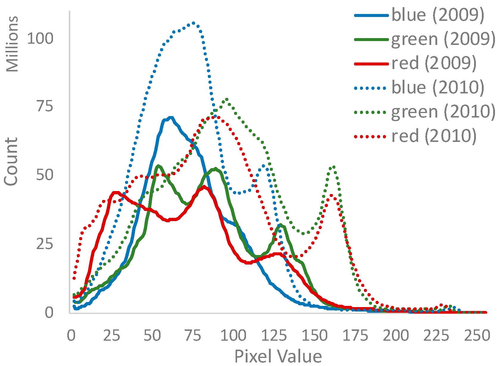
It is unclear why the 2009 aerial imagery consistently performed poorly compared to the 2010 aerial imagery. Analysis of the image pixel values for each of the colour channels (Figure 18) reveal different attributes for 2009 (solid) and 2010 (dashed). However, as augmentations were applied during training, the influence of this variation is likely to be minimal.
Additional research into data augmentations and data scaling may be needed to better represent the variations found in earth observation data.
The ability to identify PCS features over large geographical areas accelerated the mapping compilation of the national map for these regions. Mapping the current extent of PCS across Australia provides industry and stakeholders with essential baseline data that supports improved decision-making at multiple-scales, including the location and distribution of current production areas, and future opportunities for growth as well as preparing for and response to biosecurity incursions and naturals disasters which can adversely affect growers.
The final published map was informed using multiple sources of evidence including existing industry data, government land use mapping, remote sensing analytics, ground-based field surveys and citizen science enabled through web mapping applications. The map was built to the national standards of the ACLUMP coordinated by ABARES and is freely available. Privacy concerns are acknowledged and respected as no personal or confidential or commercial information is collected as a part of the mapping process nor contained within the mapping product.
5. Conclusions
This project demonstrates the methodology involved in building the first national map of PCS for Australia. The mapping was compiled using various sources of information including remote sensing data, ancillary data, field verification, industry data and engagement and deep learning analytics. Industry engagement was critical to ensure the map contained the information industry needed and it was fit for purpose. To encourage industry participation, a PCS Survey and Industry Engagement Web Application were developed which enabled peer review of the mapping product before it was published, which also support on-going updates to the map in future.
The results from the deep learning trials indicate that the use of computer vision technology can assist in the compilation of the PCS map. The outcomes of this research indicate that imagery with a spatial resolution of 50 cm is required to map PCS features accurately and can be applied to different sensors and geographical areas. The developed deep learning methods can identify greenhouse features to a high level of accuracy, but netting structures are more difficult to identify due to their transparent nature.
The models can identify PCS up to an accuracy of 0.94 when applied to a difference sensor type over a different geographical area. However, due to their transparent nature, net structures are difficult to identify within the imagery which caused some confusion within the models with some achieving an accuracy of <0.5. Mapping the greenhouses separately increased the accuracy to between 0.77 and 0.96. The KOMPSAT3 satellite imagery was the top performing sensor for detecting greenhouses and achieved a higher accuracy compared to the Skysat images, which could be the result of cloud contamination.
Despite the accuracy of the models, deep learning alone cannot be successfully used to create a national map of PCS to the level of accuracy required. However, with the assistance of deep learning, it is possible to expedite the compilation of the map and assist in identifying PCS features which may not easily be found over broad areas without the model output predictions.
Limitations of this approach is the requirement of high spatial resolution imagery and high computational resources (GPU). The method requires a high-quality training dataset. Extensive areas of PCS were mapped in South Australia and Queensland, allowing for the creation of deep learning models for this project. However, confusion within the netting class clearly caused issues.
Future work should focus on the maintenance and on-going update of the map. A modelling solution to identify new and removed structures will assist in ensuring the map remains current. Additional research should focus on refining the data augmentations to better represent the sensor, atmospheric and environmental differences between images.
Other potential work should include enhancement of the current mapping layer by working with Protected Cropping Australia and industry stakeholders to include additional information, such as crop/commodity type for individual features, and potentially other commercial information (e.g., ownership, productivity, etc.). This would be a larger project that secures both the on-going update of publicly available PCS map (dashboard) and an ‘industry only’ map for PCA only (as the industry body). AARSC have similar projects for the avocado, macadamia, banana and citrus horticulture tree crops funded by the industry bodies, Future Food Systems Cooperative Research Centre, Hort Innovation and UNE.
The success of the project resulted in the collaboration between industry, research and government. The support of industry bodies ensured the mapping outcomes were not perceived as an invasion of privacy and supported compilation of the map with access to existing industry data and their contribution through the industry engagement tools ensures ongoing validation of the mapping, both of which are integral to the accuracy and currency of the map. The spatial information generated by this project will assist ACLUMP and other jurisdictions when updating land use mapping in Australia.
The outcomes of this project offer significant benefit to the current ‘2030 road map for Protected Cropping in Australia’ being developed by Strategic Journeys for Food Innovation Australia Limited (FIAL), Macquarie Park, NSW, Australia and Queensland Department of Agriculture and Fisheries; as well as for the Hunger Map currently being developed by FoodBank Australia.
Author Contributions
Conceptualization, A.C., C.S. and J.M.; Methodology, A.C., C.S. and J.M.; Validation, A.C.; Formal analysis, A.C.; Data curation, A.C., C.S., R.B.M. and A.R. (Abbie Rankin); Writing—original draft, A.C.; Writing—review & editing, A.C., C.S., A.R. (Andrew Robson), J.M., R.B.M. and A.R. (Abbie Rankin); Visualization, A.C.; Supervision, A.R. (Andrew Robson); Project administration, C.S. and A.R. (Andrew Robson); Funding acquisition, A.R. (Andrew Robson). All authors have read and agreed to the published version of the manuscript.
Funding
The National Map of Protected Cropping Systems project is funded by the Hort Frontiers Advanced Production Systems Fund part of the Hort Frontiers strategic partnership initiative developed by Hort Innovation, with co-investment from Future Food Systems CRC, Protected Cropping Australia LTD, Greater Sydney and North Coast Local Land Services and the University of New England, and contributions from the Australian Government (AS20003).
Institutional Review Board Statement
Not applicable.
Informed Consent Statement
Not applicable.
Data Availability Statement
The National Map of Protected Cropping Structures can be accessed https://arcg.is/1CXbrW (accessed on 30 October 2023).
Acknowledgments
The project team acknowledge the funders of this project, that being the Future Food Systems CRC and Hort Innovation. The AARSC would also like to acknowledge the wider project team partners including Protected Cropping Australia (Matthew Plunkett and Sam Turner), NSW Local Land Services (Jonathan Eccles) for working so well together to achieve a common goal. The AARSC gratefully acknowledges the ongoing support from the respective industry bodies and the many growers and consultants that have collaborated on this project.
Conflicts of Interest
The authors declare no conflict of interest.
References
- Chakraborty, S.; Newton, A.C. Climate Change, Plant Diseases and Food Security: An Overview: Climate Change and Food Security. Plant Pathol. 2011, 60, 2–14. [Google Scholar] [CrossRef]
- Van Dijk, M.; Morley, T.; Rau, M.L.; Saghai, Y. A Meta-Analysis of Projected Global Food Demand and Population at Risk of Hunger for the Period 2010–2050. Nat. Food 2021, 2, 494–501. [Google Scholar] [CrossRef] [PubMed]
- Transforming Food Systems for Food Security, Improved Nutrition and Affordabel Healthy Diets for All. The State of Food Security and Nutrition in the World; FAO: Rome, Italy, 2021; ISBN 978-92-5-134325-8. [Google Scholar]
- United Nations Transforming Our World, the 2030 Agenda for Sustainable Development. General Assembly Resolution A/RES/70/1 2015; United Nations, Department of Economic and Social Affairs: New York, NY, USA, 2005. [Google Scholar]
- Rahaman, A.; Kumari, A.; Zeng, X.-A.; Khalifa, I.; Farooq, M.A.; Singh, N.; Ali, S.; Alee, M.; Aadil, R.M. The Increasing Hunger Concern and Current Need in the Development of Sustainable Food Security in the Developing Countries. Trends Food Sci. Technol. 2021, 113, 423–429. [Google Scholar] [CrossRef] [PubMed]
- Foodbank. Foodbank Hunger Report 2021-The Reality of the Food Crisis Facing Australia; Foodbank Australia Limited: North Ryde, NSW, Australia, 2021. [Google Scholar]
- Jensen, M.H.; Malter, A.J. Protected Agriculture: A Global Review; World Bank Technical Paper; World Bank: Washington, DC, USA, 1995; ISBN 978-0-8213-2930-6. [Google Scholar]
- Kumar, K.S.; Tiwari, K.N.; Jha, M.K. Design and Technology for Greenhouse Cooling in Tropical and Subtropical Regions: A Review. Energy Build. 2009, 41, 1269–1275. [Google Scholar] [CrossRef]
- Vuković, M.; Jurić, S.; Maslov Bandić, L.; Levaj, B.; Fu, D.-Q.; Jemrić, T. Sustainable Food Production: Innovative Netting Concepts and Their Mode of Action on Fruit Crops. Sustainability 2022, 14, 9264. [Google Scholar] [CrossRef]
- Thackway, R. (Ed.) Land Use in Australia; ANU Press: Acton, ACT, Australia, 2018; ISBN 978-1-921934-42-1. [Google Scholar]
- Lambin, E.F.; Tran, A.; Vanwambeke, S.O.; Linard, C.; Soti, V. Pathogenic Landscapes: Interactions between Land, People, Disease Vectors, and Their Animal Hosts. Int. J. Health Geogr. 2010, 9, 54. [Google Scholar] [CrossRef] [PubMed]
- Anyamba, A.; Small, J.L.; Britch, S.C.; Tucker, C.J.; Pak, E.W.; Reynolds, C.A.; Crutchfield, J.; Linthicum, K.J. Recent Weather Extremes and Impacts on Agricultural Production and Vector-Borne Disease Outbreak Patterns. PLoS ONE 2014, 9, e92538. [Google Scholar] [CrossRef] [PubMed]
- Stoddard, S.T.; Morrison, A.C.; Vazquez-Prokopec, G.M.; Paz Soldan, V.; Kochel, T.J.; Kitron, U.; Elder, J.P.; Scott, T.W. The Role of Human Movement in the Transmission of Vector-Borne Pathogens. PLoS Negl. Trop. Dis. 2009, 3, e481. [Google Scholar] [CrossRef] [PubMed]
- Chawla, I.; Karthikeyan, L.; Mishra, A.K. A Review of Remote Sensing Applications for Water Security: Quantity, Quality, and Extremes. J. Hydrol. 2020, 585, 124826. [Google Scholar] [CrossRef]
- Karthikeyan, L.; Chawla, I.; Mishra, A.K. A Review of Remote Sensing Applications in Agriculture for Food Security: Crop Growth and Yield, Irrigation, and Crop Losses. J. Hydrol. 2020, 586, 124905. [Google Scholar] [CrossRef]
- Jiménez-Lao, R.; Aguilar, F.J.; Nemmaoui, A.; Aguilar, M.A. Remote Sensing of Agricultural Greenhouses and Plastic-Mulched Farmland: An Analysis of Worldwide Research. Remote Sens. 2020, 12, 2649. [Google Scholar] [CrossRef]
- Koc-San, D. Evaluation of Different Classification Techniques for the Detection of Glass and Plastic Greenhouses from WorldView-2 Satellite Imagery. J. Appl. Remote Sens. 2013, 7, 073553. [Google Scholar] [CrossRef]
- Tarantino, E.; Figorito, B. Mapping Rural Areas with Widespread Plastic Covered Vineyards Using True Color Aerial Data. Remote Sens. 2012, 4, 1913–1928. [Google Scholar] [CrossRef]
- Arcidiacono, C.; Porto, S.M.C. A Model to Manage Crop-Shelter Spatial Development by Multi-Temporal Coverage Analysis and Spatial Indicators. Biosyst. Eng. 2010, 107, 107–122. [Google Scholar] [CrossRef]
- Vox, G.; Loisi, R.V.; Blanco, I.; Mugnozza, G.S.; Schettini, E. Mapping of Agriculture Plastic Waste. Agric. Agric. Sci. Procedia 2016, 8, 583–591. [Google Scholar] [CrossRef]
- Blanco, I.; Loisi, R.V.; Sica, C.; Schettini, E.; Vox, G. Agricultural Plastic Waste Mapping Using GIS. A Case Study in Italy. Resour. Conserv. Recycl. 2018, 137, 229–242. [Google Scholar] [CrossRef]
- Parlato, M.C.M.; Valenti, F.; Porto, S.M.C. Covering Plastic Films in Greenhouses System: A GIS-Based Model to Improve Post Use Suistainable Management. J. Environ. Manag. 2020, 263, 110389. [Google Scholar] [CrossRef] [PubMed]
- Picuno, P.; Tortora, A.; Capobianco, R.L. Analysis of Plasticulture Landscapes in Southern Italy through Remote Sensing and Solid Modelling Techniques. Landsc. Urban Plan. 2011, 100, 45–56. [Google Scholar] [CrossRef]
- Aguilar, M.; Nemmaoui, A.; Novelli, A.; Aguilar, F.; García Lorca, A. Object-Based Greenhouse Mapping Using Very High Resolution Satellite Data and Landsat 8 Time Series. Remote Sens. 2016, 8, 513. [Google Scholar] [CrossRef]
- Ou, C.; Yang, J.; Du, Z.; Liu, Y.; Feng, Q.; Zhu, D. Long-Term Mapping of a Greenhouse in a Typical Protected Agricultural Region Using Landsat Imagery and the Google Earth Engine. Remote Sens. 2019, 12, 55. [Google Scholar] [CrossRef]
- Chen, Z.; Wu, Z.; Gao, J.; Cai, M.; Yang, X.; Chen, P.; Li, Q. A Convolutional Neural Network for Large-Scale Greenhouse Extraction from Satellite Images Considering Spatial Features. Remote Sens. 2022, 14, 4908. [Google Scholar] [CrossRef]
- Ma, A.; Chen, D.; Zhong, Y.; Zheng, Z.; Zhang, L. National-Scale Greenhouse Mapping for High Spatial Resolution Remote Sensing Imagery Using a Dense Object Dual-Task Deep Learning Framework: A Case Study of China. ISPRS J. Photogramm. Remote Sens. 2021, 181, 279–294. [Google Scholar] [CrossRef]
- Clark, A.; McKechnie, J. Detecting Banana Plantations in the Wet Tropics, Australia, Using Aerial Photography and U-Net. Appl. Sci. 2020, 10, 2017. [Google Scholar] [CrossRef]
- Yin, L.; Ghosh, R.; Lin, C.; Hale, D.; Weigl, C.; Obarowski, J.; Zhou, J.; Till, J.; Jia, X.; You, N.; et al. Mapping Smallholder Cashew Plantations to Inform Sustainable Tree Crop Expansion in Benin. Remote Sens. Environ. 2023, 295, 113695. [Google Scholar] [CrossRef]
- Australian Bureau of Agricultural and Resource Economics and Sciences. The Australian Land Use and Management Classification Version 8; Australian Bureau of Agricultural and Resource Economics and Sciences: Canberra, ACT, Australia, 2016.
- Australian Bureau of Agricultural Resource Economics and Sciences (ABARES). Catchment Scale Land Use of Australia—Update December 2020; ABARES: Canberra, ACT, Australia, 2021.
- Ronneberger, O.; Fischer, P.; Brox, T. U-Net: Convolutional Networks for Biomedical Image Segmentation. arXiv 2015, arXiv:1505.04597. [Google Scholar]
- Voulodimos, A.; Doulamis, N.; Doulamis, A.; Protopapadakis, E. Deep Learning for Computer Vision: A Brief Review. Comput. Intell. Neurosci. 2018, 2018, 7068349. [Google Scholar] [CrossRef] [PubMed]
- Clark, A.; Phinn, S.; Scarth, P. Optimised U-Net for Land Use–Land Cover Classification Using Aerial Photography. PFG—J. Photogramm. Remote Sens. Geoinf. Sci. 2023, 91, 125–147. [Google Scholar] [CrossRef]
- Clark, A.; Phinn, S.; Scarth, P. Pre-Processing Training Data Improves Accuracy and Generalisability of Convolutional Neural Network Based Landscape Semantic Segmentation. Land 2023, 12, 1268. [Google Scholar] [CrossRef]
- Dosovitskiy, A.; Springenberg, J.T.; Brox, T. Unsupervised Feature Learning by Augmenting Single Images. arXiv 2013, arXiv:1312.5242v3. [Google Scholar]
- Wieland, M.; Li, Y.; Martinis, S. Multi-Sensor Cloud and Cloud Shadow Segmentation with a Convolutional Neural Network. Remote Sens. Environ. 2019, 230, 111203. [Google Scholar] [CrossRef]
- Kattenborn, T.; Leitloff, J.; Schiefer, F.; Hinz, S. Review on Convolutional Neural Networks (CNN) in Vegetation Remote Sensing. ISPRS J. Photogramm. Remote Sens. 2021, 173, 24–49. [Google Scholar] [CrossRef]
- Sun, Y.; Tian, Y.; Xu, Y. Problems of Encoder-Decoder Frameworks for High-Resolution Remote Sensing Image Segmentation: Structural Stereotype and Insufficient Learning. Neurocomputing 2019, 330, 297–304. [Google Scholar] [CrossRef]
- Davis, J.; Goadrich, M. The Relationship between Precision-Recall and ROC Curves. In Proceedings of the 23rd international conference on Machine learning-ICML ’06, Pittsburgh, PA, USA, 25–29 June 2006; ACM Press: New York, NY, USA, 2006; pp. 233–240. [Google Scholar]
Figure 1.
Hierarchical classification for Protected Cropping Systems.

Figure 2.
PCS Structure classes. Imagery © Maxar; Map data © OpenStreetMap contributors (Esri Basemaps); and street-view imagery © Google Maps.
Figure 2.
PCS Structure classes. Imagery © Maxar; Map data © OpenStreetMap contributors (Esri Basemaps); and street-view imagery © Google Maps.

Figure 3.
Temporary netting example including 2022 (a) and 2023 aerial imagery (b) PCS mapping (c) and ground view (d). (138°52′30″ E 34°58′34″ S) Imagery © Maxar; Map data © OpenStreetMap contributors (Esri Basemaps); and Street-view imagery © Google Maps.
Figure 3.
Temporary netting example including 2022 (a) and 2023 aerial imagery (b) PCS mapping (c) and ground view (d). (138°52′30″ E 34°58′34″ S) Imagery © Maxar; Map data © OpenStreetMap contributors (Esri Basemaps); and Street-view imagery © Google Maps.
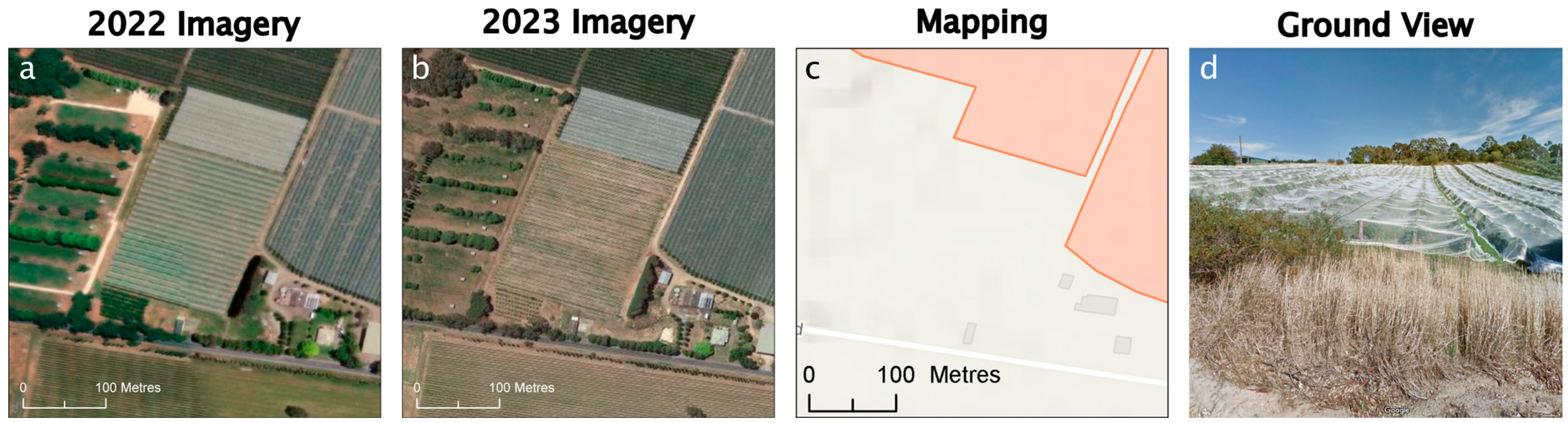
Figure 5.
PCS field validation GPS tracks across Australia.

Figure 6.
PCS mapping (a) and on-ground field observation (b) at, Hillwood Berry Farm, Tamar Valley, Tasmania. The red ‘x’ in (a) represents the location of field observation in (b).
Figure 6.
PCS mapping (a) and on-ground field observation (b) at, Hillwood Berry Farm, Tamar Valley, Tasmania. The red ‘x’ in (a) represents the location of field observation in (b).

Figure 7.
Example of randomly applied augmentation combinations over an area consisting of protected cropping structures including the original image (a) and three augmented versions (b–d). Note these examples do not represent the patch size used in this study.
Figure 7.
Example of randomly applied augmentation combinations over an area consisting of protected cropping structures including the original image (a) and three augmented versions (b–d). Note these examples do not represent the patch size used in this study.
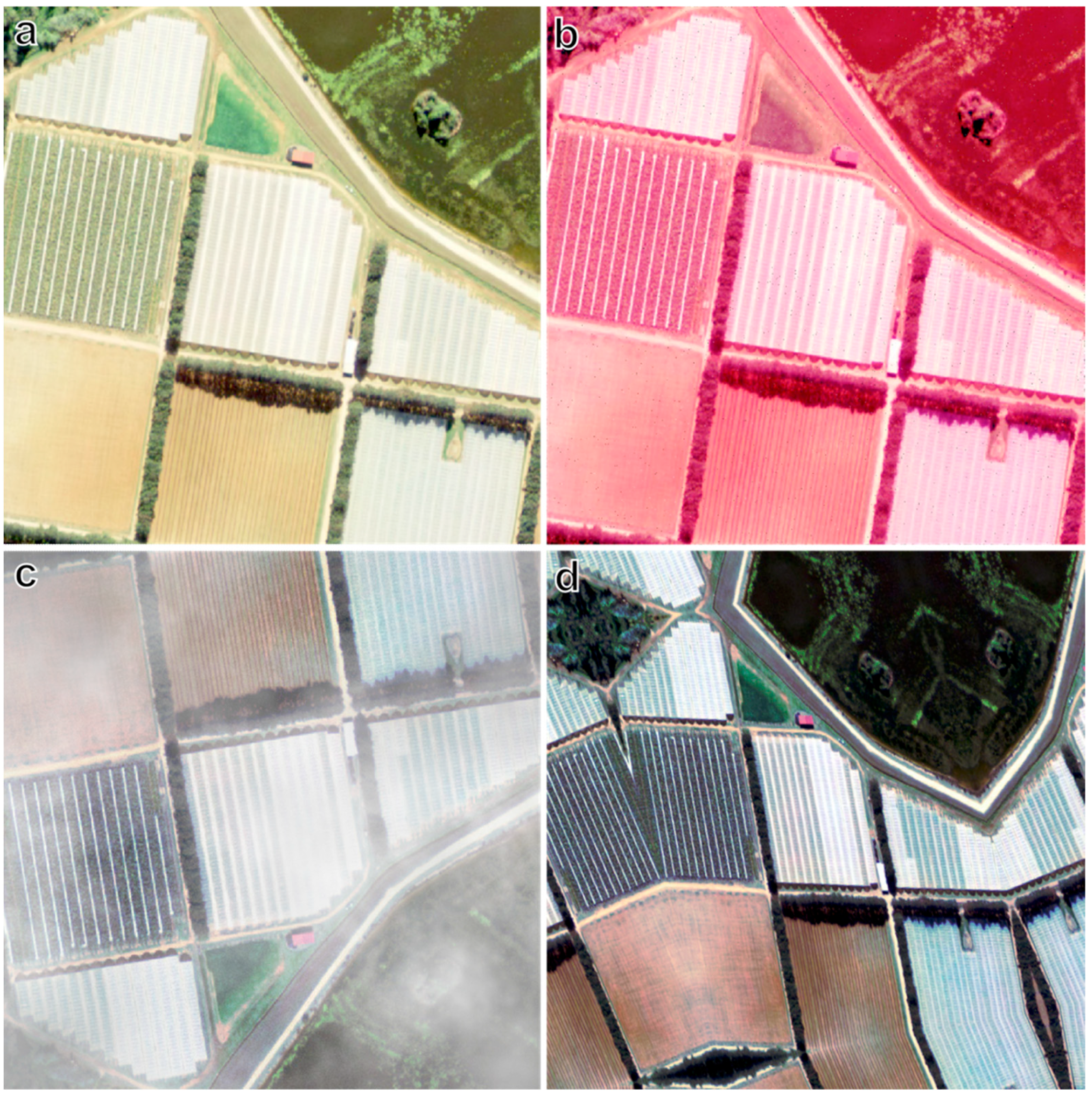
Figure 8.
Training imagery for Greater Adelaide (a) and Southeast Queensland (b).
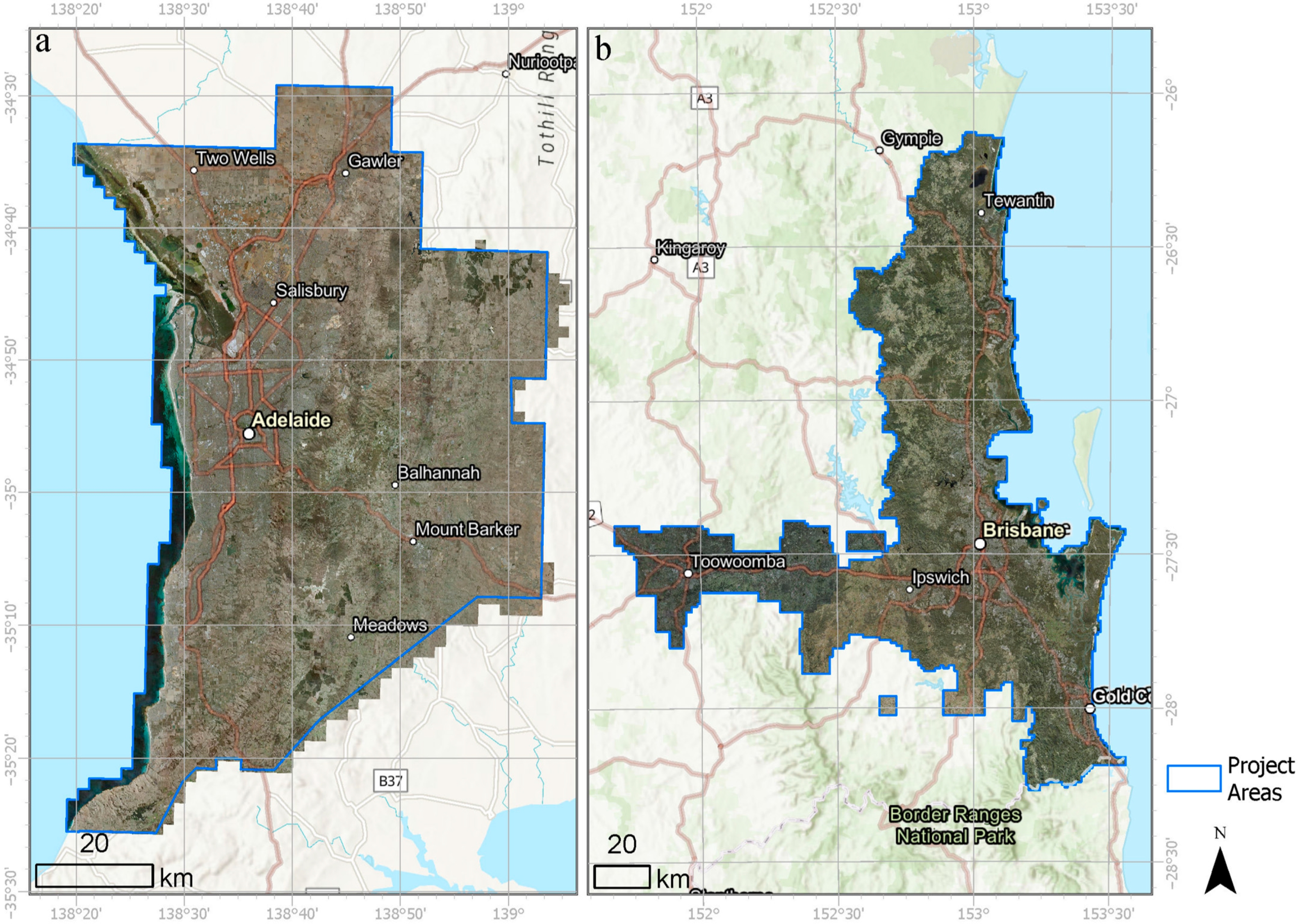
Figure 9.
Example of the spatial distribution of training patches in Redlands, South East Queensland.
Figure 9.
Example of the spatial distribution of training patches in Redlands, South East Queensland.
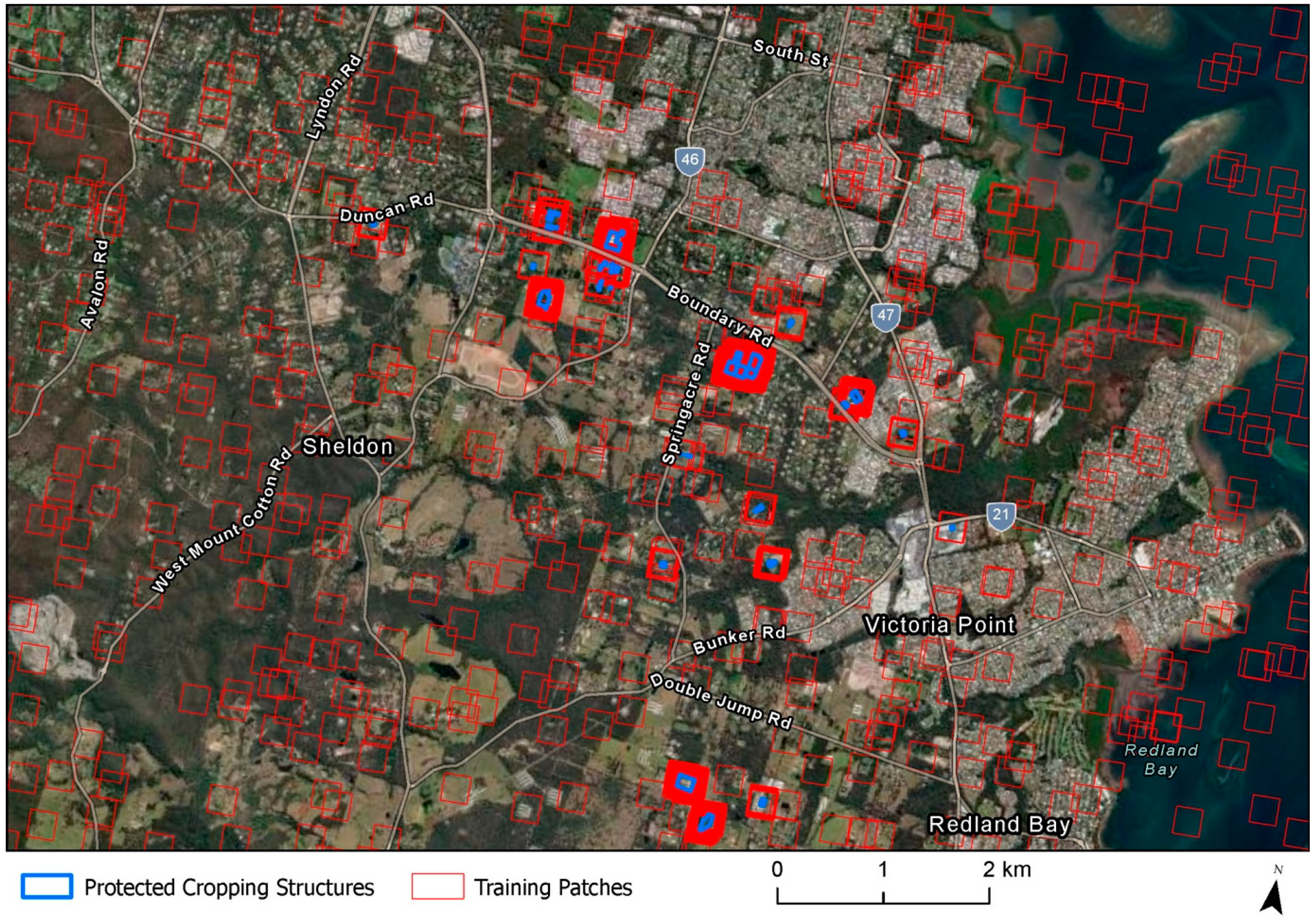
Figure 10.
Australian protected cropping systems modelling project areas of Southeast Queensland (a); Greater Adelaide (b) and Dirty Creek (c).
Figure 10.
Australian protected cropping systems modelling project areas of Southeast Queensland (a); Greater Adelaide (b) and Dirty Creek (c).
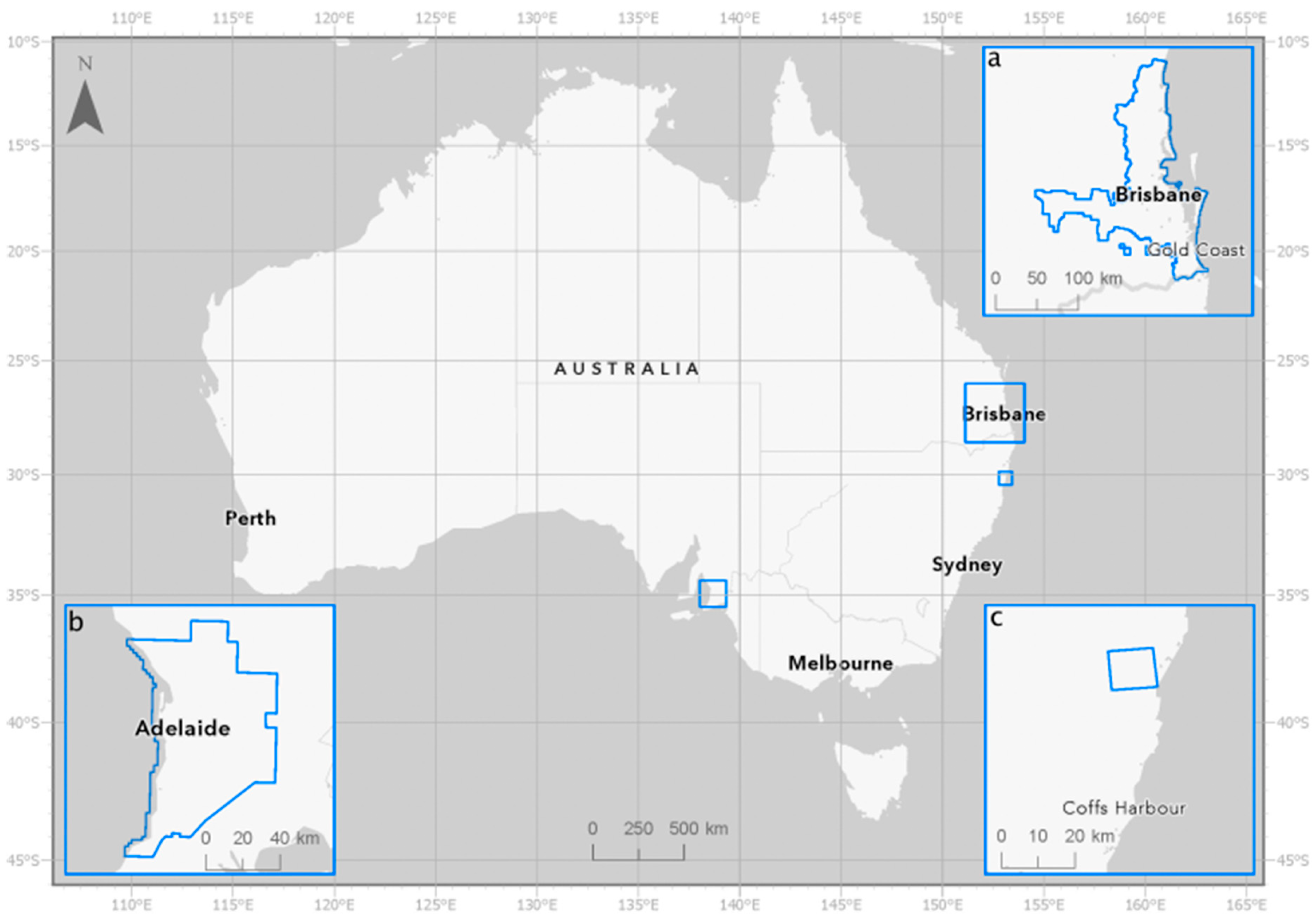
Figure 11.
Protected cropping systems validation imagery near Dirty Creek, New South Wales including training data (a), 2009 aerial imagery (b), 2010 aerial imagery (c), 2023 Skysat satellite imagery 1 (d), 2023 Skysat satellite imagery 2 (e), 2022 KOMPSAT3 satellite imagery (f).
Figure 11.
Protected cropping systems validation imagery near Dirty Creek, New South Wales including training data (a), 2009 aerial imagery (b), 2010 aerial imagery (c), 2023 Skysat satellite imagery 1 (d), 2023 Skysat satellite imagery 2 (e), 2022 KOMPSAT3 satellite imagery (f).

Figure 12.
Coverage of aerial photography the computer model was applied including: 2018 Greater Sydney (a); 2021 North Queensland (b); 2019 Central Queensland (c); 2021 Capricornia and Wide Bay (d); and 2020 Southern Wide Bay (e). The colours represent the extent of each regional image capture.
Figure 12.
Coverage of aerial photography the computer model was applied including: 2018 Greater Sydney (a); 2021 North Queensland (b); 2019 Central Queensland (c); 2021 Capricornia and Wide Bay (d); and 2020 Southern Wide Bay (e). The colours represent the extent of each regional image capture.
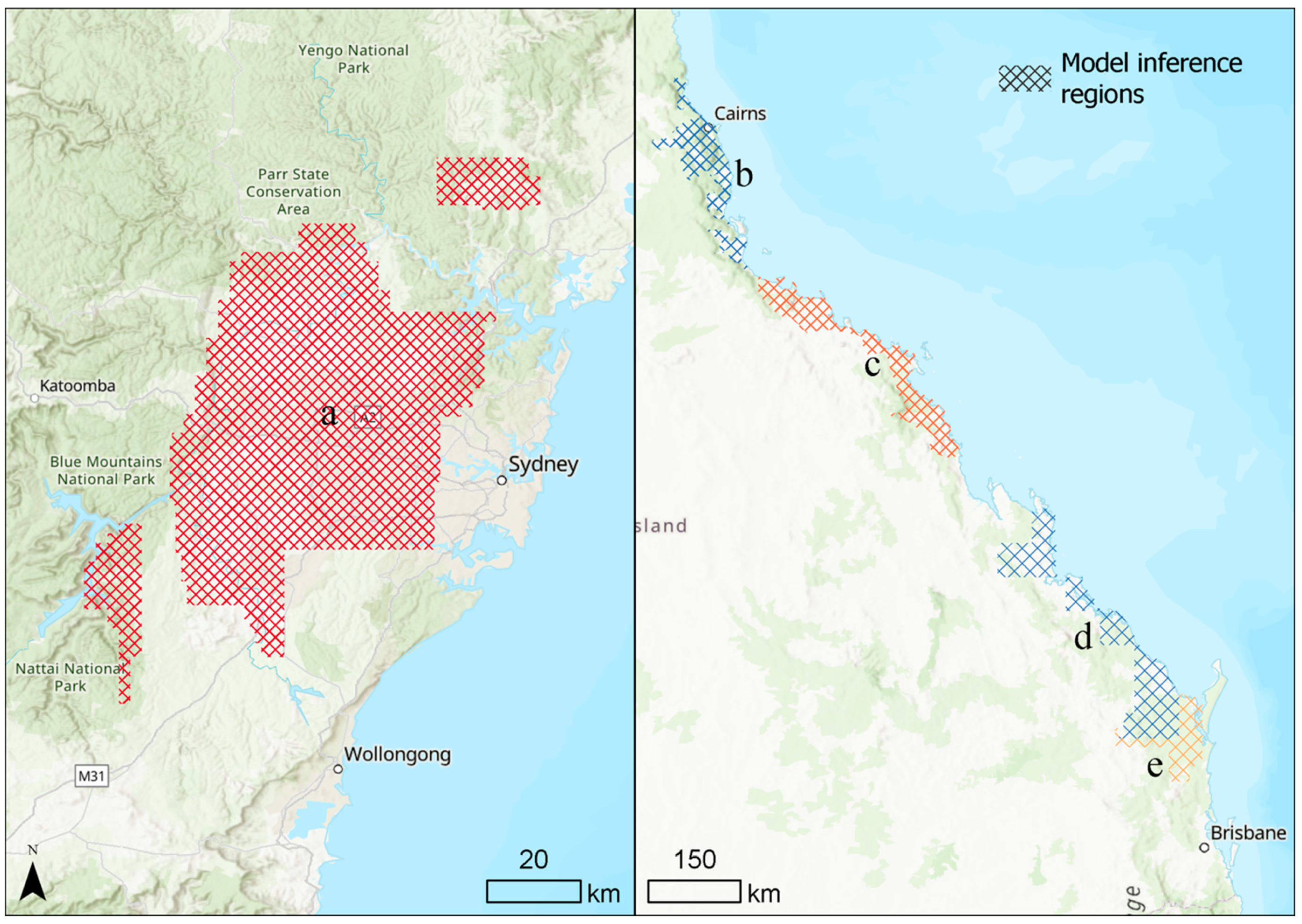
Figure 13.
PCS structure features as mapped in edit layer (a) and the derived mapping product as published (b).
Figure 13.
PCS structure features as mapped in edit layer (a) and the derived mapping product as published (b).

Figure 14.
Box and whisker plots displaying the results from the spatial resolution experiment. For each spatial resolution, five models were trained on Southeast Queensland PCS data and validated on Adelaide PCS data. The F1-Score value indicates the accuracy of each model. For each spatial resolution plot, the range of accuracies are represented by the lines and the box shows the quartiles of the resolution accuracy.
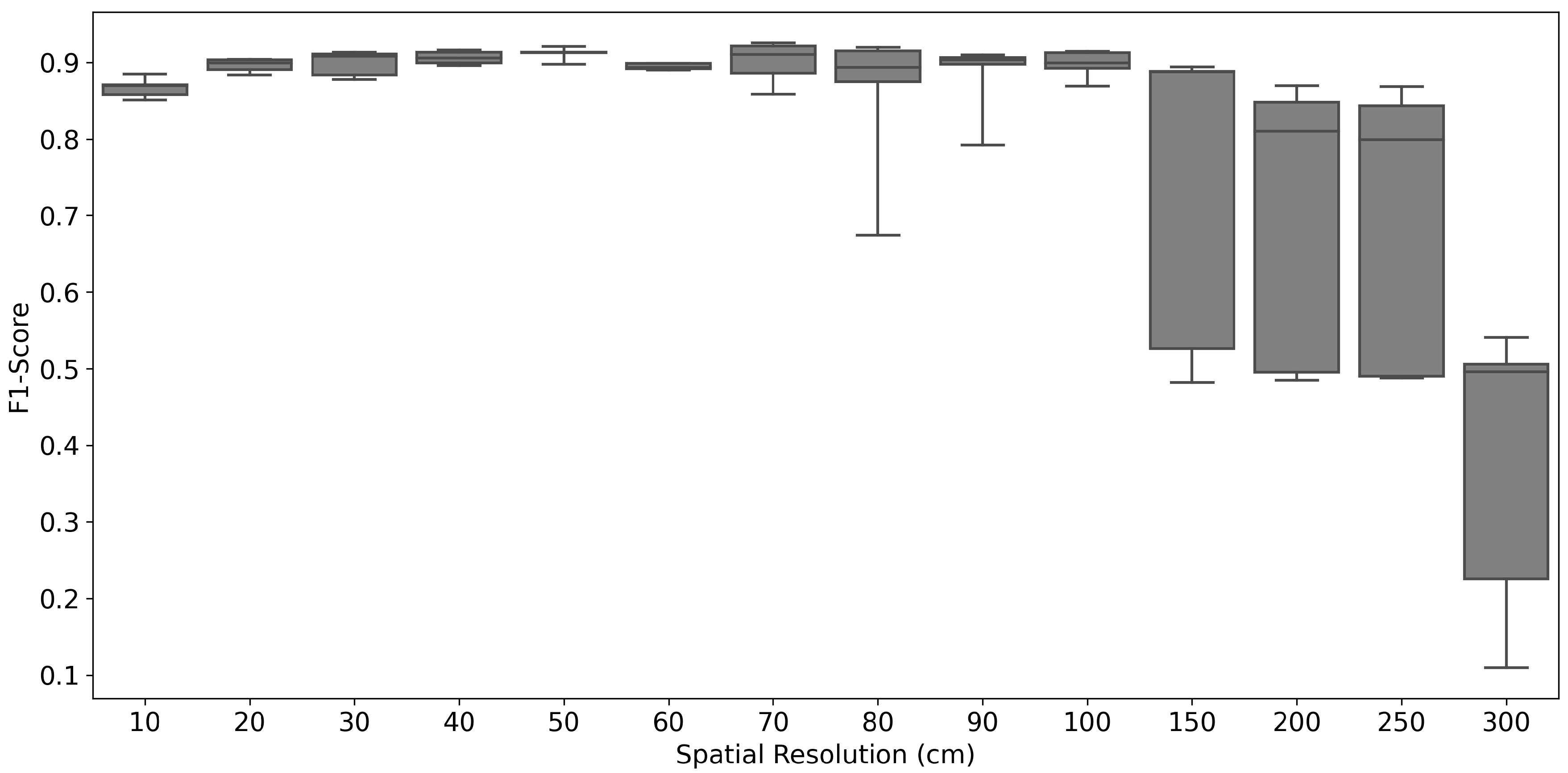
Figure 15.
Results from the PCS class trials including all protected cropping systems (a), greenhouses (b) and nets (c). a2009 and a2010 represent the aerial photography for 2009 and 2010, respectively, ks represent KOMPSAT3 satellite imagery and ss1 and ss2 the two Skysat satellite images. For each imagery type, the range of accuracies are represented by the lines, the box shows the quartiles and the ‘♦’ symbol outliers.
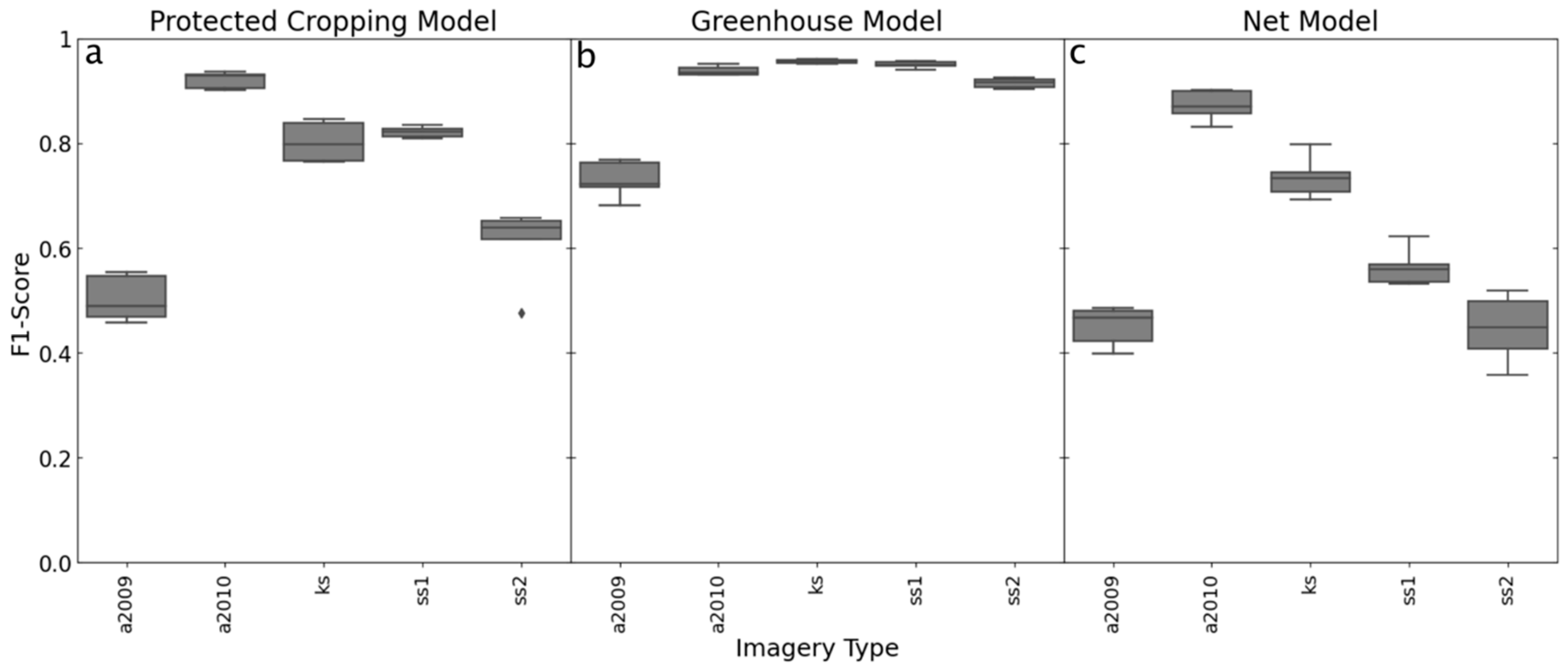
Figure 16.
Protected Cropping Systems model output classifications showing ground-truth data, protected cropping systems model, greenhouses model and nets model. The blue shading represents the model confidence with light blue indicating a low probability and dark blue a high probability of the target feature type.

Figure 17.
PCS structure type area.

Figure 18.
Image histogram for 2009 (solid) and 2010 (dashed) for the red, green and blue colour channels.
Figure 18.
Image histogram for 2009 (solid) and 2010 (dashed) for the red, green and blue colour channels.

Table 1.
PCS structure production area by state/territory.
| State/Territory | Glasshouse (ha) | Polyhouse (ha) | Polytunnel (ha) | Net (ha) | Shadehouse (ha) | Total (ha) |
|---|---|---|---|---|---|---|
| ACT | 0 | 0 | 0 | 1 | 3 | 4 |
| New South Wales | 57 | 384 | 649 | 3005 | 120 | 4216 |
| Northern Territory | 0 | 0 | 1 | 73 | 12 | 86 |
| Queensland | 5 | 292 | 399 | 1872 | 130 | 2698 |
| South Australia | 87 | 1103 | 22 | 816 | 20 | 2048 |
| Tasmania | 9 | 7 | 505 | 803 | 0 | 1323 |
| Victoria | 125 | 166 | 354 | 1925 | 29 | 2598 |
| Western Australia | 9 | 49 | 249 | 532 | 118 | 958 |
| Total | 293 | 2001 | 2180 | 9028 | 431 | 13,932 |
Disclaimer/Publisher’s Note: The statements, opinions and data contained in all publications are solely those of the individual author(s) and contributor(s) and not of MDPI and/or the editor(s). MDPI and/or the editor(s) disclaim responsibility for any injury to people or property resulting from any ideas, methods, instructions or products referred to in the content. |
© 2023 by the authors. Licensee MDPI, Basel, Switzerland. This article is an open access article distributed under the terms and conditions of the Creative Commons Attribution (CC BY) license (https://creativecommons.org/licenses/by/4.0/).
Share and Cite
MDPI and ACS Style
Clark, A.; Shephard, C.; Robson, A.; McKechnie, J.; Morrison, R.B.; Rankin, A. A Multifaceted Approach to Developing an Australian National Map of Protected Cropping Structures. Land 2023, 12, 2168. https://doi.org/10.3390/land12122168
AMA Style
Clark A, Shephard C, Robson A, McKechnie J, Morrison RB, Rankin A. A Multifaceted Approach to Developing an Australian National Map of Protected Cropping Structures. Land. 2023; 12(12):2168. https://doi.org/10.3390/land12122168
Chicago/Turabian StyleClark, Andrew, Craig Shephard, Andrew Robson, Joel McKechnie, R. Blake Morrison, and Abbie Rankin. 2023. "A Multifaceted Approach to Developing an Australian National Map of Protected Cropping Structures" Land 12, no. 12: 2168. https://doi.org/10.3390/land12122168
Note that from the first issue of 2016, this journal uses article numbers instead of page numbers. See further details here.