
Extrapolation of Digital Soil Mapping Approaches for Soil Organic Carbon Stock Predictions in an Afromontane Environment


1
Department of Soil, Crop, and Climate Sciences, University of the Free State, Bloemfontein 9301, South Africa
2
Afromontane Research Unit, Department of Geography, University of the Free State, Qwaqwa Campus, Private Bag X13, Phuthaditjhaba 9866, South Africa
*
Author to whom correspondence should be addressed.
Land 2023, 12(3), 520; https://doi.org/10.3390/land12030520
Submission received: 21 January 2023
/
Revised: 8 February 2023
/
Accepted: 15 February 2023
/
Published: 21 February 2023
Abstract
:Soil scientists can aid in an essential part of ecological conservation and rehabilitation by quantifying soil properties, such as soil organic carbon (SOC), and is stock (SOCs) SOC is crucial for providing ecosystem services, and, through effective C-sequestration, the effects of climate change can be mitigated. In remote mountainous areas with complex terrain, such as the northern Maloti-Drakensberg in South Africa and Lesotho, direct quantification of stocks or even obtaining sufficient data to construct predictive Digital Soil Mapping (DSM) models is a tedious and expensive task. Extrapolation of DSM model and algorithms from a relatively accessible area to remote areas could overcome these challenges. The aim of this study was to determine if calibrated DSM models for one headwater catchment (Tugela) can be extrapolated without re-training to other catchments in the Maloti-Drakensberg region with acceptable accuracy. The selected models were extrapolated to four different headwater catchments, which included three near the Motete River (M1, M2, and M3) in Lesotho and one in the Vemvane catchment adjacent to the Tugela. Predictions were compared to measured stocks from the soil sampling sites (n = 98) in the various catchments. Results showed that based on the mean results from Universal Kriging (R2 = 0.66, NRMSE = 0.200, and ρc = 0.72), least absolute shrinkage and selection operator or LASSO (R2 = 0.67, NRMSE = 0.191, and ρc = 0.73) and Regression Kriging with cubist models (R2 = 0.61, NRMSE = 0.184, and ρc = 0.65) had the most satisfactory outcome, whereas the soil-land inference models (SoLIM) struggled to predict stocks accurately. Models in the Vemvane performed the worst of all, showing that that close proximity does not necessarily equal good similarity. The study concluded that a model calibrated in one catchment can be extrapolated. However, the catchment selected for calibration should be a good representation of the greater area, otherwise a model might over- or under-predict SOCs. Successfully extrapolating models to remote areas will allow scientists to make predictions to aid in rehabilitation and conservation efforts of vulnerable areas.
1. Introduction
Soil has a multifunctional role within the ecosystem [1], such as water filtration, serves as a habitat for microorganisms, growing medium for plants, and ensures good biodiversity under the right circumstances. Quantifying soil properties and their spatial distribution are essential in ecological conservation and rehabilitation. Soil organic carbon (SOC) is likely the soil property that has received most attention in recent years. SOC is a valuable resource regarding ecosystem services and, therefore, is an effective indicator to determine soil degradation/health status [2]. However, The SOC concentration varies strongly among different climatic conditions, land use practices [3], biomes, and even within a specified biome.
Grassland biomes contain up to 30% of the world’s carbon [4], and occupy around 40% of the Earth’s landmass, thus it can be considered as critical performers in C cycling [5]. A decrease in these biomes’ sequestration capacity can result in substantial changes in the global C-budget [4]. Correct management of grasslands can have a significant impact on mitigating climate change through enhanced sequestration, but degradation can result in considerable losses of sequestered carbon to the atmosphere [6].
In Southern Africa, the alpine areas of the Maloti-Drakensberg have some of the highest SOC concentrations of the region. These carbon hotspots are being degraded, mostly due to mismanagement of livestock [7]. There is a need to quantify these stocks and their spatial distribution in the area in order to preserve them. However, the complex terrain of the Maloti-Drakensberg region presents a challenging task to conduct conventional soil surveys. This is due to the limited accessible roads, very steep terrain, and the high elevation (>3000 m.a.s.l.). Digital soil mapping (DSM) is proposed as a cost-effective alternative to conventional soil mapping, especially in remote areas [8]. With DSM, soil properties could be map if relationships between these properties and their environment could be established through the use of predictive statistics or geo-statistics [9,10]. In the recent past, numerous studies have successfully predicted the spatial distribution of SOC in various environments [11,12,13,14,15]. Other studies focused on the potential of constructing DSM models in one area and extrapolating these to other locations [16,17].
Here, we also focussed on the potential of different DSM models to be extrapolated alpine areas of the northern Maloti-Drakensberg. Mapping the entire alpine region of the Maloti-Drakensberg at adequate scale will be very costly and time-consuming as very few areas are readily accessible. Therefore, the overall aim was to determine if previously calibrated models for SOC prediction [18] in a relatively accessible area (Tugela headwater catchment) can predict SOC stocks in other areas without re-training the models. Specific objectives were to sample and quantify soil organic carbon stocks (SOCs) of new catchments in the region using DSM techniques, and statistical comparison of the accuracy of the models to determine the best suited for extrapolation.
2. Materials and Methods
2.1. Study Area
This study was conducted in headwater catchments in the northern Maloti-Drakensberg region. The Tugela headwater catchment (300-ha) includes Mont-Aux Sources (3282 m.a.s.l.) and the Tugela Falls (2973 m.a.s.l.), and is situated near borders of Lesotho, KwaZulu-Natal, and the Free State provinces. This catchment was the focus of a DSM study [18] and served as ‘training ground’ from which the models were extrapolated. The four focus catchments in the current study were named Vemvane (28°45′13.0″ S, 28°52′16.0″ E), M1 (28°51′23.9″ S, 28°46′55.7″ E), M2 (28°52′49.3″ S, 28°48′17.7″ E), and M3 (28°53′46.9″ S, 28°47′30.6″ E), based on the rivers running through them (‘M’ is for the Motete River). All four study catchments are situated above 3000 m.a.s.l. with the highest point reaching 3319 m.a.s.l. in the M1 catchment. The Vemvane (145 ha) catchment is situation next to the Tugela headwater catchment in the Free State’s border, whereas the M1 (189 ha), M2 (132 ha), and M3 (192 ha) catchments are within Lesotho’s borders next to the A1 national road (Figure 1).
All four catchments have montane wetlands in the footslope and hillslopes as seeps. The catchments boasted a range of soil types, which included Leptic Fibric- and Leptic Sapric-Histosols, Chernic-, Umbric-, Dystric-, and Cutanic-Leptosols. The soil profiles in the valley bottom are saturated with water for long periods of time. The area has a grassy ecosystem [19], which is frequently visited by grazing animals. Ice rats, Otomys sloggetti robertsi, also inhabit the alpine areas of northern Lesotho [20], where they make their burrows in the ground; however, there were no sightings in the Vemvane. The area falls within a cool, wet, summer rainfall region, with cold winters where the surface is covered in frost. The rainfall for the Vemvane catchment is estimated to be between 1200–1500 mm, whereas the Motete catchments are considered to experience an annual rainfall of >1500 mm [21]. The geology of the larger area can be considered to form part of the Drakensberg group that consists of mainly basalt and non-intrusive dolerite [22].
2.2. Mapping and Modeling Methods
The same models were used for extrapolation, and was calibrated by using only samples gathered in the Tugela headwater catchment. Thus, SOCs from the Tugela (90 sampling sites) were divided into an 80% calibration and 20% validation ratio. The Tugela validation data was not added back to the calibration data when extrapolated to ensure that the models remained the same after they were calibrated. The models that were extrapolated included SoLIM rule-based and sample-based methods (SoLIM-RB and SoLIM-SB), random forest (RF), least absolute shrinkage and selection operator (LASSO), regression Kriging with cubist (RK-CB), and universal Kriging (UK).
For the other headwater catchments, all the samples gathered within each area were solely used for testing and not training. The models were therefore not recalibrated and used as is to assess if they could be used for extrapolation.
2.2.1. SoLIM Rule-Based
SoLIMSolutions 2015 were used to create both SoLIM rule-based (SoLIM-RB) and sample-based (SoLIM-SB) maps. With SoLIM-RB, a single hardened map is generated containing a combined map of all soil associations that is a function of fuzzy membership maps obtained through soil associations. This approach is usually best suited for mapping categorical data; however, continuous soil properties can also be mapped by combining the soil association distribution with mean or typical values of the soil property [23].
The soil samples from the Tugela were classified into five groups: organic, shallow humic profiles (Hs), deep humic profiles (Hd), deep orthic profiles (Od), and shallow orthic profiles (Os) [18]. The expert knowledge approach was used to link the five soil groups to their respective positions in the landscape. The rules assigned to each soil group (Table 1) in order to extract fuzzy membership maps that lead to the SoLIM-RB map was kept the same for the extrapolation process.
The goal for these rules was to assign a range of values where an environmental variable is more optimal for a soil group, i.e., where high optimal values occur there is a strong relationship or similarity for a specific group to occur [24].
2.2.2. SoLIM Sample-Based
SoLIM-SB makes use of sampled/measured values gathered from the field rather than rules formulated by the expert [24]. The method assumes that sampling locations that have similar or close to similar environmental conditions would have similar soil property values [15]. Thus, SoLIM can predict the soil properties, such as SOCs of a location by assigning similar or close to similar values based on the environmental covariates and their similarities to observed properties [15,24].
2.2.3. Random Forest
The Random Forest (RF) algorithm is based on bagging (ensemble learning), which entails aggregating a large number of trees (predictions) into one by streamlining it into an average of the individual tree [12,13,25]. By generating multiple trees, RF can perform both classification and regression [13,25]. This can enhance prediction accuracy by reducing experimental noise [12]. To map SOCs, the RF model has three main parameters that required tuning during the training phase. The parameters were ntree (the number of trees), mtry (the number of variables used to construct each tree), and nodesize (the minimum number of nodes for each tree). In order to successfully model with RF, the mtry parameter can be considered especially important and should be considered with particular understanding [13]. For this study, the mtry parameter was determined through the caret package using the randomForest algorithm.
2.2.4. Least Absolute Shrinkage and Selection Operator
LASSO (least absolute shrinkage and selection operator) can be used for selecting the important covariates by eliminating non-relevant predictors [26]. Similar to elastic net and ridge regression, LASSO is based on least squares regression. However, it introduces a penalized residual sum of squares, with the penalty being equal to the weighted sum of absolute values of the estimated coefficients [26,27]. The penalty value (λ) is what separates it from a normal least square regression and is the major parameter that should be carefully calculated when training the model. Using cross-validation allowed for finding the optimal λ value by considering the increase or decrease in error, by referring to the RMSE value associated with the corresponding λ value. The glmnet algorithm through the caret package was used for cross-validation, where resampling through an 8-fold cross repeated 10 times was done.
2.2.5. Regression Kriging with Cubist Models
Regression kriging with cubist (RK-CB) is a hybrid approach that entails a cubist model combined with the kriged residuals to produce a single map [25]. On its own the cubist model is remarkably similar to regression trees, such as the RF model, where it can perform observations of linear and non-linear relationships through a data partitioning algorithm [13,25,26]. It divides the data up into subsets with similar characteristics to the target variable and covariates rather than using the whole dataset at once [12]. Regression kriging uses a combination of a regression from the soil property on covariates and the Kriged residuals of the soil property [28]. Through the use of regression Kriging the CB-RK model is an effective method for predicting the spatial distribution of soil properties.
For the cubist part of the hybrid model, the cubistControl parameter in the Cubist package is considered the main parameter. It includes the number of rules, committees, and extrapolation (expressed as percentage). For the regression Kriging part, it is essential that the coordinate reference system (CRS) for point data and the covariates are identical. The variogram should then be fitted to find the optimal model, nugget, sill, and range values. The variogram function in the automap algorithm served as an essential part for fitting the variogram for any model structure. The residual kriging model was done through the gstat package. Lastly, the cubist model and regression Kriging model was combined to form the RK-CB model.
2.2.6. Universal Kriging
Universal Kriging (UK) can from an optimal linear model by analysing the covariate information and the spatial dependence imposed by each observation [11]. It is considered a powerful modelling method because it is both a regression and variogram-based model, which can result in uncertainty predictions through variance Kriging [25]. In other words, the UK model uses a regression for the observed soil data and covariates, but also models the residuals on a variogram. The SOCs were modelled and mapped using the gstat package in R. As with regression Kriging, the coordinate reference system (CRS) in UK of the point data should match that of the covariates. The optimal model, nugget, sill, and range values for the variogram was also determined through the variogram function in the automap algorithm.
2.3. Environmental Covariates
Before modelling and mapping can occur, it is essential to select the correct set of ancillary information or covariates that can predict the soil property under consideration based on the soil-environment relationship [29,30,31]. From the soil–environment relationship, DSM techniques can generate statistical relationships between the soil property sampled and the raster covariates [32].
In this study, the covariates that were used were the same as in the study to map the Tugela headwater catchment. The covariates used (Table 2) were slope percentage, planform curvature, vertical distance to channel network (VDCN), topographic wetness index (TWI), and multi-resolution index of ridge top flatness (MrRTF), which were all derived from a 30 m SRTM DEM obtained from USGS Earth Explorer. Whereas the vegetation index used (EVI) was created from a Sentinel 2 image that had a 10 m resolution. The SoLIM-RB approach was the only exception that did not use the same covariates, due to it being characterised by the expert’s knowledge of the area.
2.4. Field Design and Sampling
The conditioned Latin hypercube sampling method (cLHS) sampling design was used to identify sampling locations. It is a stratified random procedure that serves as an efficient method for ensuring that soil variables from multivariate environmental distributions are sampled [29,30,32]. In other words, the design does not focus of the geographical space between samples, but rather focusses on the attribute space of each sampling site [8,29]. The covariates that were used to fill the hypercube included the topographic wetness index (TWI), vertical distance to channel network (VDCN), Multi-resolution index of ridge top flatness (MrRTF), slope in percentage rise, planform curvature, and enhanced vegetation index (EVI).
The calibrated catchment was the Tugela headwater catchment. From here, there were 90 sampling sites selected, from which a total of 119 samples collected with an auger and cores. The sampling depth was determined by the depth of the soil profile (surface to bedrock). Each sample was classified into different diagnostic horizons (A and B horizons) according to the Soil Classification Working Group guidelines [33]. On these samples bulk density and SOC concentration were determined. Depth to bedrock was determined by using an auger and bulk density calculations were possible due to sampling undisturbed core samples.
For the validation of the extrapolation process, a total 98 samples were collected from the four catchments. For the Vemvane, 20 sampling sites were chosen, where 29 samples were collected in the field. From the Motete catchments, there were 15 sampling sites chosen for each catchment; however, during the field survey, two additional sites were added for M3. Thus, M1 and M2 had 15 sites, and M3 had 17 sites. The total number of samples collected from the Motete catchment was 69. The samples were classified into different diagnostic horizons. For the soil classification process, the Soil Classification Working Group guidelines [33] were followed once again. The samples were categorised as soil consisting of either organic (oo), humic (ah), or orthic (ot) topsoil.
The depth to bedrock of each profile was determined through the use of an auger, while the traditional core method was used to collect the undisturbed samples for bulk density calculations. Bulk density and SOC content were determined in the laboratory for accurate measurements.
Figure 2 illustrates where samples were taken from and what they were used for. It should be noted that the validation sample in the Tugela catchment were not added back into the calibration set when extrapolation was done, thus the Tugela had 72 sampling sites for calibration and 18 for validation.
2.5. Laboratory Analysis
2.5.1. Bulk Density
The core method was used to determine soil bulk density. A metal core with a volume of 100 cm3 was used to extract undisturbed core samples. Afterwards, the samples were put into an oven to 105 °C for 48 h, and weighed after cooling down [34,35]. The bulk density was then calculated by Equation (1):
where:
ρb = Ms/Vt
ρb = bulk density (g cm−3);
Ms = dry mass (g);
Vt = Volume of core (cm3).
2.5.2. Soil Carbon Content and Stock
The carbon content (%) was determined through the dry combustion method [10,14], with a TruSpec Leco CN analyser. After the depth, bulk density, and carbon content of each profile was determined, the SOCs could then be expressed as the total mass of carbon per square meter (kg C m−2). In this study, the soils contained substantial amounts of rock fragments (>2 mm), which could affect increase the bulk density, leading to higher carbon stock values. Therefore, the coarse fraction should be accounted for [13,34,36,37]. The SOC stocks were determined by Equation (2):
where:
SOCs = Td × ρb × SOCc × (1 − Gi)/10
SOCs = soil organic carbon stock (kg OC m−2);
Td = soil thickness (cm);
ρb = soil bulk density (g cm−3);
SOCc = organic carbon content (%);
Gi = volume fraction of rock material (%).
2.6. Statistical Indicators
The statistical indicators that were used to assess the accuracy of the modelled maps were the concordance correlation coefficient (ρc), the coefficient of determination (R2), and Normalised Root Mean Square Error (NRMSE). The NRMSE was used due to the difference in RMSE between the catchments, and it was calculated by the between the maximum and minimum of observed values [38] in Equation (3):
where:
ymax = maximum of observed values;
ymin = minimum of observed values.
3. Results
3.1. Carbon Content and Stock, Bulk Density, and Rock Fraction
Table 3 contains the results from the calibrated catchment (Tugela), Vemvane catchment, and the Motete catchments. The M1 catchment had the highest SOC content (7.90%), but that did not result in the highest SOCs (Table 3). The highest SOCs was found to be in the M3 catchment (17.29 kg m−2) with an average SOC content of 6.58%. Conversely, the catchment with the lowest SOCs was found to be the Vemvane (10.43 kg m−2), which also had the lowest SOC content (4.17%). In terms of average depth, bulk density and rock fraction all catchments reflected comparable results. It is important to note that after a test for outliers (Dixon test) was done, one sample was identified in the M2 catchment. It had a bulk density, rock fraction, and SOC content of 0.61 g cm−3, 0.00, and 31%, respectively, which resulted in a SOCs of 132.94 kg m−2.
3.2. Analysis of Environmental Covariates
An analysis of the covariate importance for the RF model (Figure 3) reflected that the VDCN and EVI had the most influence on the SOCs. The removal of VDCN and EVI would result in an increase in MSE, whereas slope was considered to have the least influence on the models. In contrast, a multiple linear regression reflected that the TWI had the least influence on the linear models; however, both the classification and regression models and linear models indicated the importance of VDCN and EVI.
Table 4 is the summary of all covariates used and their respective minimum, maximum, mean, standard deviation, kurtosis, and skewness values. The planform curvature, MrRTF, and TWI as covariates reflected similar mean values for all catchments with an exception to the kurtosis and skewness of the data distribution (Table 4). In contrast, the EVI, slope, and VDCN reflected differences in their mean values and the kurtosis and skewness.
The Vemvane reflected the lowest mean EVI (0.13) with relatively lower SOC content (4.17%) and SOCs (10.43 kg m−2). In regard to the MrRTF, it had the highest mean (0.22), which is indicator of relatively flat ridge tops where deeper profiles were found compared to the other catchments. In contrast, the M2 and M3 catchments had the highest mean EVI (0.21 and 0.20, respectively), with the M3 catchment reflecting the highest SOC content (7.90%).
3.3. Evaluation of Models
Figure 4 reflects the results from all the models in the various catchments, where it is notable that the Motete catchments reflected satisfactory results and the Vemvane unsatisfactory results.
For the M1 catchment (Figure 4a), the RK-CB had a lower R2 (0.67) than the LASSO and UK models (0.80 and 0.79, respectively); however, it performed well in terms of low error (NRMSE = 0.130) and alignment with the 1:1 line (ρc = 0.73) compared to that of the LASSO (NRMSE = 0.129 and ρc = 0.80), and UK (NRMSE = 0.144 and ρc = 0.79).
In the M2 catchment (Figure 4b), the RK-CB had the best performance, resulting in significantly lower error (NRSME = 0.172), and a good fit along the 1:1 line (ρc = 0.75); however, the LASSO and UK models can also fit well along the 1:1 line (ρc = 0.70 and ρc = 0.69, respectively), but had high error (NRMSE = 0.240 and NRMSE = 0.253, respectively).
The M3 catchment (Figure 4c) had lower performance for all models compared to the M1 and M2 catchments. Even though it had lower statistical performance, the LASSO and UK models still performed well regarding all indicators.
In the Vemvane (Figure 4d), all the models reflected similar results. The models with the lowest error were SoLIM-RB (NRMSE = 0.296) and RF (NRMSE = 0.297); however, both had low concordance value (ρc = 0.00 and ρc = 0.02).
3.4. Total SOC of Catchments
All the models calculated total SOC for each catchment (Figure 5, Figure 6, Figure 7 and Figure 8). The SoLIM-RB had the highest mean (26.32 kt) of total SOC for the four catchments, whereas the RF model predicted the lowest mean (21.83 kt) for the four catchments. The SoLIM-SB and RK-CB model had close to similar means (22.25 kt and 22.18 kt, respectively), whereas the UK and LASSO models predicted close to similar means (22.95 kt and 23.08 kt, respectively).
Figure 5 illustrates the comparison for the M1 catchment in order of performance based on the lowest to highest error, which involves the LASSO (Figure 5a), RK-CB (Figure 5b), UK (Figure 5c), and RF models (Figure 5d). The total organic carbon of the M1 catchment determined by these four models were: LASSO = 26.32 kt, RK-CB = 26.17 kt, RF = 24.72 kt, and UK = 26.25 kt.
The best performing models in the M2 catchment were RK-CB (Figure 6a), which predicted a total SOC of 19.27 kt; RF (Figure 6b) with 18.47 kt; LASSO (Figure 6c) with 21.21 kt; and UK (Figure 6d) with a total SOC of 21.11 kt.
In the M3, the LASSO (Figure 7a) predicted that the total SOC was 29.18 kt, UK (Figure 7b) predicted a total of 29.15 kt, RK-CB model (Figure 7c) predicted 27.70 kt, and the RF model (Figure 7d) predicted it to be 26.67 kt.
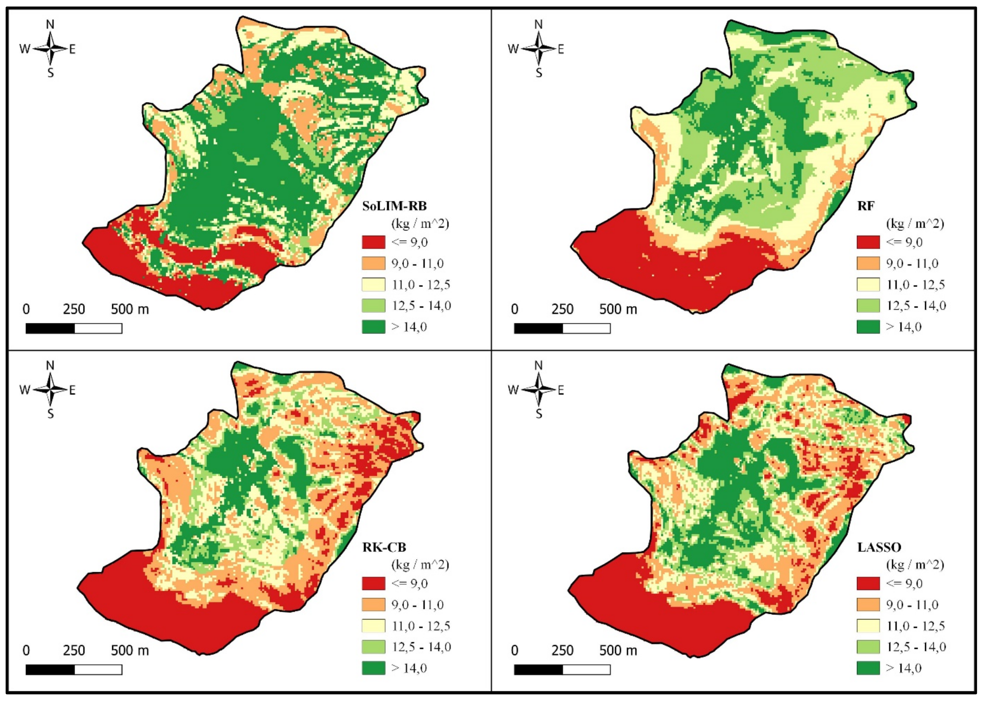
In the Vemvane catchment (Figure 8), the models that reflected the lowest error were the SoLIM-RB, RF, RK-CB, and LASSO models. The SoLIM-RB predicted a total SOC of 18.20 kt, the RF model predicted it to be 17.45 kt, the RK-CB predicted 15.59 kt, and the LASSO model predicted a total of 15.61 kt. However, it should be noted that even though the models predicted total SOC in the Vemvane catchment, all models had inaccurate results during the validation process.
4. Discussion
4.1. Relationship between SOC and Bulk Density
Higher values for depth of a profile and the SOC content will ultimately increase the total SOCs, whereas lower bulk density and higher rock fraction will decrease the total SOCs, as evident in studies from [14,39]. When discussing SOC content one can state that all the catchments can be considered carbon hotspots in a Southern African context. This is evident where it was found that only 4% of South African soils exceed 2% organic carbon [40]. Therefore, these soils have high SOCs considering the relatively shallow profiles encountered. On the other hand, due to the higher amount of SOC content the soils experience lower bulk densities. Research has reflected that an increase in SOC content causes a decrease in bulk density [37,39].
4.2. Covariate Importance
Recent research outlined the importance of vegetation indices for predicting SOCs [12,15], and the vertical distance from the valley bottom where sediment can accumulate [8]. However, covariate selection can be laborious to formalise into clear rules or mathematical equations because the knowledge is experiential and unsystematised [31]. In this study, the high MrRTF value for the Vemvane coupled with low EVI values (Table 4) created a problem for extrapolation. This could have been due to the difference in topography between the original, calibrated catchment (Tugela), and the Vemvane, where the original model was calibrated on the summit areas having small ridgetops and shallow profiles. This is evident in a study by [41], where they extrapolated a model to another area within the same region and found that a model performs best when there is a strong similarity between the calibrated area and the extrapolated area. Thus, models that are extrapolated from an area that is similar to the calibrated area, in their respective covariate values could perform well in the process.
4.3. Extrapolation Success
The analysis of extrapolated models (Figure 4) reflected that the RK-CB, LASSO, and UK models performed well during extrapolation except for the Vemvane catchments, where all the models performed undesirably. Throughout the catchments, the LASSO and UK models performed similarly with the LASSO performing slightly better regarding the NRMSE. The SoLIM models did not extrapolate well, with having substandard statistical performance as shown by the R2, NRMSE, and concordance (ρc).
When comparing [18]’s RK-CB’s results from the Tugela study (R2 = 0.61, NRMSE = 0.204, and ρc = 0.71) to the mean results of the Motete catchments (R2 = 0.61, NRMSE = 0.184, and ρc = 0.65), one can observe that the model performed similar during extrapolation, whereas the results from [18] in the Tugela for UK (R2 = 0.48, NRMSE = 0.235, and ρc = 0.61) and LASSO (R2 = 0.48, NRMSE = 0.236, and ρc = 0.59) yielded better mean results when extrapolated to the Motete catchments with UK (R2 = 0.66, NRMSE = 0.200, and ρc = 0.72) and LASSO (R2 = 0.67, NRMSE = 0.191, and ρc = 0.73). Therefore, in terms of consistency the RK-CB could be considered the most stable model to use for extrapolation. However, UK and LASSO can still be effective models to extrapolate.
In the case of the Vemvane, none of the models had satisfactory results, which could be due to certain relationships between SOCs, and covariates were not clearly defined than that of the calibrated area. This can influence the performance of a model by affecting the validity of coefficients [42]. However, in general the fuzzy membership models (SoLIM-RB and SoLIM-SB) and the tree model (RF) did not adapt well to the extrapolation, which could be due to the high variance of observed SOCs between and within the catchments. In contrast, the hybrid models (CB-RK and UK) and the linear regression model (LASSO) adapted well to the variation of SOCs between catchments and within.
There are three main factors that could influence the accuracy of extrapolated models. First, a model can have weak predictive capabilities when extrapolated can be a mismatch of the model structure and/or model coefficients [42]. In the case of this study, the more accurate predictions could be due to the effective use of the coefficients assigned to the model equations, where the model can adjust the predictions when encountering higher or lower values in the ancillary data prior to the extrapolation process. Another reason for the failure of extrapolated models could be if there is a lack of spatial correlation between the calibrated area and extrapolated area it can result in decreased predictive accuracy [16]. Last, prediction uncertainty was added because the SOCs was determined for the whole profile of a sampling site and not in predefined depths, it thus added uncertainty due to the depth varying among profiles from different sampling locations that result in a substantial difference between stock values. The majority of soil carbon studies are restricted to the upper 15 cm to 30 cm of soil due to the difficult nature of sampling and classification of the soil profiles [43].
4.4. Comparison of Maps and Trends
All four of the well performing M1 models (Figure 5) reflect to some extent the same trend, where higher SOCs is found in and around the valley bottom with a gentle slope. It is also where denser vegetative cover and the zone for accumulation can be found [15,39]. As with M1, the M2 catchment (Figure 7) also reflected that lower SOCs is mostly concentrated around the edge of the area, at higher vertical distance from the valley bottom, close to steep slopes. It was interesting to note that there were some areas with high SOCs values encounter at height, which were found to be seep wetlands that managed to flourish against a relatively steep slope. These wetlands are often located on top of mountains, and against steep slopes with colluvial soil, that is transported downslope by one-way water flow [44]. The EVI did manage to pick up these wetlands due to the dense vegetative cover in the form of normal short grass with hardly any bare patches. In the M3 catchment (Figure 7), there were also some seep wetlands encountered, where the LASSO (Figure 7a) and UK (Figure 7b) models managed to account for these areas. The RK-CB model (Figure 7c) managed to account to some extent the possibility of high SOCs values at increasing vertical distance, whereas the RF model (Figure 7d) struggled to accurately map the catchment. Although these models differ in the finer detail, they all managed to keep a trend for the SOCs distribution.
The Vemvane catchment (Figure 8) can be considered the ‘odd one out’ in this study, based on the poor results from extrapolation. The poor results could be due to the lack of similarity to the Tugela catchment, as [41] pointed out that similarity or areas can affect a model’s performance when extrapolated. The catchment overall had the lowest SOC content (4.17%) with relatively high rock fraction and shallow profiles, which resulted in the lowest mean SOCs of all. An added factor that could have contributed to the models’ results were that some of the profiles found at high vertical distance to the channel network had good depth. This was contradictory to the profiles encounter in the other catchments, which caused higher observed SOCs where the model predicted low. On the other hand, degradation differences of the Vemvane and Tugela can be ruled out as the cause for poor extrapolation results, because [45] found that both the Vemvane and Tugela experiences the same level of degradation.
The Maloti-Drakensberg region has proved to be a carbon hotspot worthy of further research and stakeholder involvement. In terms of carbon credits there is a good opportunity for mines to become involved in rehabilitating the degraded wetlands. It could not only be a financial gain for them, but also a win for the alpine wetlands and the ecosystem services they offer. However, the right model should be selected when mapping the alpine region, as evident by the difference of predicted total SOC each mapping method yields. For instance, the difference in the M1 catchment between the model with the highest prediction (SoLIM-RB) and lowest (SoLIM-SB) is 7.90 kt, whereas the M2 catchment’s difference is 3.88 kt between the SoLIM-RB (highest) and RF (lowest). Similarly, M3 had a difference of 5.56 kt difference the SoLIM-RB (highest) and RF (lowest) models. These differences can make a significant difference when calculating carbon credits or sequestration capabilities.
5. Conclusions
In regard to finding a model that can be used to map the greater Maloti-Drakensberg region, the Vemvane catchment presented a problem for extrapolating the most successful model (RK-CB), even though the Motete models exceeded expectations. Thus, the complexity of the Maloti-Drakensberg terrain can create uncertainty, especially when the terrain and vegetation attributes differ among catchments. This can cause SOCs distribution to follow different trends depending on the state of a catchment. Therefore, if the one would consider mapping a large area by training models with a single catchment, that catchment should be a good representative of the general trend observed in the region. With this study, one can learn that close proximity does not equal good similarity.
Author Contributions
Conceptualization, J.K. and J.v.T.; fieldwork and data acquisition, J.K. and J.v.T.; laboratory analysis, modelling and data interpretation, J.K.; writing—original draft preparation, J.K.; writing—review and editing, J.v.T.; supervision, J.v.T.; project administration, J.v.T. All authors have read and agreed to the published version of the manuscript.
Funding
The authors would like to acknowledge incentive funding from the National Research Foundation (NRF) to J.v.T. as well as funding from the Afromontane Research Unit (ARU) of the University of the Free State (UFS) to J.K.
Data Availability Statement
Data available from the first order on request.
Acknowledgments
We would first like to acknowledge the Afromontane research unit (ARU) for providing a bursary to J.K. We also thank the Witsieshoek Mountain Lodge for accommodating the team members during the visits. We thank the Royal Natal National Park for allowing research in the protected area. We thank Frances Kotzé, Cowan McLean, Matthew Mamera, and Alec Edwards for the assistance during filed visits. We thank Boingotlo Tshabang for assistance in analyzing the soil samples gathered.
Conflicts of Interest
The authors declare no conflict of interest. The funders had no role in the design of the study; in the collection, analyses, or interpretation of data; in the writing of the manuscript; or in the decision to publish the results.
References
- Ellili, Y.; Walter, C.; Michot, D.; Pichelin, P.; Lemercier, B. Mapping soil organic carbon stock change by soil monitoring and digital soil mapping at the landscape scale. Geoderma 2019, 351, 1–8. [Google Scholar] [CrossRef]
- Lorenz, K.; Lal, R. Soil Organic Carbon: An Appropriate Indicator to Monitor Trends of Land and Soil Degradation within the SDG Framework; Umweltbundesamt: Dessau-Roßlau, Germany, 2016; pp. 14–22. [Google Scholar]
- Schulze, R.E.; Schütte, S. Mapping soil organic carbon at a terrain unit resolution across South Africa. Geoderma 2020, 373, 114447. [Google Scholar] [CrossRef]
- Wang, M.; Yang, W.; Wu, N.; Wu, Y.; Lafleur, P.; Lu, T. Patterns and drivers of soil carbon stock in southern China’s grasslands. Agric. For. Meteorol. 2019, 276, 107634. [Google Scholar] [CrossRef]
- Muñoz, M.A.; Faz, A.; Zornoza, R. Carbon stocks and dynamics in grazing highlands from the Andean Plateau. Catena 2013, 104, 136–143. [Google Scholar] [CrossRef]
- Conant, R.T. Challenges and Opportunities for Carbon Sequestration in Grassland Systems: A Technical Report on Grassland Management and Climate Change Mitigation. In Integrated Crop Management; FAO Publishing: Rome, Italy, 2010; Volume 9, pp. 5–22. [Google Scholar]
- Otte, J.; Pica-Ciamarra, U.; Morzaria, S. A comparative overview of the livestock-environment interactions in Asia and Sub-Saharan Africa. Front. Vet. Sci. 2019, 6, 37. [Google Scholar] [CrossRef] [Green Version]
- van Zijl, G.M.; Bouwer, D.; van Tol, J.J.; Le Roux, P.A.L. Functional digital soil mapping: A case study from Namarroi, Mozambique. Geoderma 2014, 219, 155–161. [Google Scholar] [CrossRef]
- McBratney, A.B.; Mendonça Santos, M.L.; Minasny, B. On digital soil mapping. Geoderma 2003, 117, 3–52. [Google Scholar] [CrossRef]
- Adhikari, K.; Hartemink, A.E.; Minasny, B.; Bou Kheir, R.; Greve, M.B.; Greve, M.H. Digital mapping of soil organic carbon contents and stocks in Denmark. PLoS ONE 2014, 9, 105519. [Google Scholar] [CrossRef]
- Simón, N.; Montes, F.; Díaz-Pinés, E.; Benavides, R.; Roig, S.; Rubio, A. Spatial distribution of the soil organic carbon pool in a Holm oak dehesa in Spain. Plant Soil 2013, 366, 537–549. [Google Scholar] [CrossRef] [Green Version]
- Yang, R.M.; Zhang, G.L.; Liu, F.; Lu, Y.Y.; Yang, F.; Yang, F.; Yang, M.; Zhao, Y.G.; Li, D.C. Comparison of boosted regression tree and random forest models for mapping topsoil organic carbon concentration in an alpine ecosystem. Ecol. Indic. 2016, 60, 870–878. [Google Scholar] [CrossRef]
- Gomes, L.C.; Faria, R.M.; de Souza, E.; Veloso, G.V.; Schaefer, C.E.G.; Fernandes Filho, E.I. Modeling and mapping soil organic carbon stocks in Brazil. Geoderma 2019, 340, 337–350. [Google Scholar] [CrossRef]
- Seboko, K.R.; Kotze, E.; van Tol, J.; van Zijl, G. Characterization of Soil Carbon Stocks in the City of Johannesburg. Land 2021, 10, 83. [Google Scholar] [CrossRef]
- Matinfar, H.R.; Maghsodi, Z.; Mousavi, S.R.; Rahmani, A. Evaluation and Prediction of Topsoil organic carbon using Machine learning and hybrid models at a Field-scale. Catena 2021, 202, 105258. [Google Scholar] [CrossRef]
- Grinand, C.; Arrouays, D.; Laroche, B.; Martin, M.P. Extrapolating regional soil landscapes from an existing soil map: Sampling intensity, validation procedures, and integration of spatial context. Geoderma 2008, 143, 180–190. [Google Scholar] [CrossRef]
- Du, L.; McCarty, G.W.; Li, X.; Rabenhorst, M.C.; Wang, Q.; Lee, S.; Hinson, A.L.; Zou, Z. Spatial extrapolation of topographic models for mapping soil organic carbon using local samples. Geoderma 2021, 404, 115290. [Google Scholar] [CrossRef]
- Kotzé, J. Quantifying Soil Carbon Stocks in Alpine Areas of the Maloti-Drakensberg Mountains Using Digital Soil Mapping Approaches. Master’s Thesis, University of the Free State, Bloemfontein, South Africa, 2022; pp. 43–74. [Google Scholar]
- Finch, J.M.; Hill, T.R.; Meadows, M.E.; Lodder, J.; Bodmann, L. Fire and montane vegetation dynamics through successive phases of human occupation in the northern Drakensberg, South Africa. Quat. Int. 2022, 611, 66–76. [Google Scholar] [CrossRef]
- Mokotjomela, T.; Schwaibold, U.; Pillay, N. Does the ice rat Otomys sloggetti robertsi contribute to habitat change in Lesotho? Acta Oecol. 2009, 35, 437–443. [Google Scholar] [CrossRef]
- Cole, M.J.; Bailey, R.M.; Cullis, J.D.; New, M.G. Spatial inequality in water access and water use in South Africa. Water Policy 2018, 20, 37–52. [Google Scholar] [CrossRef]
- Carbutt, C. The Drakensberg Mountain Centre: A necessary revision of southern Africa’s high-elevation centre of plant endemism. S. Afr. J. Bot. 2019, 124, 508–529. [Google Scholar] [CrossRef]
- Zhu, A.X.; Burt, J.E.; Du, F. SoLIM Solutions Help Manual: For SoLIM Solution 2016. 2015. Available online: https://lreis2415.github.io/SoLIMSolutions/software.html (accessed on 28 January 2022).
- Zhu, A.X.; Hudson, B.; Burt, J.; Lubich, K.; Simonson, D. Soil mapping using GIS, expert knowledge, and fuzzy logic. Soil Sci. Soc. Am. J. 2001, 65, 1463–1472. [Google Scholar] [CrossRef] [Green Version]
- Malone, B.P.; Minasny, B.; McBratney, A.B. Using R for Digital Soil Mapping, 1st ed.; Springer International Publishing: Cham, Switzerland, 2017; pp. 117–149. [Google Scholar]
- Nussbaum, M.; Spiess, K.; Baltensweiler, A.; Grob, U.; Keller, A.; Greiner, L.; Schaepman, M.E.; Papritz, A. Evaluation of digital soil mapping approaches with large sets of environmental covariates. Soil 2018, 4, 1–22. [Google Scholar] [CrossRef] [Green Version]
- Kerr, D.D.; Ochsner, T.E. Soil organic carbon more strongly related to soil moisture than soil temperature in temperate grasslands. Soil Sci. Soc. Am. J. 2020, 84, 587–596. [Google Scholar] [CrossRef] [Green Version]
- Lamichhane, S.; Kumar, L.; Wilson, B. Digital soil mapping algorithms and covariates for soil organic carbon mapping and their implications: A review. Geoderma 2019, 352, 395–413. [Google Scholar] [CrossRef]
- Minasny, B.; McBratney, A.B. A conditioned Latin hypercube method for sampling in the presence of ancillary information. Comput. Geosci. 2006, 32, 1378–1388. [Google Scholar] [CrossRef]
- Yang, L.; Li, X.; Shi, J.; Shen, F.; Qi, F.; Gao, B.; Chen, Z.; Zhu, A.X.; Zhou, C. Evaluation of conditioned Latin hypercube sampling for soil mapping based on a machine learning method. Geoderma 2020, 369, 114337. [Google Scholar] [CrossRef]
- Liang, P.; Qin, C.Z.; Zhu, A.X.; Hou, Z.W.; Fan, N.Q.; Wang, Y.J. A case-based method of selecting covariates for digital soil mapping. J. Integr. Agric. 2020, 19, 2127–2136. [Google Scholar] [CrossRef]
- Clifford, D.; Payne, J.E.; Pringle, M.J.; Searle, R.; Butler, N. Pragmatic soil survey design using flexible Latin hypercube sampling. Comput. Geosci. 2014, 67, 62–68. [Google Scholar] [CrossRef]
- Soil Classification Working Group. Soil classification: A Natural and Anthropogenic System for South Africa; ARC-Institute for Soil, Climate and Water: Pretoria, South Africa, 2018. [Google Scholar]
- Razakamanarivo, R.H.; Grinand, C.; Razafindrakoto, M.A.; Bernoux, M.; Albrecht, A. Mapping organic carbon stocks in eucalyptus plantations of the central highlands of Madagascar: A multiple regression approach. Geoderma 2011, 162, 335–346. [Google Scholar] [CrossRef]
- Jabro, J.D.; Stevens, W.B.; Iversen, W.M. Comparing two methods for measuring soil bulk density and moisture content. Open J. Soil Sci. 2020, 10, 233–243. [Google Scholar] [CrossRef]
- Ramifehiarivo, N.; Brossard, M.; Grinand, C.; Andriamananjara, A.; Razafimbelo, T.; Rasolohery, A.; Razafimahatratra, H.; Seyler, F.; Ranaivoson, N.; Rabenarivo, M.; et al. Mapping soil organic carbon on a national scale: Towards an improved and updated map of Madagascar. Geoderma Reg. 2017, 9, 29–38. [Google Scholar] [CrossRef]
- Zhang, Y.; Ai, J.; Sun, Q.; Li, Z.; Hou, L.; Song, L.; Tang, G.; Li, L.; Shao, G. Soil organic carbon and total nitrogen stocks as affected by vegetation types and altitude across the mountainous regions in the Yunnan Province, south-western China. Catena 2021, 196, 104872. [Google Scholar] [CrossRef]
- Salehi Rizi, F.; Granitzer, M. Properties of vector embeddings in social networks. Algorithms 2017, 10, 109. [Google Scholar] [CrossRef] [Green Version]
- Dorji, T.; Odeh, I.O.; Field, D.J.; Baillie, I.C. Digital soil mapping of soil organic carbon stocks under different land use and land cover types in montane ecosystems, Eastern Himalayas. For. Ecol. Manag. 2014, 318, 91–102. [Google Scholar] [CrossRef]
- du Preez, C.C.; van Huyssteen, C.W.; Mnkeni, P.N. Land use and soil organic matter in South Africa 2: A review on the influence of arable crop production. S. Afr. J. Sci. 2011, 107, 1–8. [Google Scholar] [CrossRef] [Green Version]
- Malone, B.P.; Jha, S.K.; Minasny, B.; McBratney, A.B. Comparing regression-based digital soil mapping and multiple-point geostatistics for the spatial extrapolation of soil data. Geoderma 2016, 262, 243–253. [Google Scholar] [CrossRef]
- Angelini, M.E.; Kempen, B.; Heuvelink, G.B.M.; Temme, A.J.; Ransom, M.D. Extrapolation of a structural equation model for digital soil mapping. Geoderma 2020, 367, 114226. [Google Scholar] [CrossRef]
- Don, A.; Schumacher, J.; Scherer-Lorenzen, M.; Scholten, T.; Schulze, E.D. Spatial and vertical variation of soil carbon at two grassland sites—Implications for measuring soil carbon stocks. Geoderma 2007, 141, 272–282. [Google Scholar] [CrossRef]
- Job, N.; Mbona, N.; Dayaram, A.; Kotze, D.C. Guidelines for Mapping Wetlands in South Africa, 1st ed.; SANBI Biodiversity Series 28; SANBI Biodiversity: Pretoria, South Africa, 2018; pp. 28–40. [Google Scholar]
- Mathinya, N.V.; Clark, V.R.; van Tol, J.J.; Franke, A.C. Resilience and Sustainability of the Maloti-Drakensberg Mountain System: A Case Study on the Upper uThukela Catchment. In Human-Nature Interactions: Exploring Nature’s Values Across Landscapes; Misiune, I., Depellegrin, D., Egarter, V.L., Eds.; Springer International Publishing: Cham, Switzerland, 2022; pp. 155–167. [Google Scholar]
Figure 1.
Tugela, Vemvane, and Motete headwater catchments. The Motete catchments are in Lesotho, whereas the Vemvane catchment in within the Free State Province in South Africa, next to the Tugela catchment.
Figure 1.
Tugela, Vemvane, and Motete headwater catchments. The Motete catchments are in Lesotho, whereas the Vemvane catchment in within the Free State Province in South Africa, next to the Tugela catchment.
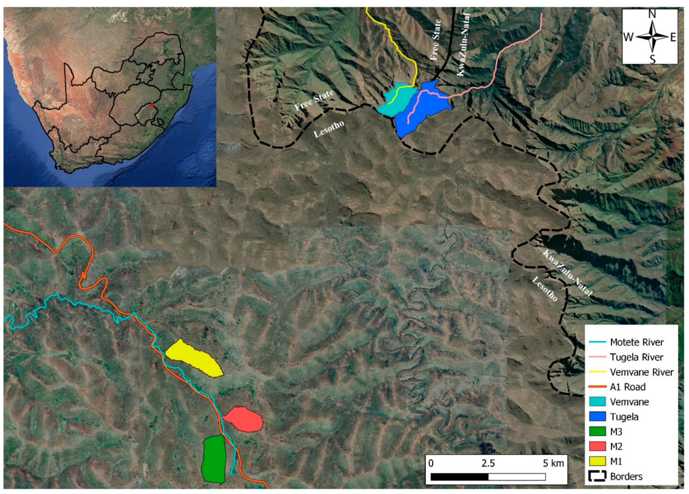
Figure 2.
The locations from where samples were collected. (a) Tugela catchment with its calibration and validation samples, (b) the Vemvane catchment with only validation samples, and (c) the Motete catchments with validation samples from each of the three.
Figure 2.
The locations from where samples were collected. (a) Tugela catchment with its calibration and validation samples, (b) the Vemvane catchment with only validation samples, and (c) the Motete catchments with validation samples from each of the three.

Figure 3.
The relative covariate importance plot gained from the Random Forest (RF) model. The importance is assigned based on the percentage increase in MSE that would occur from removing each covariate.
Figure 3.
The relative covariate importance plot gained from the Random Forest (RF) model. The importance is assigned based on the percentage increase in MSE that would occur from removing each covariate.
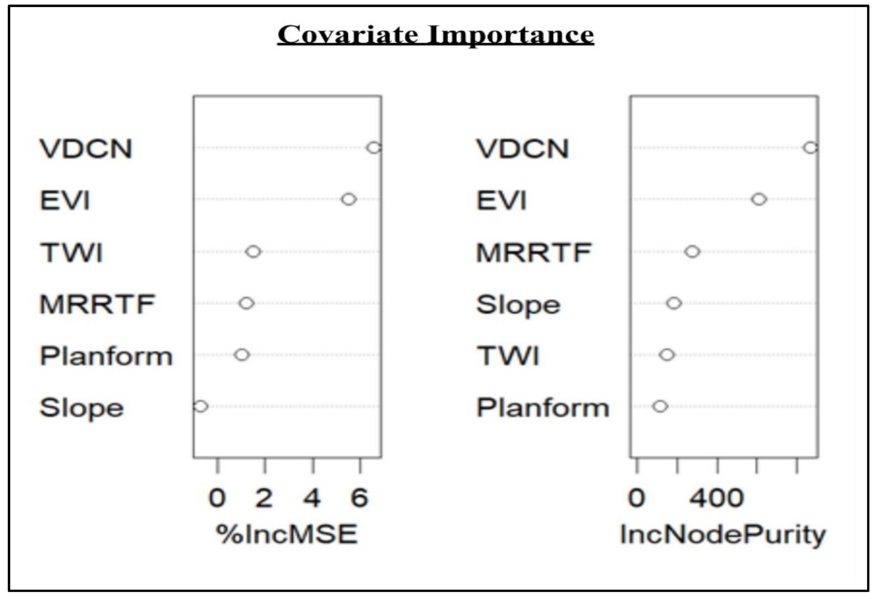
Figure 4.
Linear regressions of inferred and observed SOCs for all models in M1 (a), M2 (b), M3 (c), and Vemvane (d). The statistical indicators used were R2, normalized root mean squared error (NRMSE), and the concordance coefficient (ρc). The dotted line reflects the 45° line that provides a 1:1 ratio for predicted and observed values, whereas the red line illustrates the regression line.
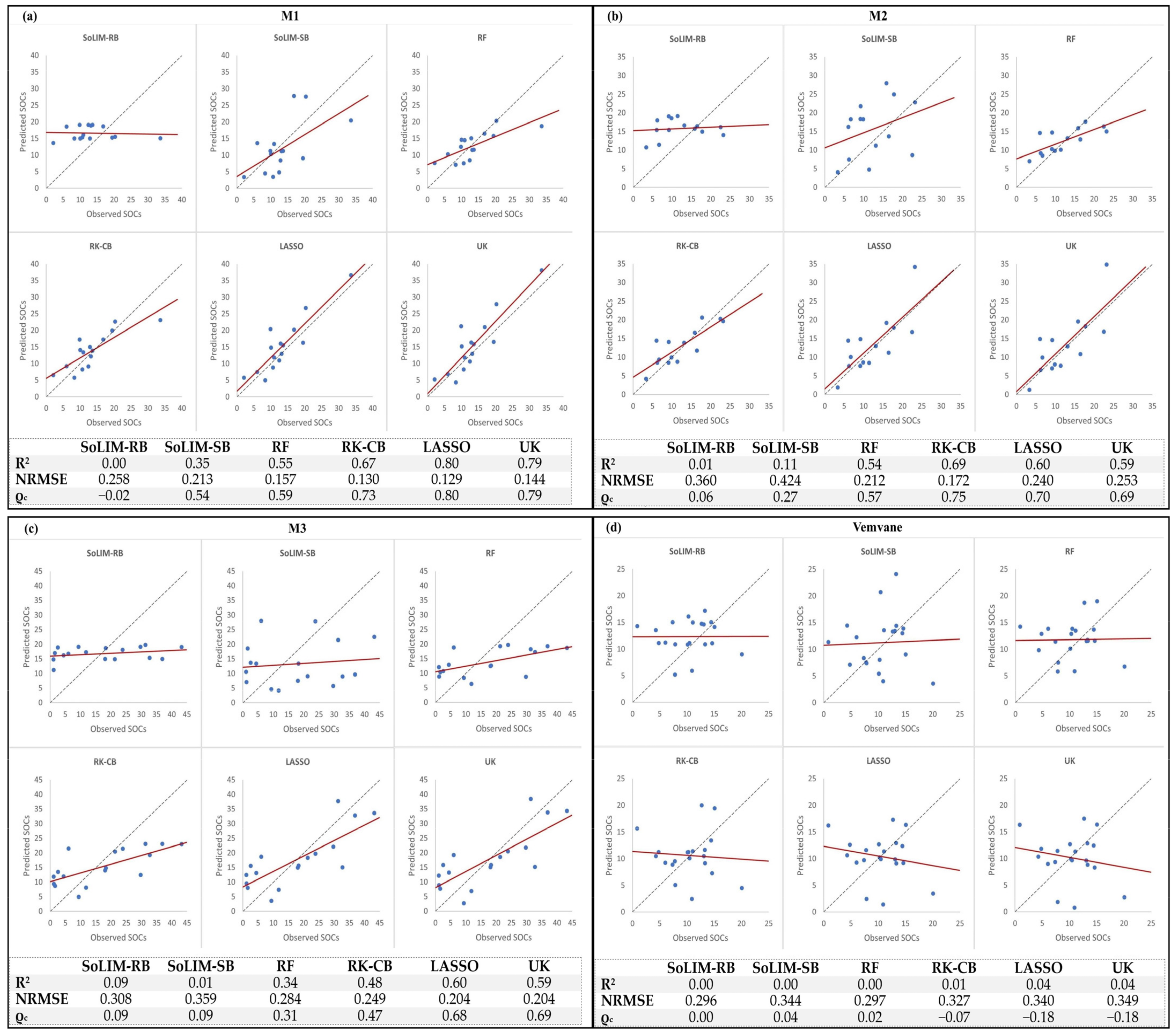
Figure 5.
A comparison between the M1 catchment’s (a) LASSO, (b) RK-CB, (c) RF, and (d) UK, in order of their performance in regard to error (NRMSE).
Figure 5.
A comparison between the M1 catchment’s (a) LASSO, (b) RK-CB, (c) RF, and (d) UK, in order of their performance in regard to error (NRMSE).

Figure 6.
A comparison between the M2 catchment’s (a) RK-CB, (b) RF, (c) LASSO, and (d) UK, in order of their performance in regard to error (NRMSE).
Figure 6.
A comparison between the M2 catchment’s (a) RK-CB, (b) RF, (c) LASSO, and (d) UK, in order of their performance in regard to error (NRMSE).
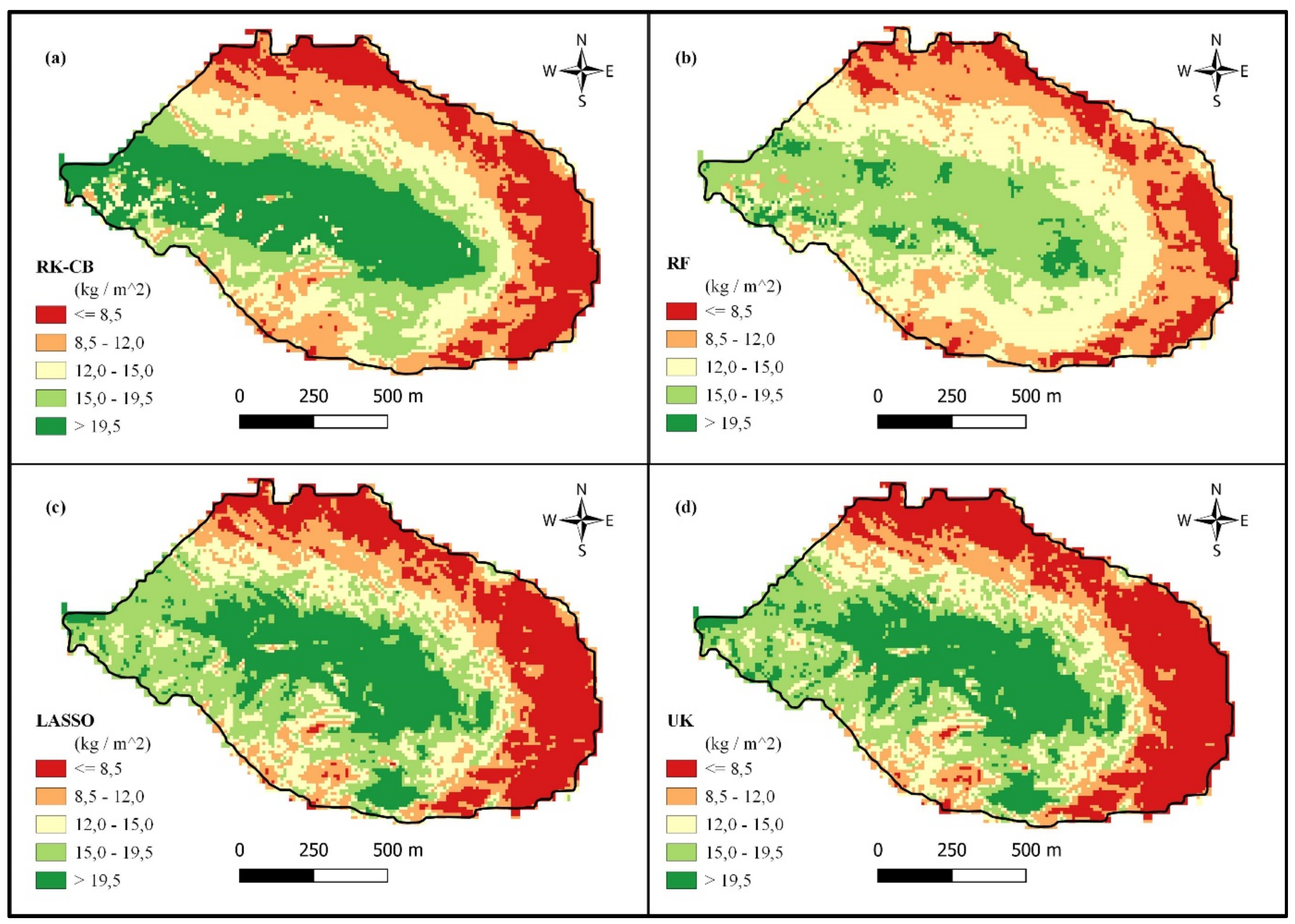
Figure 7.
A comparison between the M3 catchment’s (a) LASSO, (b) UK, (c) RK-CB, and (d) RF, in order of their performance in regard to error (NRMSE).
Figure 7.
A comparison between the M3 catchment’s (a) LASSO, (b) UK, (c) RK-CB, and (d) RF, in order of their performance in regard to error (NRMSE).
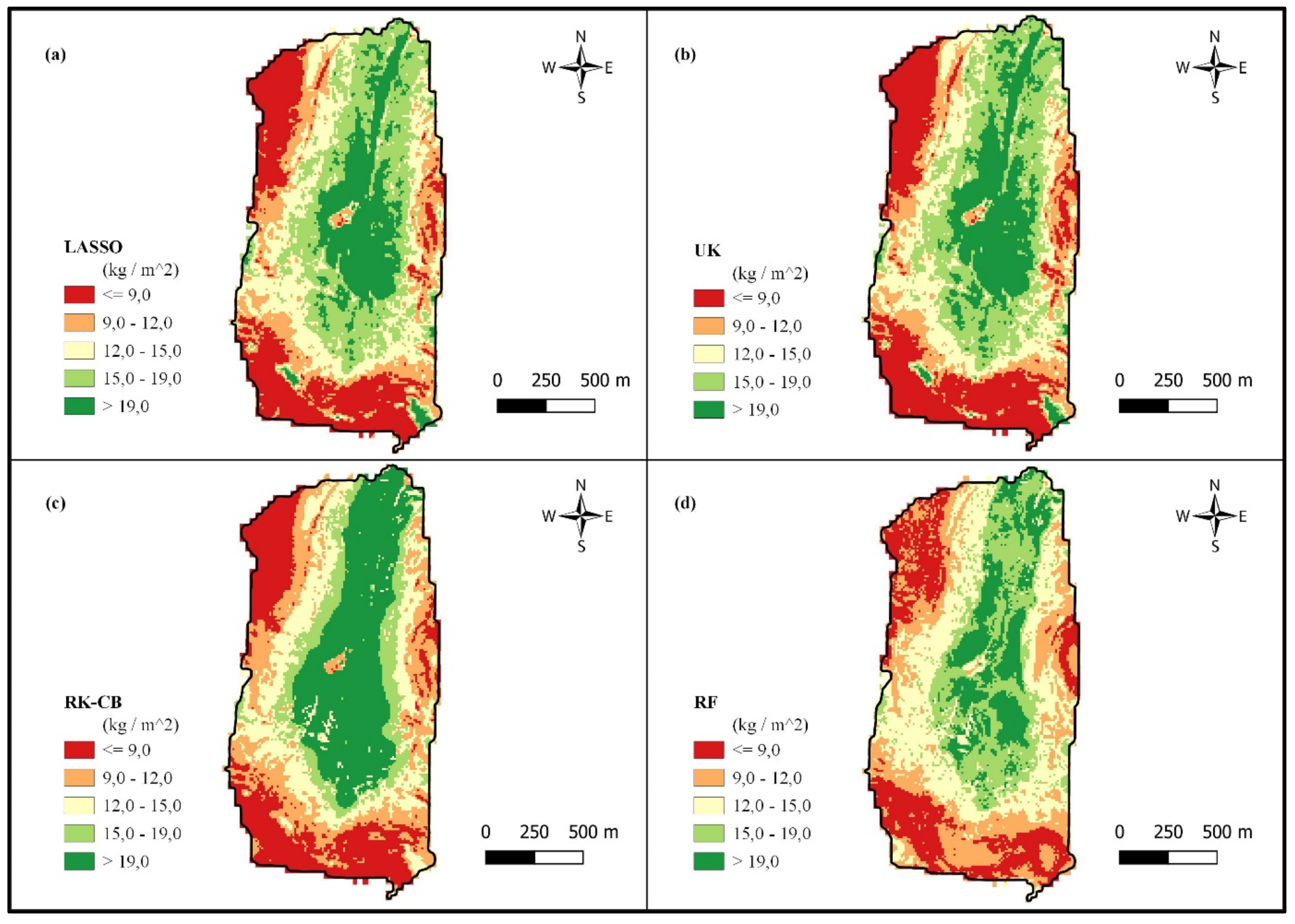
Figure 8.
A comparison between the Vemvane catchment’s SoLIM-RB, RF, RK-CB, and LASSO, in order of their performance in regard to error (NRMSE).
Figure 8.
A comparison between the Vemvane catchment’s SoLIM-RB, RF, RK-CB, and LASSO, in order of their performance in regard to error (NRMSE).

Table 1.
Fuzzy membership rules created based on expert knowledge of the landscape in order to create the SoLIM-RB model for the Tugela catchment [18].
Table 1.
Fuzzy membership rules created based on expert knowledge of the landscape in order to create the SoLIM-RB model for the Tugela catchment [18].
| Soil Association | Soil-Landscape Rules | ||||
|---|---|---|---|---|---|
| Vertical Distance to Channel Network (VDCN) | Slope Percentage | Topographic Wetness Index (TWI) | Multiresolution Index Valley Bottom Flatness (MrVBF) | Normalized Difference Vegetation Index (NDVI) | |
| Organic | <7 m | <8% | >12 | >2 | >0.16 |
| Shallow Humic (Hs) | <35 m | 8–13% | 7–12 | 0.3–2 | >0.16 |
| Deep Humic (Hd) | 35–60 m | 13–18% | 7–12 | 0.01–1 | >0.16 |
| Deep Orthic (Od) | 35–80 m | 18–25% | <7 | 0.01–1 | <0.16 |
| Shallow Orthic (Os) | >60 m | >25% | <7 | <0.01 | <0.16 |
Table 2.
Summary of the terrain and vegetation covariates created from the DEM and Sentinel 2 used in the study.
Table 2.
Summary of the terrain and vegetation covariates created from the DEM and Sentinel 2 used in the study.
| Covariates | Type | Description | Required |
|---|---|---|---|
| Enhanced vegetation index (EVI) | Vegetation | Vegetation index with canopy background and atmospheric corrections. | Multispectral scanner |
| Multiresolution index of ridge top flatness (MrRTF) | Morphometry | Identify higher areas of a landscape and characterize its flatness. | DEM |
| Planform curvature | Morphometry | Characterize flow as either convergence or divergence. | DEM |
| TWI | Hydrology | Quantifies the influence of topography on hydrological processes. | Slope and catchment area |
| Slope | Morphometry | The measurement of steepness or the degree of inclination. | DEM |
| VDCN | Hydrology | An interpolated value of a location for the height above a river network. | DEM and channel network |
Table 3.
Summary of all the catchments’ SOCs, SOC content, soil bulk density, and the rock fraction (mean ± standard deviation).
Table 3.
Summary of all the catchments’ SOCs, SOC content, soil bulk density, and the rock fraction (mean ± standard deviation).
| Number of Samples (n) | Depth (cm) | Bulk Density (g cm−3) | Rock Fraction | SOC Content (%) | SOCs (kg m−2) | |
|---|---|---|---|---|---|---|
| Tugela | 90 | 25 ± 13 | 0.96 ± 0.19 | 0.11 ± 0.06 | 6.26 ± 2.09 | 12.66 ± 7.02 |
| Vemvane | 20 | 28 ± 14 | 0.89 ± 0.09 | 0.10 ± 0.04 | 4.17 ± 2.03 | 10.43 ± 4.48 |
| M1 | 15 | 31 ± 16 | 0.85 ± 0.10 | 0.08 ± 0.03 | 7.90 ± 4.31 | 13.37 ± 7.33 |
| M2 | 14 | 34 ± 21 | 0.88 ± 0.14 | 0.08 ± 0.03 | 5.75 ± 2.87 | 12.23 ± 6.19 |
| M3 | 17 | 35 ± 27 | 0.87 ± 0.08 | 0.11 ± 0.03 | 6.58 ± 2.75 | 17.29 ± 13.88 |
Table 4.
Summary of all the catchments’ covariate values in terms of their minimum, maximum, mean, standard deviation, kurtosis, and skewness.
Table 4.
Summary of all the catchments’ covariate values in terms of their minimum, maximum, mean, standard deviation, kurtosis, and skewness.
| Covariates | Catchments | |||||
|---|---|---|---|---|---|---|
| Tugela | Vemvane | M1 | M2 | M3 | ||
| Planform | Min ± Max Mean ± SD Kurtosis Skewness | −0.002 ± 0.004 0.000 ± 0.001 1.50 0.80 | −0.002 ± 0.003 0.000 ± 0.001 1.36 0.60 | −0.002 ± 0.003 0.000 ± 0.001 0.85 0.40 | −0.002 ± 0.002 0.000 ± 0.001 0.75 0.65 | −0.001 ± 0.003 0.000 ± 0.001 0.56 0.82 |
| EVI | Min ± Max Mean ± SD Kurtosis Skewness | 0.02 ± 0.27 0.14 ± 0.03 0.42 0.52 | 0.04 ± 0.27 0.13 ± 0.03 0.91 0.67 | 0.07 ± 0.62 0.18 ± 0.05 15.60 2.73 | 0.04 ± 0.58 0.21 ± 0.08 2.25 1.53 | 0.06 ± 0.60 0.20 ± 0.07 5.62 2.19 |
| MrRTF | Min ± Max Mean ± SD Kurtosis Skewness | 0.00 ± 1.90 0.10 ± 0.22 20.50 4.11 | 0.00 ± 2.59 0.22 ± 0.36 9.08 2.79 | 0.00 ± 2.68 0.12 ± 0.32 19.00 4.10 | 0.00 ± 3.08 0.19 ± 0.38 17.30 3.89 | 0.00 ± 2.85 0.14 ± 0.32 19.40 4.04 |
| TWI | Min ± Max Mean ± SD Kurtosis Skewness | 4.24 ± 16.55 7.32 ± 1.81 4.31 1.85 | 4.27 ± 14.38 7.38 ± 1.49 1.27 1.09 | 4.79 ± 12.99 7.23 ± 1.41 2.46 1.56 | 5.32 ± 12.77 7.54 ± 1.37 0.81 1.11 | 5.10 ± 13.50 7.37 ± 1.43 2.39 1.49 |
| Slope | Min ± Max Mean ± SD Kurtosis Skewness | 0.5 ± 52.9 17.3 ± 8.4 0.16 0.53 | 1.5 ± 60.1 13.8 ± 9.2 1.66 1.28 | 1.9 ± 52.9 18.4 ± 7.7 −0.45 0.47 | 2.0 ± 28.7 13.3 ± 4.5 0.03 0.38 | 1.7 ± 35.4 15.6 ± 6.7 −0.57 0.28 |
| VDCN | Min ± Max Mean ± SD Kurtosis Skewness | 0.1 ± 133.6 33.8 ± 30.1 −0.003 0.93 | 0.3 ± 133.7 28.3 ± 31.3 1.27 1.51 | 0.3 ± 110.3 37.6 ± 29.5 −0.93 0.48 | 0.3 ± 103.0 35.9 ± 26.7 −0.96 0.40 | 0.3 ± 116.6 33.9 ± 28.5 −0.24 0.83 |
Disclaimer/Publisher’s Note: The statements, opinions and data contained in all publications are solely those of the individual author(s) and contributor(s) and not of MDPI and/or the editor(s). MDPI and/or the editor(s) disclaim responsibility for any injury to people or property resulting from any ideas, methods, instructions or products referred to in the content. |
© 2023 by the authors. Licensee MDPI, Basel, Switzerland. This article is an open access article distributed under the terms and conditions of the Creative Commons Attribution (CC BY) license (https://creativecommons.org/licenses/by/4.0/).
Share and Cite
MDPI and ACS Style
Kotzé, J.; van Tol, J. Extrapolation of Digital Soil Mapping Approaches for Soil Organic Carbon Stock Predictions in an Afromontane Environment. Land 2023, 12, 520. https://doi.org/10.3390/land12030520
AMA Style
Kotzé J, van Tol J. Extrapolation of Digital Soil Mapping Approaches for Soil Organic Carbon Stock Predictions in an Afromontane Environment. Land. 2023; 12(3):520. https://doi.org/10.3390/land12030520
Chicago/Turabian StyleKotzé, Jaco, and Johan van Tol. 2023. "Extrapolation of Digital Soil Mapping Approaches for Soil Organic Carbon Stock Predictions in an Afromontane Environment" Land 12, no. 3: 520. https://doi.org/10.3390/land12030520
Note that from the first issue of 2016, this journal uses article numbers instead of page numbers. See further details here.