
Investigating Near-Surface Hydrologic Connectivity in a Grass-Covered Inter-Row Area of a Hillslope Vineyard Using Field Monitoring and Numerical Simulations

 , , , , , and
Abstract
:
1. Introduction
2. Materials and Methods
2.1. Site Description
2.2. Soil Data
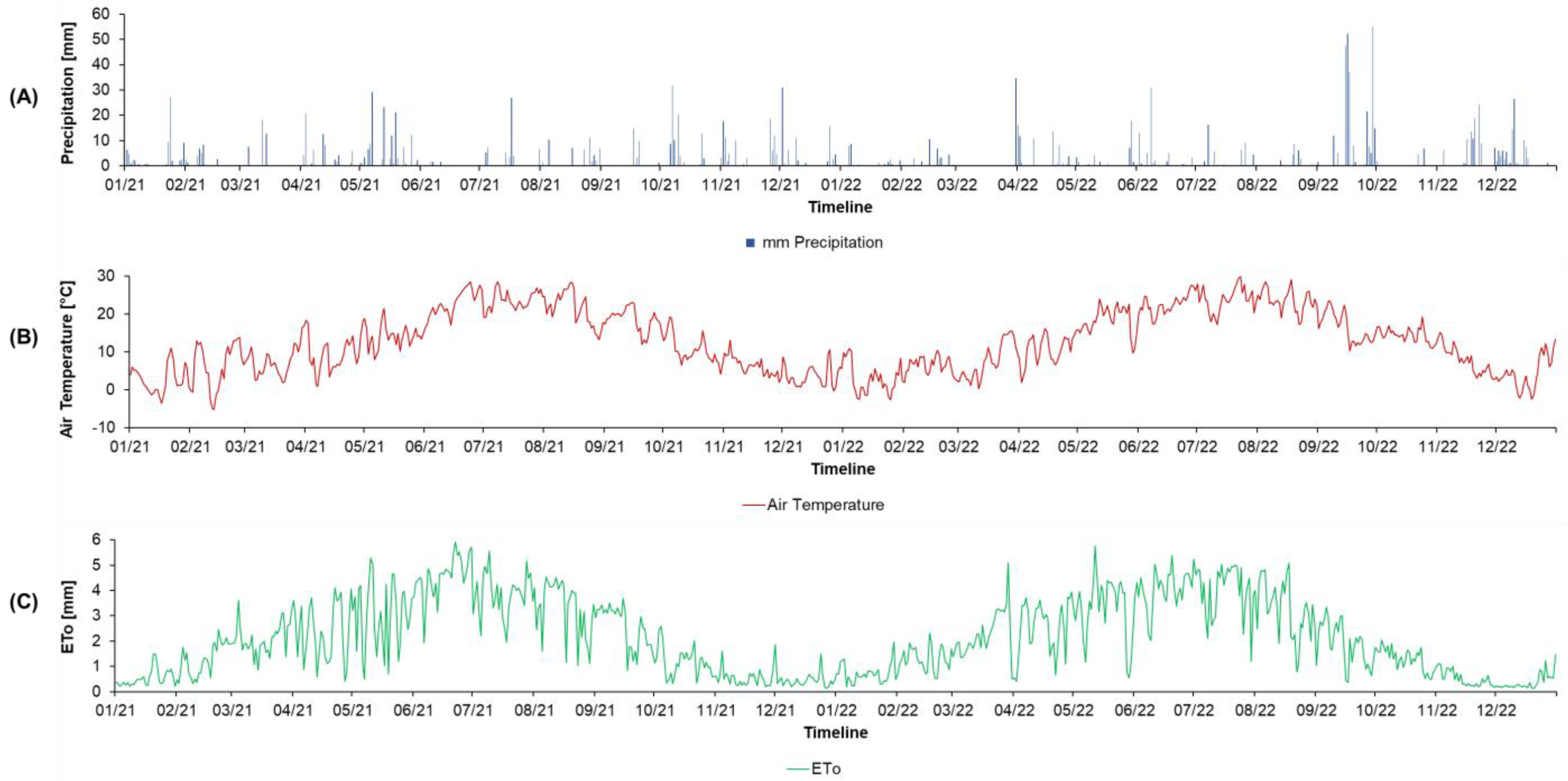
2.3. Meterorological Data
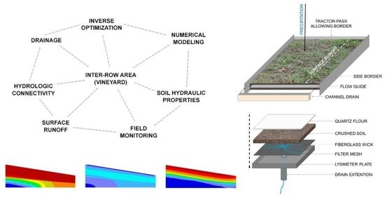
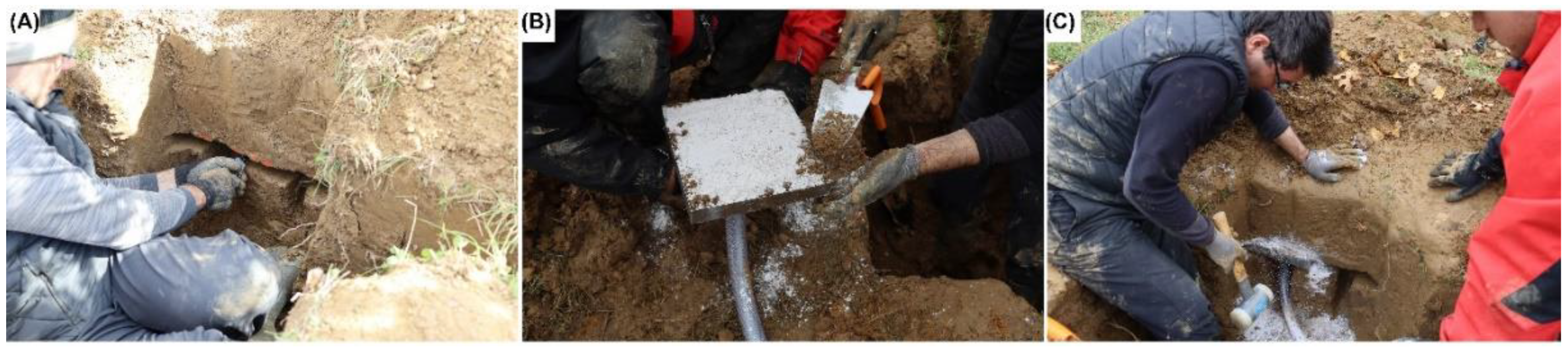
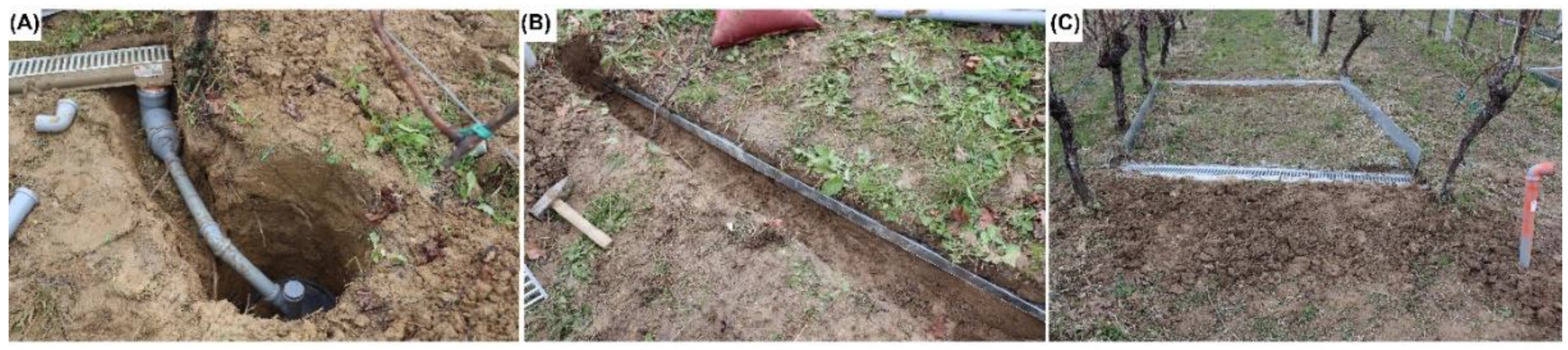
2.4. Field Monitoring of Soil Water Fluxes
2.5. Numerical Modeling
- Initial one-dimensional modeling based on laboratory determined SHPs, meteorological data and grass cover measurements;
- Inverse one-dimensional modeling based on lysimeter outflow to optimize hydraulic conductivity and to additionally evaluate the model-based surface runoff data;
- Two-dimensional modeling with the optimized parameters to investigate soil moisture in critical seasonal moments.
2.6. Statistical Analysis
3. Results
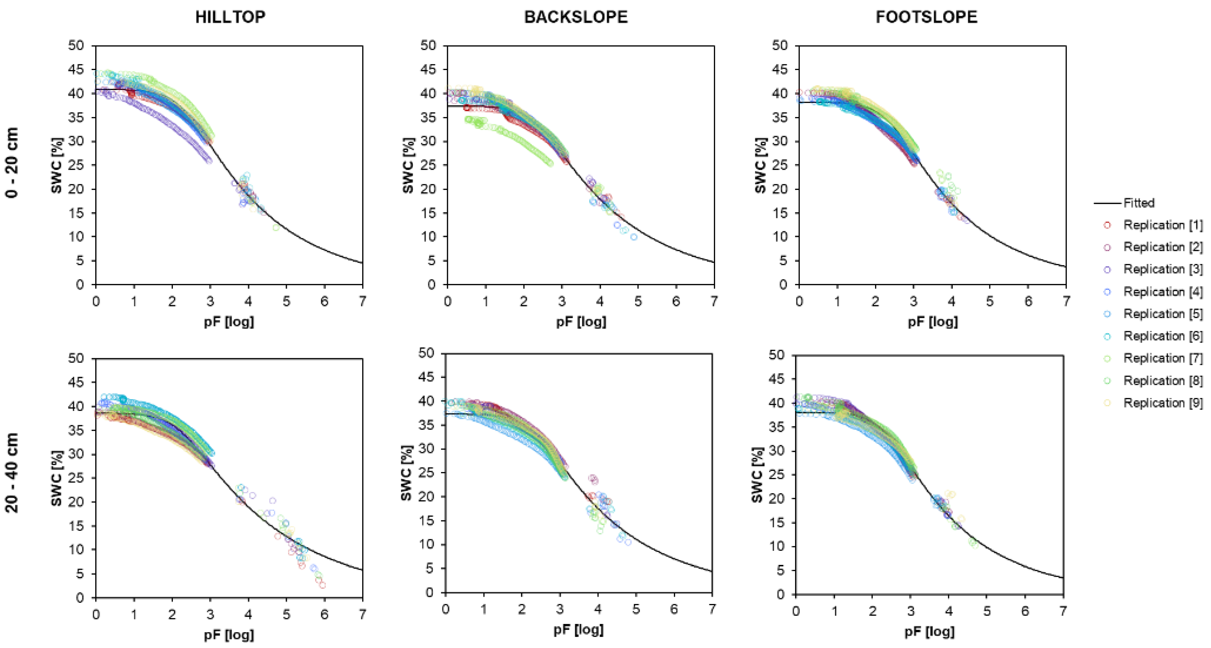
3.1. Soil Data
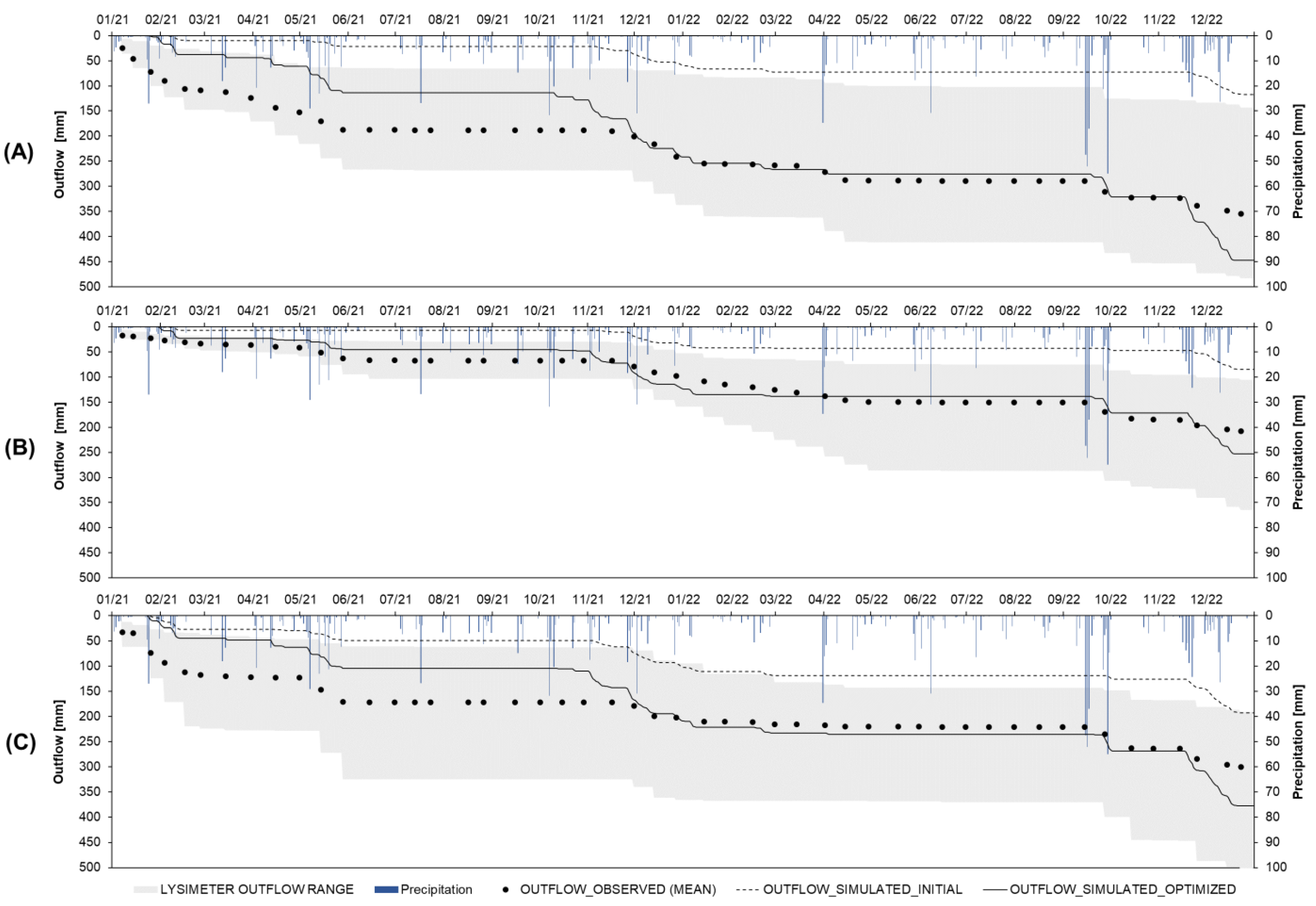
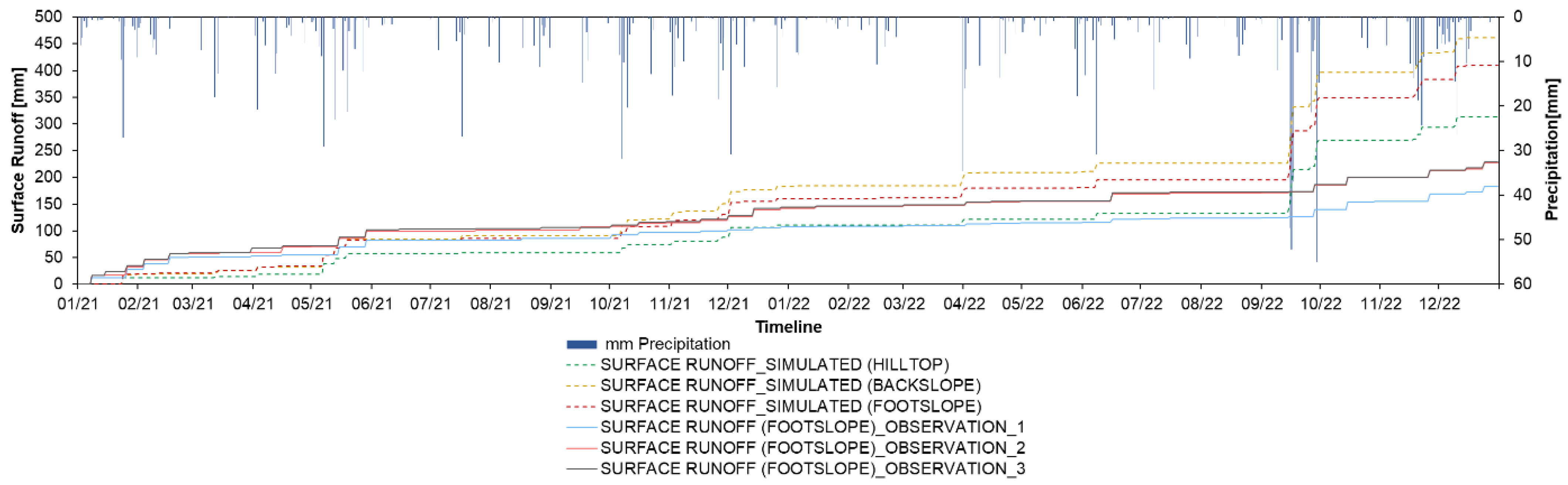
3.2. Lysimeter Outflows and Surface Runoff Observations
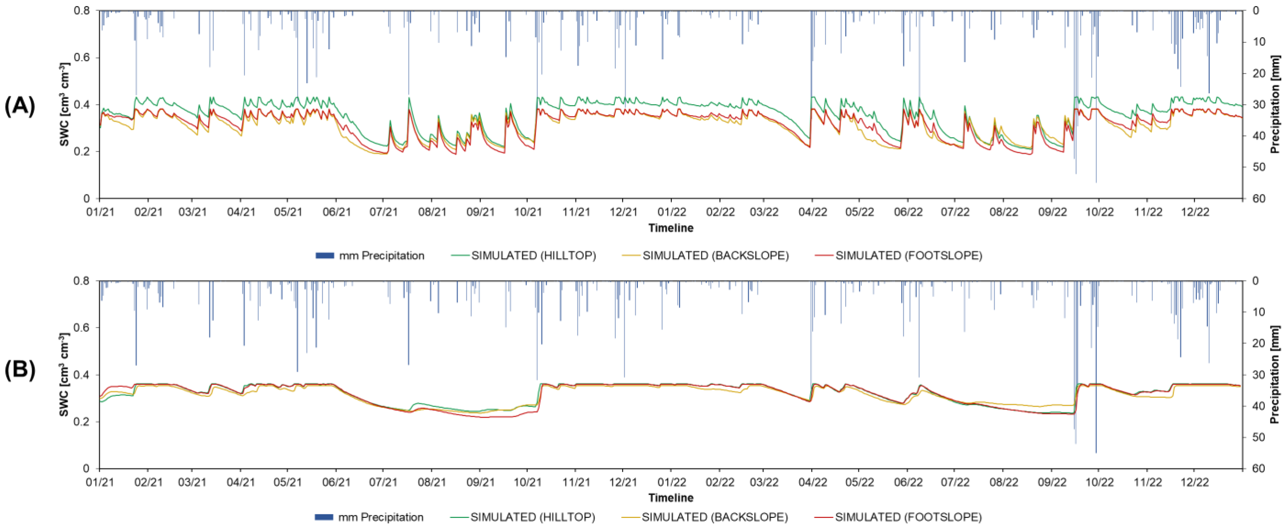
3.3. Numerical Simulations of Soil–Water Fluxes
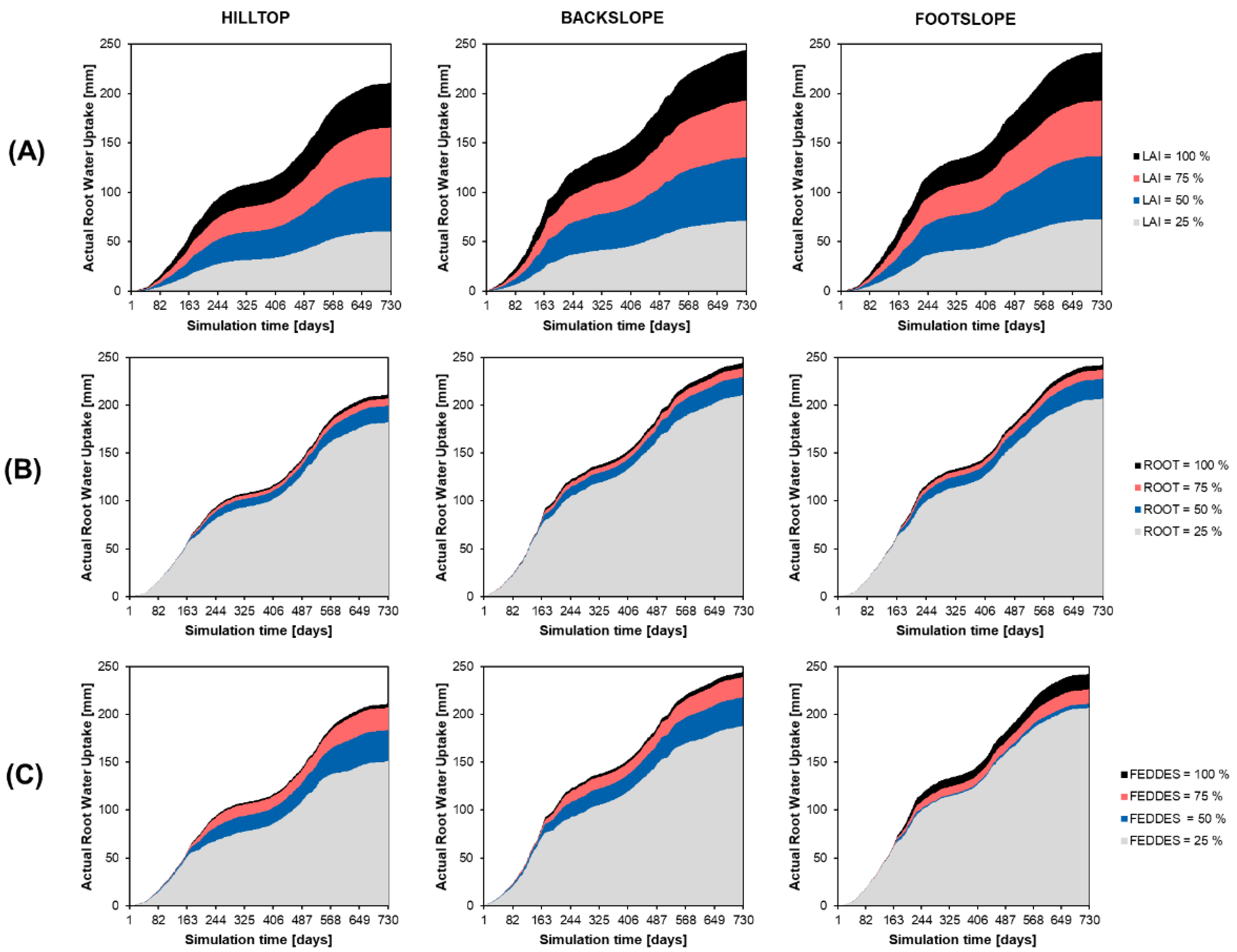
3.4. Sensitivity Analysis for RWU Parameters
4. Discussion
5. Conclusions
Author Contributions
Funding
Data Availability Statement
Conflicts of Interest
References
- Needelman, B.A.; Gburek, W.J.; Petersen, G.W.; Sharpley, A.N.; Kleinman, P.J.A. Surface Runoff along Two Agricultural Hillslopes with Contrasting Soils. Soil Sci. Soc. Am. J. 2004, 68, 914. [Google Scholar] [CrossRef]
- Rodrigo Comino, J.; Senciales, J.M.; Ramos, M.C.; Martínez-Casasnovas, J.A.; Lasanta, T.; Brevik, E.C.; Ries, J.B.; Ruiz Sinoga, J.D. Understanding soil erosion processes in Mediterranean sloping vineyards (Montes de Málaga, Spain). Geoderma 2017, 296, 47–59. [Google Scholar] [CrossRef]
- Scherrer, S.; Naef, F.; Fach, A.O.; Cordery, I. Formation of runoff at the hillslope scale during intense precipitation. Hydrol. Earth Syst. Sci. 2007, 11, 907–922. [Google Scholar] [CrossRef]
- Zhang, Y.; Huang, M. Spatial variability and temporal stability of actual evapotranspiration on a hillslope of the Chinese Loess Plateau. J. Arid Land 2021, 13, 189–204. [Google Scholar] [CrossRef]
- Zhu, B.; Wang, T.; Kuang, F.; Luo, Z.; Tang, J.; Xu, T. Measurements of Nitrate Leaching from a Hillslope Cropland in the Central Sichuan Basin, China. Soil Sci. Soc. Am. J. 2009, 73, 1419–1426. [Google Scholar] [CrossRef]
- Yang, X.; Leys, J.; Gray, J.; Zhang, M. Hillslope erosion improvement targets: Towards sustainable land management across New South Wales, Australia. CATENA 2022, 211, 105956. [Google Scholar] [CrossRef]
- Arboleda Obando, P.F.; Ducharne, A.; Cheruy, F.; Jost, A.; Ghattas, J.; Colin, J.; Nous, C. Influence of Hillslope Flow on Hydroclimatic Evolution Under Climate Change. Earth’s Futur. 2022, 10, 24. [Google Scholar] [CrossRef]
- Bryan, R.B. Soil erodibility and processes of water erosion on hillslope. Geomorphology 2000, 32, 385–415. [Google Scholar] [CrossRef]
- Coblinski, J.A.; Favaretto, N.; Goularte, G.D.; Dieckow, J.; de Moraes, A.; de Paula Souza, L.C. Water, Soil and Nutrients Losses by Runoff at Hillslope Scale in Agricultural and Pasture Production in Southern Brazil. J. Agric. Sci. 2019, 11, 160. [Google Scholar] [CrossRef]
- Vanden Heuvel, J.; Centinari, M. Under-Vine Vegetation Mitigates the Impacts of Excessive Precipitation in Vineyards. Front. Plant Sci. 2021, 12, 713135. [Google Scholar] [CrossRef]
- Kahimba, F.C.; Ranjan, R.S.; Froese, J.; Entz, M.; Nason, R. Crop cover effects on infiltration, soil temperature, and soil moisture distribution in the Canadian Prairies. Appl. Eng. Agric. 2008, 24, 321–334. [Google Scholar] [CrossRef]
- Dong, Y.; Lei, T.; Li, S.; Yuan, C.; Zhou, S.; Yang, X. Effects of rye grass coverage on soil loss from loess slopes. Int. Soil Water Conserv. Res. 2015, 3, 170–182. [Google Scholar] [CrossRef]
- Zemke, J.J.; Enderling, M.; Klein, A.; Skubski, M. The influence of soil compaction on runoff formation. A case study focusing on skid trails at forested andosol sites. Geosciences 2019, 9, 204. [Google Scholar] [CrossRef]
- Bogunovic, I.; Bilandzija, D.; Andabaka, Z.; Stupic, D.; Rodrigo Comino, J.; Cacic, M.; Brezinscak, L.; Maletic, E.; Pereira, P. Soil compaction under different management practices in a Croatian vineyard. Arab. J. Geosci. 2017, 10, 340. [Google Scholar] [CrossRef]
- Linares, R.; de la Fuente, M.; Junquera, P.; Lissarrague, J.R.; Baeza, P. Effects of soil management in vineyard on soil physical and chemical characteristics. BIO Web Conf. 2014, 3, 01008. [Google Scholar] [CrossRef]
- Li, Q.; Wei, M.; Li, Y.; Feng, G.; Wang, Y.; Li, S.; Zhang, D. Effects of soil moisture on water transport, photosynthetic carbon gain and water use efficiency in tomato are influenced by evaporative demand. Agric. Water Manag. 2019, 226, 105818. [Google Scholar] [CrossRef]
- Kang, S.; Zhang, L.; Liang, Y.; Hu, X.; Cai, H.; Gu, B. Effects of limited irrigation on yield and water use efficiency of winter wheat in the Loess Plateau of China. Agric. Water Manag. 2002, 55, 203–216. [Google Scholar] [CrossRef]
- Celette, F.; Findeling, A.; Gary, C. Competition for nitrogen in an unfertilized intercropping system: The case of an association of grapevine and grass cover in a Mediterranean climate. Eur. J. Agron. 2009, 30, 41–51. [Google Scholar] [CrossRef]
- Shen, J.; Hoffland, E. In situ sampling of small volumes of soil solution using modified micro-suction cups. Plant Soil 2007, 292, 161–169. [Google Scholar] [CrossRef]
- Schmidt, J.P.; Lin, H. Water and bromide recovery in wick and pan lysimeters under conventional and zero tillage. Commun. Soil Sci. Plant Anal. 2008, 39, 108–123. [Google Scholar] [CrossRef]
- Groh, J.; Stumpp, C.; Lücke, A.; Pütz, T.; Vanderborght, J.; Vereecken, H. Inverse Estimation of Soil Hydraulic and Transport Parameters of Layered Soils from Water Stable Isotope and Lysimeter Data. Vadose Zone J. 2018, 17, 170168. [Google Scholar] [CrossRef]
- Groffman, P.M.; Williams, C.O.; Pouyat, R.V.; Band, L.E.; Yesilonis, I.D. Nitrate Leaching and Nitrous Oxide Flux in Urban Forests and Grasslands. J. Environ. Qual. 2009, 38, 1848–1860. [Google Scholar] [CrossRef] [PubMed]
- Filipović, V.; Kodešová, R.; Petošić, D. Experimental and mathematical modeling of water regime and nitrate dynamics on zero tension plate lysimeters in soil influenced by high groundwater table. Nutr. Cycl. Agroecosyst. 2013, 95, 23–42. [Google Scholar] [CrossRef]
- Tiefenbacher, A.; Weigelhofer, G.; Klik, A.; Pucher, M.; Santner, J.; Wenzel, W.; Eder, A.; Strauss, P. Short-term effects of fertilization on dissolved organic matter in soil leachate. Water 2020, 12, 1617. [Google Scholar] [CrossRef]
- Holder, M.; Brown, K.W.; Thomas, J.C.; Zabcik, D.; Murray, H.E. Capillary-Wick Unsaturated Zone Soil Pore Water Sampler. Soil Sci. Soc. Am. J. 1991, 55, 1195–1202. [Google Scholar] [CrossRef]
- Filipović, V.; Coquet, Y.; Pot, V.; Houot, S.; Benoit, P. Modeling the effect of soil structure on water flow and isoproturon dynamics in an agricultural field receiving repeated urban waste compost application. Sci. Total Environ. 2014, 499, 546–559. [Google Scholar] [CrossRef]
- Ben-Gal, A.; Shani, U. A highly conductive drainage extension to control the lower boundary condition of lysimeters. Plant Soil 2002, 239, 9–17. [Google Scholar] [CrossRef]
- Wessel-Bothe, S.; Weihermüller, L. (Eds.) Field Measurement Methods in Soil Science; Borntraeger Gebrueder: Stuttgart, Germany, 2020. [Google Scholar]
- Stewart, R.D.; Liu, Z.; Rupp, D.E.; Higgins, C.W.; Selker, J.S. A new instrument to measure plot-scale runoff. Geosci. Instrum. Methods Data Syst. 2015, 4, 57–64. [Google Scholar] [CrossRef]
- Szilagyi, J. Analysis of the nonlinearity in the hillslope runoff response to precipitation through numerical modeling. J. Hydrol. 2007, 337, 391–401. [Google Scholar] [CrossRef]
- Fan, Y.; Clark, M.; Lawrence, D.M.; Swenson, S.; Band, L.E.; Brantley, S.L.; Brooks, P.D.; Dietrich, W.E.; Flores, A.; Grant, G.; et al. Hillslope Hydrology in Global Change Research and Earth System Modeling. Water Resour. Res. 2019, 55, 1737–1772. [Google Scholar] [CrossRef]
- Filipović, V.; Defterdarović, J.; Krevh, V.; Filipović, L.; Ondrašek, G.; Kranjčec, F.; Magdić, I.; Rubinić, V.; Stipičević, S.; Mustać, I.; et al. Estimation of stagnosol hydraulic properties and water flow using uni-and bimodal porosity models in erosion-affected hillslope vineyard soils. Agronomy 2022, 12, 33. [Google Scholar] [CrossRef]
- Vereecken, H.; Schnepf, A.; Hopmans, J.W.; Javaux, M.; Or, D.; Roose, T.; Vanderborght, J.; Young, M.H.; Amelung, W.; Aitkenhead, M.; et al. Modeling Soil Processes: Review, Key Challenges, and New Perspectives. Vadose Zone J. 2016, 15, 1–57. [Google Scholar] [CrossRef]
- Ritter, A.; Hupet, F.; Muñoz-Carpena, R.; Lambot, S.; Vanclooster, M. Using inverse methods for estimating soil hydraulic properties from field data as an alternative to direct methods. Agric. Water Manag. 2003, 59, 77–96. [Google Scholar] [CrossRef]
- Filipović, V.; Weninger, T.; Filipović, L.; Schwen, A.; Bristow, K.L.; Zechmeister-Boltenstern, S.; Leitner, S. Inverse estimation of soil hydraulic properties and water repellency following artificially induced drought stress. J. Hydrol. Hydromech. 2018, 66, 170–180. [Google Scholar] [CrossRef]
- Namitha, M.R.; Ravikumar, V. Determination of Unsaturated Hydraulic Conductivity in Field Conditions through Inverse Modelling Using Hydrus-ID. Int. J. Sci. Eng. Manag. 2017, 2, 50–57. [Google Scholar]
- Zhang, K.; Burns, I.G.; Greenwood, D.J.; Hammond, J.P.; White, P.J. Developing a reliable strategy to infer the effective soil hydraulic properties from field evaporation experiments for agro-hydrological models. Agric. Water Manag. 2010, 97, 399–409. [Google Scholar] [CrossRef]
- Kuhl, A.S.; Kendall, A.D.; Van Dam, R.L.; Hyndman, D.W. Quantifying Soil Water and Root Dynamics Using a Coupled Hydrogeophysical Inversion. Vadose Zone J. 2018, 17, 1–13. [Google Scholar] [CrossRef]
- Hupet, F.; Lambot, S.; Feddes, R.A.; Van Dam, J.C.; Vanclooster, M. Estimation of root water uptake parameters by inverse modeling with soil water content data. Water Resour. Res. 2003, 39, 1312. [Google Scholar] [CrossRef]
- Zeng, W.; Lei, G.; Zha, Y.; Fang, Y.; Wu, J.; Huang, J. Sensitivity and uncertainty analysis of the HYDRUS-1D model for root water uptake in saline soils. Crop Pasture Sci. 2018, 69, 163–173. [Google Scholar] [CrossRef]
- Cai, G.; Vanderborght, J.; Couvreur, V.; Mboh, C.M.; Vereecken, H. Parameterization of Root Water Uptake Models Considering Dynamic Root Distributions and Water Uptake Compensation. Vadose Zone J. 2018, 17, 1–21. [Google Scholar] [CrossRef]
- International Union of Soil Sciences (IUSS) Working Group WRB. International Soil Classification System for Naming Soils and Creating Legends for Soil Maps, 4th ed.; IUSS: Vienna, Austria, 2022; ISBN 9798986245119. [Google Scholar]
- Krevh, V.; Groh, J.; Weihermüller, L.; Filipović, L.; Defterdarović, J.; Kovač, Z.; Magdić, I.; Lazarević, B.; Baumgartl, T.; Filipović, V. Investigation of Hillslope Vineyard Soil Water Dynamics Using Field Measurements and Numerical Modeling. Water 2023, 15, 820. [Google Scholar] [CrossRef]
- METER. HYPROP Manual; UMS: Munich, Germany, 2015. [Google Scholar]
- METER. WP4C Manual; METER: Pullman, WA, USA, 2021. [Google Scholar]
- METER. HYPROP-FIT User’s Manual; METER: Pullman, WA, USA, 2015. [Google Scholar]
- Šimůnek, J.; Bradford, S.A. Vadose Zone Modeling: Introduction and Importance. Vadose Zone J. 2008, 7, 581–586. [Google Scholar] [CrossRef]
- Šimůnek, J.; van Genuchten, M.T.; Šejna, M. Recent Developments and Applications of the HYDRUS Computer Software Packages. Vadose Zone J. 2016, 15, 1–25. [Google Scholar] [CrossRef]
- Van Genuchten, M.T. A closed-form equation for predicting the hydraulic conductivity of unsaturated soils. Soil Sci. Soc. Am. J. 1980, 44, 892–898. [Google Scholar] [CrossRef]
- Mualem, Y. A New Model for Predicting the Hydraulic Conductivity of Unsaturated Porous Media. Water Resour. Res. 1976, 12, 513–522. [Google Scholar] [CrossRef]
- Allen, R.G.; Pruitt, W.O.; Wright, J.L.; Howell, T.A.; Ventura, F.; Snyder, R.; Itenfisu, D.; Steduto, P.; Berengena, J.; Yrisarry, J.B.; et al. A recommendation on standardized surface resistance for hourly calculation of reference ETo by the FAO56 Penman-Monteith method. Agric. Water Manag. 2006, 81, 1–22. [Google Scholar] [CrossRef]
- Gebler, S.; Hendricks Franssen, H.J.; Pütz, T.; Post, H.; Schmidt, M.; Vereecken, H. Actual evapotranspiration and precipitation measured by lysimeters: A comparison with eddy covariance and tipping bucket. Hydrol. Earth Syst. Sci. 2015, 19, 2145–2161. [Google Scholar] [CrossRef]
- Feddes, R.A.; Kowalik, P.J.; Zaradny, H. Simulation of Field Water Use and Crop Yield; Simulation Monographs; Centre for Agricultural Publishing and Documentation: Wageningen, The Netherlands, 1978. [Google Scholar]
- Liu, L.; Yu, H. A sensitivity analysis of simulated infiltration rates to uncertain discretization in the moisture content domain. Water 2019, 11, 1192. [Google Scholar] [CrossRef]
- Marquardt, D.W. An Algorithm for Least-Squares Estimation of Nonlinear Parameters. J. Soc. Ind. Appl. Math. 1963, 11, 431–441. [Google Scholar] [CrossRef]
- Kool, J.B.; Parker, J.C.; van Genuchten, M.T. Determining Soil Hydraulic Properties from One-step Outflow Experiments by Parameter Estimation: I. Theory and Numerical Studies. Soil Sci. Soc. Am. J. 1985, 49, 1348–1354. [Google Scholar] [CrossRef]
- Kool, J.B.; Parker, J.C.; van Genuchten, M.T. Parameter estimation for unsaturated flow and transport models—A review. J. Hydrol. 1987, 91, 255–293. [Google Scholar] [CrossRef]
- Šimůnek, J.; Angulo-Jaramillo, R.; Schaap, M.G.; Vandervaere, J.P.; Van Genuchten, M.T. Using an inverse method to estimate the hydraulic properties of crusted soils from tension-disc infiltrometer data. Geoderma 1998, 86, 61–81. [Google Scholar] [CrossRef]
- González, M.G.; Ramos, T.B.; Carlesso, R.; Paredes, P.; Petry, M.T.; Martins, J.D.; Aires, N.P.; Pereira, L.S. Modelling soil water dynamics of full and deficit drip irrigated maize cultivated under a rain shelter. Biosyst. Eng. 2015, 132, 1–18. [Google Scholar] [CrossRef]
- Yang, Y.; Chen, R.S.; Song, Y.X.; Han, C.T.; Liu, Z.W.; Liu, J.F. Spatial variability of soil hydraulic conductivity and runoff generation types in a small mountainous catchment. J. Mt. Sci. 2020, 17, 2724–2741. [Google Scholar] [CrossRef]
- Yang, J.; Yu, Z.; Yi, P.; Frape, S.K.; Gong, M.; Zhang, Y. Evaluation of surface water and groundwater interactions in the upstream of Kui river and Yunlong lake, Xuzhou, China. J. Hydrol. 2020, 583, 124549. [Google Scholar] [CrossRef]
- Assouline, S. Infiltration into soils: Conceptual approaches and solutions. Water Resour. Res. 2013, 49, 1755–1772. [Google Scholar] [CrossRef]
- Lisboa, M.S.; Schneider, R.L.; Sullivan, P.J.; Walter, M.T. Drought and post-drought rain effect on stream phosphorus and other nutrient losses in the Northeastern USA. J. Hydrol. Reg. Stud. 2020, 28, 100672. [Google Scholar] [CrossRef]
- Sandi, S.G.; Rodriguez, J.F.; Saintilan, N.; Wen, L.; Kuczera, G.; Riccardi, G.; Saco, P.M. Resilience to drought of dryland wetlands threatened by climate change. Sci. Rep. 2020, 10, 13232. [Google Scholar] [CrossRef]
- Qiu, J.; Shen, Z.; Leng, G.; Wei, G. Synergistic effect of drought and rainfall events of different patterns on watershed systems. Sci. Rep. 2021, 11, 18957. [Google Scholar] [CrossRef]
- Geneti, T.Z. Review on the Effect of Moisture or Rain Fall on Crop Production. Civ. Environ. Res. 2019, 11, 1–7. [Google Scholar] [CrossRef]
- Ojo, O.I.; Ilunga, M.F. The Rainfall Factor of Climate Change Effects on the Agricultural Environment: A Review. Am. J. Appl. Sci. 2017, 14, 930–937. [Google Scholar] [CrossRef]
- Horel, Á.; Zsigmond, T. Plant Growth and Soil Water Content Changes under Different Inter-Row Soil Management Methods in a Sloping Vineyard. Plants 2023, 12, 1549. [Google Scholar] [CrossRef] [PubMed]
- Haruna, S.I.; Eichas, R.C.; Peters, O.M.; Farmer, A.C.; Lackey, D.Q.; Nichols, J.E.; Peterson, W.H.; Slone, N.A. In situ water infiltration: Influence of cover crops after growth termination. Soil Sci. Soc. Am. J. 2022, 86, 769–780. [Google Scholar] [CrossRef]
- Chahinian, N.; Voltz, M.; Moussa, R.; Trotoux, G. Assessing the impactof the hydraulic properties of a crusted soil on overland flow modelling at the field scale. Hydrol. Process. 2006, 20, 1701–1722. [Google Scholar] [CrossRef]
- Martínez-Fernández, J.; González-Zamora, A.; Almendra-Martín, L. Soil moisture memory and soil properties: An analysis with the stored precipitation fraction. J. Hydrol. 2021, 593, 125622. [Google Scholar] [CrossRef]
- Martínez-De La Torre, A.; Miguez-Macho, G. Groundwater influence on soil moisture memory and land-atmosphere fluxes in the Iberian Peninsula. Hydrol. Earth Syst. Sci. 2019, 23, 4909–4932. [Google Scholar] [CrossRef]
- Cai, F.; Ming, H.; Mi, N.; Xie, Y.; Zhang, Y.; Li, R. Effects of optimized root water uptake parameterization schemes on water and heat flux simulation in a maize agroecosystem. J. Meteorol. Res. 2017, 31, 363–377. [Google Scholar] [CrossRef]
- Angaleeswari, M.; Ravikumar, V. Estimating root water uptake parameters by inverse modelling. Agric. Water Manag. 2019, 223, 105681. [Google Scholar] [CrossRef]


| Position on the Hillslope | Depth [cm] | Sand (%) (2–0.063) | SD | Silt (%) (0.063–0.02) | SD | Clay (%) | SD | SOC [g kg−1] |
|---|---|---|---|---|---|---|---|---|
| Hilltop | 0–30 | 5.7 | 1.5 | 71.0 | 1.0 | 23.3 | 0.6 | 12.0 |
| Backslope | 6.7 | 0.6 | 70.0 | 1.0 | 23.3 | 0.6 | 9.8 | |
| Footslope | 6.7 | 1.5 | 75.0 | 3.0 | 18.3 | 4.5 | 12.4 | |
| Hilltop | 30–60 | 4.7 | 1.2 | 69.0 | 2.0 | 26.3 | 1.2 | 5.9 |
| Backslope | 8.3 | 3.2 | 67.3 | 3.1 | 24.3 | 1.5 | 6.1 | |
| Footslope | 7.0 | 0.0 | 72.0 | 6.0 | 21.0 | 6.0 | 8.1 |
| Position | Depth (cm) | θr (cm3 cm−3) | θs (cm3 cm−3) | α (cm−1) | n (-) | Ks (cm day−1) | Ksopt (cm day−1) | RMSE (θ) | BD (g cm −3) |
|---|---|---|---|---|---|---|---|---|---|
| Hilltop | 0–20 | 0.000 * | 0.432 | 0.00379 | 1.219 | 0.31 | 1.14 | 0.0219 | 1.48 |
| 20–40 | 0.000 * | 0.386 | 0.00610 | 1.172 | 1.37 | 10.36 | 0.0167 | 1.52 | |
| Backslope | 0–20 | 0.000 * | 0.38 | 0.00413 | 1.205 | 0.33 | 0.79 | 0.0136 | 1.60 |
| 20–40 | 0.000 * | 0.373 | 0.00432 | 1.199 | 1.20 | 1.20 | 0.0183 | 1.54 | |
| Footslope | 0–20 | 0.000 * | 0.382 | 0.00399 | 1.22 | 0.45 | 0.93 | 0.0143 | 1.51 |
| 20–40 | 0.000 * | 0.381 | 0.00432 | 1.223 | 0.60 | 1.68 | 0.0129 | 1.54 |
| Observation | Position | 2021 | 2022 | ||||||
|---|---|---|---|---|---|---|---|---|---|
| Winter | Spring | Summer | Autumn | Winter | Spring | Summer | Autumn | ||
| Lysimeter outflow | Hilltop | 112.4 | 74.6 | 1.3 | 52.5 | 30.4 | 17.9 | 21.5 | 44.0 |
| Backslope | 34.9 | 31.7 | 0.2 | 31.0 | 39.6 | 12.9 | 18.5 | 39.0 | |
| Footslope | 119.7 | 51.5 | 0.4 | 30.6 | 15.0 | 3.1 | 14.6 | 64.6 | |
| Surface runoff | Footslope | 57.2 | 37.3 | 9.2 | 27.7 | 8.3 | 14.4 | 16.4 | 42.4 |
| Simulations | Parameter | Hilltop | Backslope | Footslope |
|---|---|---|---|---|
| Initial run | R2 | 0.90 | 0.90 | 0.89 |
| RMSE | 183.81 | 83.64 | 106.76 | |
| NSE | −4.14 | −1.27 | −2.33 | |
| Optimized run | R2 | 0.94 | 0.95 | 0.92 |
| RMSE | 51.63 | 17.71 | 46.25 | |
| NSE | 0.59 | 0.90 | 0.38 |
| Position | Footslope | |||
|---|---|---|---|---|
| Simulations | Parameter | Observation_1 | Observation_2 | Observation_3 |
| 2021 | R2 | 0.88 | 0.92 | 0.92 |
| RMSE | 20.8 | 21.9 | 23.6 | |
| NSE | 0.52 | 0.65 | 0.60 | |
| 2022 | R2 | 0.97 | 0.93 | 0.93 |
| RMSE | 122.7 | 88.5 | 87.6 | |
| NSE | −29.8 | −12.5 | −12.2 | |
Disclaimer/Publisher’s Note: The statements, opinions and data contained in all publications are solely those of the individual author(s) and contributor(s) and not of MDPI and/or the editor(s). MDPI and/or the editor(s) disclaim responsibility for any injury to people or property resulting from any ideas, methods, instructions or products referred to in the content. |
© 2023 by the authors. Licensee MDPI, Basel, Switzerland. This article is an open access article distributed under the terms and conditions of the Creative Commons Attribution (CC BY) license (https://creativecommons.org/licenses/by/4.0/).
Share and Cite
Krevh, V.; Filipović, L.; Defterdarović, J.; Bogunović, I.; Zhang, Y.; Kovač, Z.; Barton, A.; Filipović, V. Investigating Near-Surface Hydrologic Connectivity in a Grass-Covered Inter-Row Area of a Hillslope Vineyard Using Field Monitoring and Numerical Simulations. Land 2023, 12, 1095. https://doi.org/10.3390/land12051095
Krevh V, Filipović L, Defterdarović J, Bogunović I, Zhang Y, Kovač Z, Barton A, Filipović V. Investigating Near-Surface Hydrologic Connectivity in a Grass-Covered Inter-Row Area of a Hillslope Vineyard Using Field Monitoring and Numerical Simulations. Land. 2023; 12(5):1095. https://doi.org/10.3390/land12051095
Chicago/Turabian StyleKrevh, Vedran, Lana Filipović, Jasmina Defterdarović, Igor Bogunović, Yonggen Zhang, Zoran Kovač, Andrew Barton, and Vilim Filipović. 2023. "Investigating Near-Surface Hydrologic Connectivity in a Grass-Covered Inter-Row Area of a Hillslope Vineyard Using Field Monitoring and Numerical Simulations" Land 12, no. 5: 1095. https://doi.org/10.3390/land12051095