A Study on the Spatial and Temporal Variation of Summer Surface Temperature in the Bosten Lake Basin and Its Influencing Factors

Abstract

The land surface temperature (LST) is an important indicator reflecting the ecological environment condition. As a sensitive area to climate change, mastering the spatial and temporal changes of summer LST in the Bosten Lake basin (BLB) helps gain insight into the evolution of the thermal environment in the Bosten Lake basin and for long-term monitoring of the basic ecological changes in the basin. Based on MOD11A1 data from 2005 to 2020, this paper investigates the diurnal LST spatiotemporal series variation and its influencing factors in the Bosten Lake basin by using surface temperature class classification, trending analysis, the Hurst index, and geographic probes. The results show that (1) the wetland grasslands in and around the Bayinbruck steppe in the northwestern part of the study area exhibit a heat island effect during the day, while the opposite is true at night. In terms of temporal changes, LST changes in the BLB fluctuate widely, having a general rising and then decreasing trend. (2) The decreasing trend of LST from 2005 to 2020 is significant during the daytime and vice versa at night, and the change at night is greater than during the day. The areas with significantly higher diurnal LST in the future have all expanded compared to the area occupied by them now, with an overall trend of a steady increase. (3) The dominant factor of LST variation has the strongest explanatory power when altitude and NDVI are combined during the daytime and the strongest explanatory power when NPP and temperature are combined at night.

1. Introduction

Land surface temperature (LST) is an important parameter for exploring surface radiation, surface energy balance processes, and the most direct manifestation of the thermal environment [1]. The sixth IPCC report states that under 2 °C and 4 °C warming scenarios, 3–4 billion people globally will face physical water scarcity; 42–79% of global watershed runoff will be affected by 2050, adversely affecting freshwater ecosystems [2]. With the evolution of spatial patterns of surface warming, global climate change patterns are becoming more complex, and regional surface temperature changes in the context of climate warming have become the focus of pressing ecological issues nowadays [3]. Surface temperature, as an important parameter widely used in several research fields, such as geology [4], ecology [5], meteorology [6], and agronomy [7], is important for the maintenance of biodiversity, diversification of agricultural production, and human survival and development. In the natural substratum, the decrease in soil water content caused by the increase in surface temperature can cause water stress to the growth of vegetation [8]. The rise in surface temperature negatively affects vegetation that is sensitive to temperature changes, thus causing various environmental problems [9]. In the anthropogenic property subsurface, the surface temperature can significantly affect the regional climate of the human settlement [10]. The joint impact of surface temperature on the natural environment and human society determines its importance for the study of global ecosystems [11], modern agriculture [12], and urbanization development [13].

Because of the advancement and use of remote sensing technology, the quantitative inversion of remote sensing based on various satellite data (Landsat, MODIS, AVHRR, ASTER, etc.) has provided a new way for the rapid acquisition of large-scale, space–time continuous LST. Among them, MODIS surface temperature products can meet the requirements of large- and medium-scale studies [14,15], and the good results achieved in the areas affected by climate, such as Tianshan [16] and the Qinghai–Tibet Plateau [17], indicate that the data products have the more scientific and reliable characterization of surface energy under complex terrain. Current research methods on surface temperature focus on (1) split-window algorithms applied to ASTER data [18]. (2) A time series harmonic analysis [19] was used in the reconstruction of time series images of the LST to explore interannual variability, peak cycles, and seasonal fluctuations in LST. (3) For driving force analysis of LST, a large number of studies have used ordinary linear regression or geographically weighted regression [20] to explore the combined effects of multiple influencing factors on surface temperature. The current research hotspots are mainly the spatial and temporal variation of LST in regions such as Beijing [21], Pearl River [22], the Qinghai–Tibet Plateau [23], and Tian Shan [24], but the spatial and temporal variation patterns of natural attribute subsurface temperature in the arid and semi-arid regions of northwest China are less studied.

The Bosten Lake basin (BLB) is located deeply inland in the northwest, with complex land use types, and is an important natural property substrate for regulating the regional climate in Xinjiang. As the largest inland freshwater lake in China, Bosten Lake plays a key role in the ecological construction of the lower Tarim River. It has been shown that changes in surface temperature can alter the material and energy balance between the ground and the atmosphere, resulting in changes in important ecological parameters such as evapotranspiration, temperature, precipitation, and vegetation [25], which in turn have an important impact on the conservation and evolution of the regional ecological environment. At present, significant results have been achieved in the study of the natural ecology of the BLB, mainly focusing on climate change, land use/cover change, and water resource change [26,27,28]. Sen’s slope analysis and linear trend analysis are commonly used in the study of surface temperature time series data analysis. Linear trend analysis is used to fit the time series data using methods such as least squares [29], and then judge the trend based on the results of the fit, which is a simpler and more intuitive method, but it is difficult to ignore the effects of missing values and outliers. In contrast, Sen’s slope analysis is a robust trend calculation method with nonparametric statistics [30], which is computationally efficient, insensitive to measurement errors and outlier data, and suitable for trend analysis of long time series data. Therefore, this study uses the BLB as the study area to investigate the long time series of surface temperature; this serves as a scientific foundation for the region’s sustainable development and ecological preservation.

2. Materials and Methods

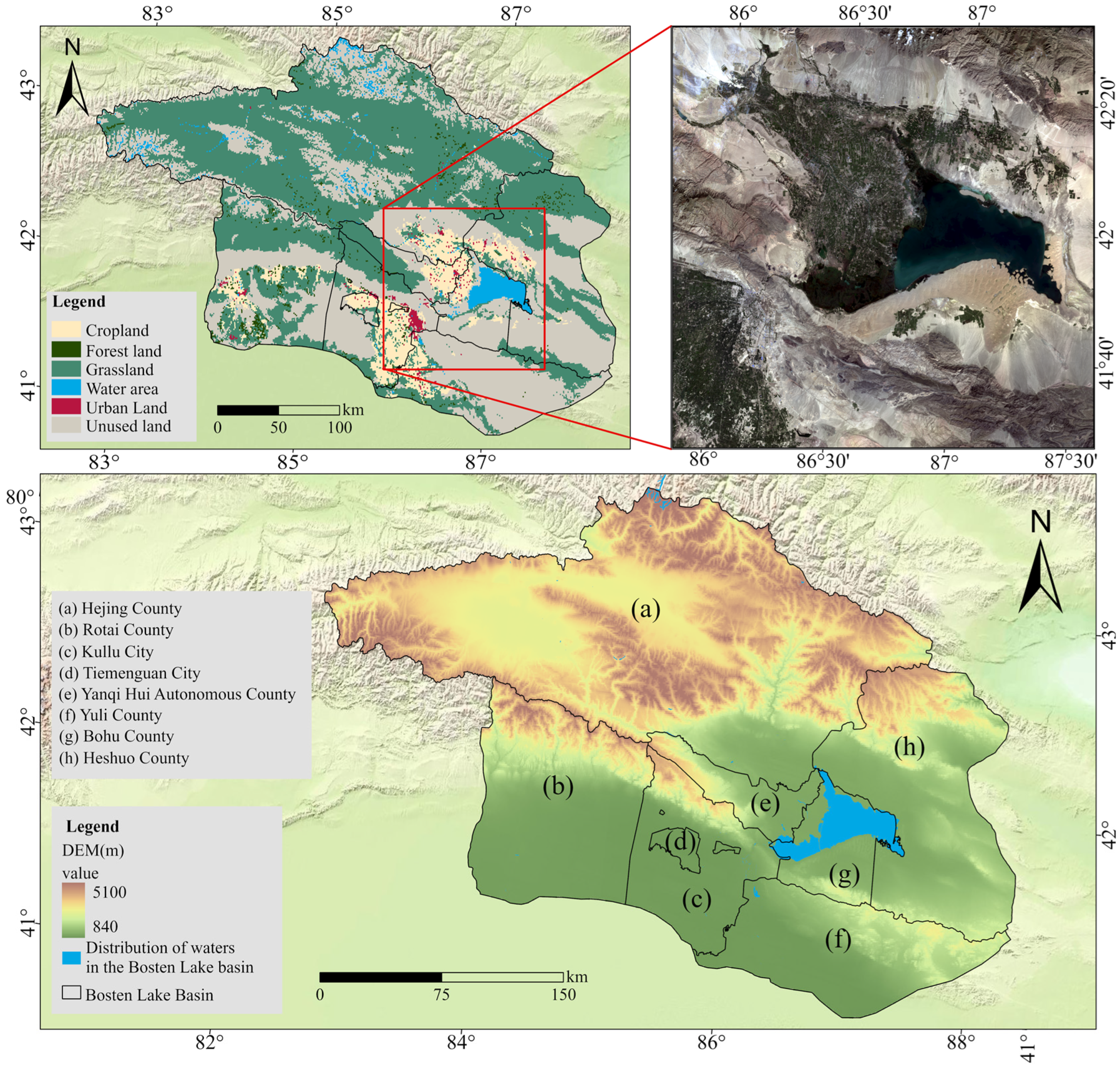
2.1. Study Area

In this paper, the BLB was selected as the study area (Figure 1), which is located in the south of the Tianshan Mountains in Bayingoleng Mongol Autonomous Prefecture, Xinjiang Uygur Autonomous Region, northwestern China, between 82°57′ and 88°18′ E and 41°25′ and 43°34′ N, with a watershed area of about 79,204.25 km². The topography of this region is high in the north and low in the south and high in the west and low in the east, with mountains, canyons, and basins crisscrossing the area, and the terrain is extremely complex. Bosten Lake is the largest inland freshwater lake in China and the origin of the Peacock River [31]. The whole area of the BLB includes Heshuo County, Hejing County, Yanqi County, Bohu County, Luntai County (part of it), Kulle City, Tiemenguan City (formerly the Second Division of Xinjiang Production and Construction Corps), and part of Yuli County. The Bosten Lake basin has a temperate continental arid climate. The average annual temperature ranges between 8.2 and 11.5 °C and the average annual precipitation is only about 60 mm, while the evaporation is higher than 2000 mm. The water bodies of Bosten Lake are strongly influenced by surface temperature and anthropogenic factors, so the study of surface temperature in the BLB has important theoretical significance and practical value for the sustainable socio-economic development of the basin and even the healthy development of the Tarim River ecosystem.

2.2. Data Sources

First, this study uses the average 8-day synthetic diurnal temperature difference product MOD11A1 data downloaded from NASA (https://ladsweb.modaps.eosdis.nasa.gov/, accessed on 10 September 2022) for the Aqua satellite from June 2005 to August 2020. The MOD11A1 product includes both daytime and nighttime LST datasets. The daytime LST is observed at 10:30 A.M. each day to reflect the daytime LST of that day. The nighttime LST is observed at 10:30 P.M. each day to reflect the nighttime LST of that day. Because the daytime and nighttime LSTs are affected by different factors, such as solar radiation and temperature, they are observed and extracted separately, and the data are reprojected using the official MODIS Reprojection Tool (MRT) and mosaic. The normalized difference vegetation index (NDVI) data for 2020 were obtained from NASA’s MODIS vegetation index product MYD13A2. Altitude, gradient, precipitation, land-use/land-cover (LULC), AOD, GDP, air temperature, and net primary productivity (NPP) data were from the Chinese Academy of Sciences Resource and Environment Science Data Center (https://www.resdc.cn/ (accessed on 10 September 2022)).

Table 1. Details and sources of influencing factors.

Types of Influencing Factors	Influencing Factors	Spatial Resolution	Year	Access
Ground cover factors	Normalized difference vegetation index (NDVI)	1000 m	2020	https://www.nasa.gov/ (accessed on 10 September 2022)
	Land-use/land-cover (LULC)	30 m	2020	https://www.resdc.cn/ (accessed on 10 September 2022)
	Net primary production (NPP)	500 m	2020
Climate factors	Precipitation	1000 m	2020
	Air temperature	1000 m	2020
	Aerosol optical depth (AOD)	1000 m	2020
Socio-economic factors	Gross domestic product (GDP)	1000 m	2020
Terrain factors	DEM	30 m	-	http://www.gscloud.cn (accessed on 10 September 2022)
	Gradient	30 m	2020
	Altitude	30 m	2020

summarizes the details of the data for all impact factors.

2.3. Research Methodology

The framework of this study is shown in Figure 2. The diurnal LST data is used to classify the levels, analyze LST and its future trends from 2005 to 2020, and finally analyze the influencing factors of surface temperature change.

2.3.1. MODIS Data Processing

MOD11A1 data were recorded for 8 d under cloud-free conditions, and the 8 d composite LST products were calculated according to a simple averaging algorithm, with valid values ranging between 7500 and 65,535 with a conversion factor of 0.02, as queried through the LP DAAC website. MRT software was used to batch preprocess the raw MODIS data for projection conversion, band extraction, etc. Batch cropping of 144 data with the help of ArcGIS software based on the study area boundary was performed, and finally, the MODIS_LSTDE K temperature was converted to Celsius using raster calculation [32], calculated as:

$$T_s=DN\times 0.02-273.15$$

(1)

where $T_s$ denotes the surface temperature value (°C) and DN denotes the image element brightness value.

2.3.2. Land Surface Temperature Class Classification

The mean standard deviation method was used to classify the land surface temperature into five classes, and this method can well-characterize the concentration and fluctuation of temperature using a combination of mean values and different standard deviation multiples [33]. The specific land surface temperature classes are shown in

Table 2. Classification of land surface temperature.

Surface Temperature Class	Classification Range
Extremely high temperature (EHT)	$T_s>\mu +\sigma$
High temperature (HT)	$\mu +0.5\sigma <T_s\le \mu +\sigma$
Medium temperature (MT)	$\mu -0.5\sigma <T_s\le \mu +0.5\sigma$
Low temperature (LT)	$\mu -\sigma <T_s\le \mu -0.5\sigma$
Extremely low temperature (ELT)	$T_s\le \mu -\sigma$

$T_s$ is the temperature level, $\mu$ represents the mean value of surface temperature in the study area, $std$ represents the standard deviation of the surface temperature.

. Note: T is the temperature interval, μ is the mean, and std is the standard deviation.

2.3.3. Trend Analysis Method

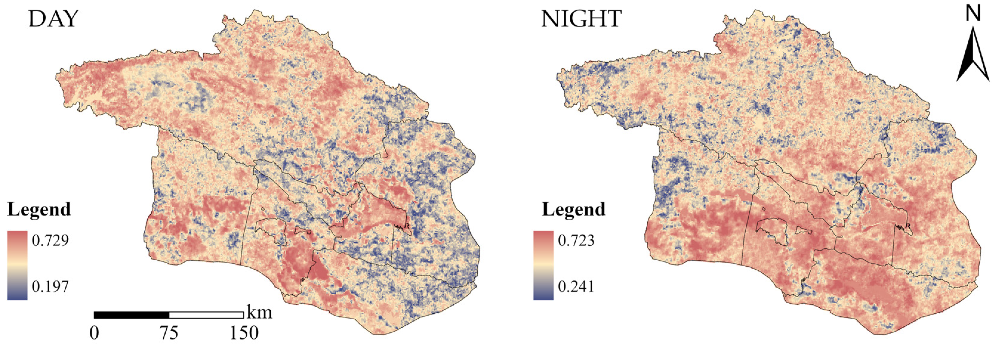
(1) Sen′s slope analysis

Sen′s slope analysis is a method to estimate the trend of the time series, and its basic principle is calculating the slope between all adjacent data in the time series and then taking the median of the slope as the trend of change, which can effectively reduce the influence of missing values and outliers [34]. The calculation formula is as follows:

$$Slope=median\left(\frac{LS{T}_j-LS{T}_i}{j-i}\right),\forall j>i$$

(2)

where the medium is the median function, $LS{T}_j$ and $LS{T}_i$ are the observations at time j and i in the time series, and $Slope$ < 0 indicates a downward trend and $Slope$ > 0 indicates an upward trend.

(2) Mann Kendal (M-K) trend test

The M-K trend test is a nonparametric test often used in conjunction with Sen′s slope analysis to determine the significance of a trend of change [35], which is used to discriminate significance by calculating its standard normal statistical distribution, Z, calculated as follows:

$$Z=\{\begin{array}{c}\frac{S-1}{\sqrt{\mathrm{Var}\left(S\right)}},S>0\\ 0,S=0\\ \frac{S+1}{\sqrt{\mathrm{Var}\left(S\right)}},S<0\end{array}$$

(3)

where Var(S) is the variance of S. The formula for S is:

$$S={\displaystyle \sum }_{i=1}^{n-1}{\displaystyle \sum }_{j=i+1}^n\mathrm{sgn}\left(LS{T}_j-LS{T}_i\right)$$

(4)

where $\mathrm{sgn}\left(LS{T}_j-LS{T}_i\right)$ is a symbolic function with the following expressions:

$$\mathrm{sgn}\left(LS{T}_j-LS{T}_i\right)=\{\begin{array}{c}1,LS{T}_j-LS{T}_i>0\\ 0,LS{T}_j-LS{T}_i=0\\ -1,LS{T}_j-LS{T}_i<0\end{array}$$

(5)

In this study, 95% and 99% confidence levels were taken, i.e., the trend of change was highly significant when Z ≥ 2.58 or Z ≤ −2.58 and significant when 1.96 ≤ Z < 2.58 or −2.58 < Z ≤ −1.96; otherwise, the trend was not significant (

Table 3. Standard of the M-K non-parametric test result classification.

Trend of Change	Statistical Quantity Z
Extremely significant reduction	Z ≤ −2.58
Significant reduction	−2.58 < Z ≤ −1.96
No significant change	−1.96 < Z ≤ 1.96
Significant increase	1.96 ≤ Z < 2.58
Extremely significant increase	Z > 2.58

).

2.3.4. Hurst Index

The Hurst index, based on rescaled polar deviation (R/S), can discern future changes in the time series by reflecting the interrelationship of the before and after time series [36]. Therefore, the combination of Sen′s slope and the M-K trend test can be used to analyze the future trend of LST. Hurst > 0.5, indicates that the LST trend is sustainable, i.e., it is highly likely that the future trend will be the same as the present; Hurst ≤ 0.5 indicates an uncertain future LST trend, which is classified as an unknown trend in this study.

To better analyze the trends of LST and future trends, this study superimposed the results of Sen’s slope analysis, the Mann Kendal trend test, and the Hurst index to analyze and classify the rank of trends. The specific division conditions are given in

Table 4. Judgment conditions and grade definitions of change trends.

Slope, Z-Value, and Hurst Index	Future Trends of Change
Slope < 0, Z ≤ −2.58, Hurst > 0.5	Continued highly significant reduction (Chsr)
Slope < 0, −2.58 < Z ≤ −1.96, Hurst > 0.5	Continued significant reduction (Csr)
Slope < 0, −1.96 < Z < 1.96, Hurst > 0.5	Sustained non-significant decrease (Snsd)
Slope > 0, 1.96 < Z < 1.96, Hurst > 0.5	Sustained non-significant elevation (Snse)
Slope > 0, 1.96 ≤ Z < 2.58, Hurst > 0.5	Continued significant elevation (Cse)
Slope > 0, Z ≥ 2.58, Hurst > 0.5	Continued highly significant elevation (Chse)
Hurst ≤ 0.5	No significant change (Nsc)

.

2.3.5. Geo-Detector Model

Geographic probes [37] are statistical models that measure heterogeneity and research drivers at the spatial level and allow for the analysis of correlations among variables without relying on linear assumptions and covariance, including factor probes, risk area probes, interaction probes, and ecological probes. In this paper, three methods, namely factor detection, interaction detection, and risk detection, are used to explore the influencing factors. Due to the availability of data, this study only uses the year 2020 as an example for the impact factor analysis. The 3km grid points are established according to the study area, and the values of each influence factor are discretized using the natural intermittent point method.

(1) Factor detection analysis

Detecting the spatial divergence of Y and detecting how much of the spatial divergence of attribute Y is explained by a certain factor X. Using the q-value metric, the expressions are:

$$q=1-\frac{{{\displaystyle \sum }}_{h=1}^L{N}_n{\sigma }_h^2}{N{\sigma }^2}=1-\frac{SSW}{SST}$$

(6)

$$SSW={{\displaystyle \sum }}_{h=1}^L{N}_h{\sigma }_h^2,SST=N{\sigma }^2$$

(7)

where h = 1,…, L is the number of partitions of each factor, i.e., the number of each subzone; N_h, N denotes the number of samples in each subregion and the total number of samples; and the value of q is [0, 1], and higher q indicates that the coefficient has a greater effect on the heat island.

(2) Interaction Detection Analysis

Identify the interaction between the different risk factors Xs and assess whether the factors X1 and X2 together increase or decrease the explanatory power of the dependent variable Y, or whether the effects of these factors on Y are independent of each other. The assessment is performed by first calculating the q-values of the two factors X1 and X2 on Y separately: q(X1) and q(X2), calculating the q-values when they interact (the new polygon distribution formed by the tangent of the two layers of the superimposed variables X1 and X2): q(X1 ∩ X2), and comparing q(X1), q(X2), and q(X1 ∩ X2).

(3) Risk Detection Analysis

Risk detection is used to determine if there is a significant difference in the mean of the attributes between the two sub-regions, and the detection effect will be tested using the t-statistic:

$$t_{{\bar{y}}_{h=1}-{\bar{y}}_{h=2}}=\frac{{\bar{Y}}_{h=1}-{\bar{Y}}_{h=2}}{{\left[\frac{\mathrm{Var}\left({\bar{Y}}_{h=1}\right)}{n_{h=1}}+\frac{\mathrm{Var}\left({\bar{Y}}_{h=2}\right)}{n_{h=2}}\right]}^{\frac{1}{2}}}$$

(8)

where ${\overline{Y}}_h$ denotes the mean value of an attribute within subregion h, such as incidence or prevalence, n_h is the number of samples within subregion h, and Var denotes the variance. The statistic t approximately obeys Student’s t distribution, where the degrees of freedom are calculated as:

$$df=\frac{\frac{\mathrm{Var}\left({\bar{Y}}_{h=1}\right)}{n_{h=1}}+\frac{\mathrm{Var}\left({\bar{Y}}_{h=2}\right)}{n_{h=2}}}{\frac{1}{n_{h=1}-1}[\frac{\mathrm{Var}\left({\bar{Y}}_{h=1}\right)}{n_{h=1}}{]}^2+\frac{1}{n_{h=2}-1}[\frac{\mathrm{Var}\left({\bar{Y}}_{h=2}\right)}{n_{h=2}}{]}^2}$$

(9)

The null hypothesis is H₀: $\overline{Y}$_h=1 = $\overline{Y}$_h=2. If H₀ is rejected at the confidence level α, the attribute mean between the two subregions is considered. There is a significant difference in the mean values between the two sub-regions.

3. Results

3.1. Spatial Distribution Characteristics of Land Surface Temperature

Figure 3 shows the annual average LST spatial distribution of daytime and nighttime surface temperatures from 2005 to 2020, with significant differences in surface temperatures in different areas of the BLB. (1) The daytime LST varies between −11.51 and 12.92 °C. The area’s share of extremely high temperature and the area’s share of extremely low temperature and low-temperature level are 14.11% and 23.88%, respectively. The extremely low temperature is mainly distributed at the junction of Hejing County and Luntai County, around the waters of Bosten Lake and the eastern edge of Yuli County. Extremely high temperature and high-temperature grade cover 26.36% and 15.99%, respectively, and are mainly distributed around Bayinbrook grassland in Hejing County. The Bayinbrook grassland in the northwest of the study area and its surrounding wetland grasslands exhibited a heat island effect during the day. (2) The nighttime LST variation ranged from −4.79 to 4.42 °C, with 27.55% and 24.83% of the area in the very-high-temperature and high-temperature classes, respectively, with the very-high-temperature and high-temperature classes accounting for the vast majority of the basin. Compared with the daytime, there are more high-temperature areas in LST at night, and the very-high-temperature and high-temperature are mainly distributed in the northwestern fringe of Hejing County and the southern part of the study area. At night, the wetland steppe of the basin exhibits a cold island effect. In summary, the area of the diurnal very-high-temperature class in the BLB is relatively large, the spatial heterogeneity of LST in the basin is high, and the spatial distribution pattern of the diurnal land surface temperature varies greatly.

3.2. Characteristics of Interannual Variation of Surface Temperature

Figure 4 shows the time series of the mean values of daytime and nighttime surface temperatures from 2005 to 2020. The diurnal surface temperature changes in the BLB fluctuate greatly, with an overall trend of increasing and then decreasing. As can be seen from the linear trend, the daytime surface temperature increased most significantly in 2015, but then the surface temperature tended to decrease again, with a daytime surface temperature change rate of −0.142 °C/a. At night, the surface temperature fluctuates more strongly, and the rate of surface temperature change is 0.0512 °C/a. The surface temperature decreases most significantly in 2009, then the surface temperature starts to increase, and then the surface temperature decreases again in 2014, followed by an increasing trend until the surface temperature decreases again in 2020. In the bar chart, the area variation of surface temperature classes in adjacent years during the study period is not significant.

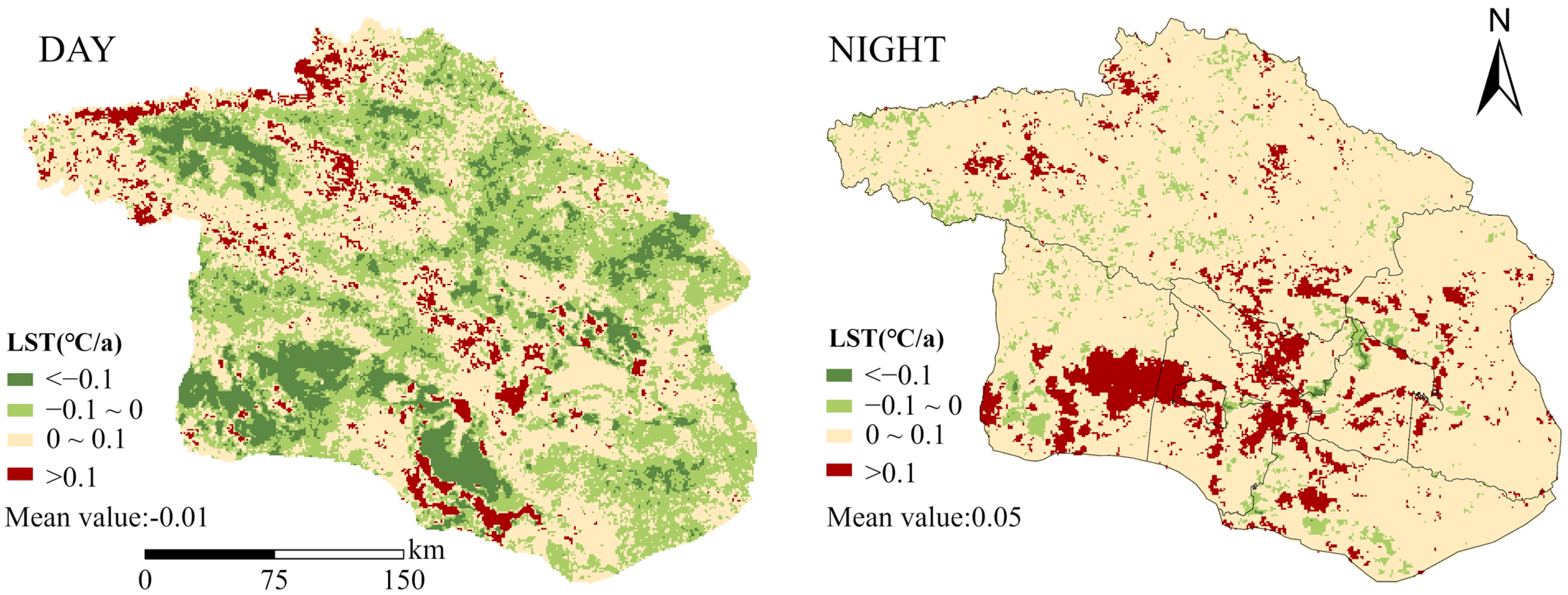
3.3. Characteristics of Land Surface Temperature Change Trends

The change in slope of day/night LST from 2005 to 2020 was obtained using Sen′s slope analysis (Figure 5). The areas with a slope of the annual average daytime surface temperature change greater than 0.1 degrees from 2005 to 2020 are mainly located in the northwestern fringe of the study area, around the Bayinbrook grassland, and in the cultivated land of Kullu and Yuli Counties in the southern part of the study area. At night, the areas with a slope of annual average surface temperature change greater than 0.1 are mainly concentrated in the central part of Rotai County, as well as scattered on the periphery of Bosten Lake. The surface temperature decreases significantly during the day, and the overall LST change rate over 16a is in the range of −1.06~0.70 °C/a. The surface temperature at night shows an overall increasing trend with a change in slope of −0.30~0.36 °C/a, and the change rate is greater during the day than at night.

The results of Sen′s slope analysis were superimposed with the results of the M-K trend test, and the LST change trend levels were obtained based on Table 3. In the results (Figure 6), it can be seen that during the daytime, the areas of highly significantly elevated LST were mainly distributed in and around the Bayinbrook grassland and the northwestern fringe of Hejing County, and there were also large areas of highly significantly elevated areas in the southern part of the study area and in and around Bosten Lake, with highly significantly elevated and significantly elevated areas accounting for 35.72% of the total area. The very significantly lower and significantly lower areas accounted for 2.98% and 9.79% of the total area and were mainly distributed in the peripheral zones of Kullu City and Luntai County. At night, the very significantly elevated and significantly elevated areas were mainly distributed in the eastern region of the study area, concentrated in the eastern regions of Kulle City, Yanqi Hui Autonomous County, and Luntai County, with the very significantly elevated and significantly elevated areas accounting for 38.24% of the total area. Very significantly reduced and significantly reduced areas accounted for 1.52% and 11.59% of the total area and were scattered around Lake Bosten and in the southern fringe of the study area. It is worth noting that the area occupied by non-significantly higher and non-significantly lower is the main type of trend, both during the day and at night.

3.4. Characteristics of Land Surface Temperature Change Trends

In the results of the Hurst index (Figure 7), during the daytime, 63.86% of the areas in the BLB have a continuous future LST trend (Hurst > 0.5), which indicates that the future trend is most likely to be the same as the present one, and another 36.12% of the areas have an unknown future surface temperature trend (Hurst ≤ 0.5). At night, 80.24% of the regional LST trends are persistent in the future (Hurst > 0.5), and 19.76% of the regional LST future trends are unknown (Hurst ≤ 0.5).

To classify the future trend rating of LST, this study superimposed Sen′s slope analysis, the M-K trend test, and the Hurst index to obtain triple information on the trend, significance, and persistence of change (Table 4). In the results (Figure 8), the proportion of the area showing a continuous increase (continuous non-significant increase, continuous significant increase, and continuous highly significant increase) in LST during the daytime is 65.72%, among which the proportion of the area showing continuous significant increase and a continuous highly significant increase is 25.81% and 10.02%, respectively, and is mainly concentrated in the northwestern fringe and central area of Hejing County. Most of the areas around Bosten Lake and Yanqi Hui Autonomous County also showed highly significant elevation, which indicates that LST will further increase in these areas in the future. The future trend of LST was 31.29%, of which 8.06% and 9.74% were continuously and significantly reduced, mainly in the Bayinbrook grassland of Hejing County and the middle and upper regions of Heshuo County, and the rest were scattered in Luntai County and the rest were scattered in the area around Luntai County and Yuli County, indicating that the LST in these areas will maintain a significant decrease in the future.

At night, the future trend of LST is 56.33% in continuously increasing areas, mainly in Kulle City, Heshuo County, Yanqi Hui Autonomous County, Yuli County, and the eastern fringe of Luntai County, and 42.15% in the area continuously decreasing areas, which are mainly scattered around Bosten Lake, the southern fringe of the study area, and a great part of Hejing County. In general, the area of the region where LST continues to rise in the future is larger in both daytime and nighttime, and LST in these regions will maintain a continuously rising trend in the future.

3.5. Analysis of the Drivers of the Spatial and Temporal Distribution of Surface Temperature

3.5.1. Factor Detection Analysis

To investigate the influence of different factors on the diurnal land surface temperature variation in the BLB, 10 detection factors were selected for analysis, the explanatory power q-values of single-factor effects were obtained (

Table 5. Detection results of interannual factors of LST in BLB.

Time	q-Value
	Air Temperature	Precipitation	Altitude	GDP	NPP	Gradient	AOD	NDVI	LULC
2020 day	0.793 *	0.787 *	0.806 *	0.034	0.519 *	0.450 *	0.631 *	0.445 *	0.345 *
2020 night	0.936 *	0.897 *	0.917 *	0.062 *	0.487 *	0.346 *	0.603 *	0.357 *	0.354 *

* Indicates p < 0.01. * Net primary production (NPP); aerosol optical depth (AOD); gross domestic product (GDP); normalized difference vegetation index (NDVI); land-use/land-cover (LULC).

), and the explanatory power of each factor for daytime LST variation was ranked in following order: altitude (0.806) > air temperature (0.793) > precipitation (0.787) > AOD (0.631) > NPP (0.519) > gradient (0.450) > NDVI (0.445) > LULC (0.345) >GDP (0.034). The ranking of the explanatory power of each factor of nighttime LST variation was air temperature (0.936) > altitude (0.917) > precipitation (0.897) > AOD (0.603) > NPP (0.487) > NDVI (0.357) > LULC (0.354) > gradient (0.346) > GDP (0.062), and all factors have p-values less than 0.01, indicating that the explanatory power of all factors is significant. Regardless of day and night, the q-values of elevation and precipitation are greater than 0.3, which are the dominant environmental factors of LST variation in the Bosten Lake basin, while the q-values of GDP are less than 0.3 and have relatively less explanatory power for LST variation in the Bosten Lake basin, thus indicating that natural factors mainly influence LST variation in the BLB.

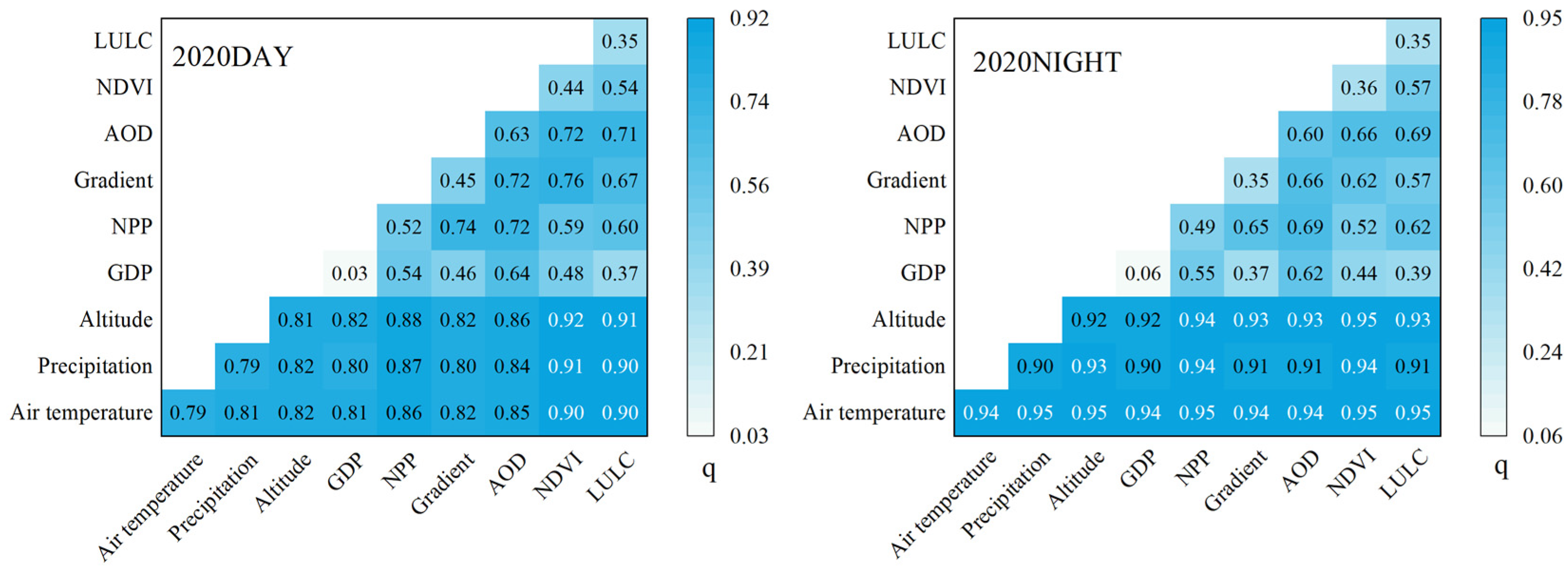
3.5.2. Interaction Detection Analysis

To analyze the extent to which any two factors together explain the change in LST, interaction probes were performed for each factor. The interaction detection results are shown in Figure 9 and the influence after the two-factor interaction is significantly higher than the single factor, and the interaction results of any two factors show a two-factor enhancement or non-linear enhancement, which indicates that the diurnal LST changes in the Bosten Lake basin in 2020 are influenced by the synergy of multiple factors and not controlled by a single factor. During the daytime, the strongest explanatory power was found when the NDVI and elevation were combined, with a q-value of 0.91; at night, the strongest explanatory power was found when NPP and air temperature were combined, with a q-value of 0.95. In summary, the main factors causing diurnal LST changes in 2020 were not homogeneous and differed in the degree of influence on LST changes.

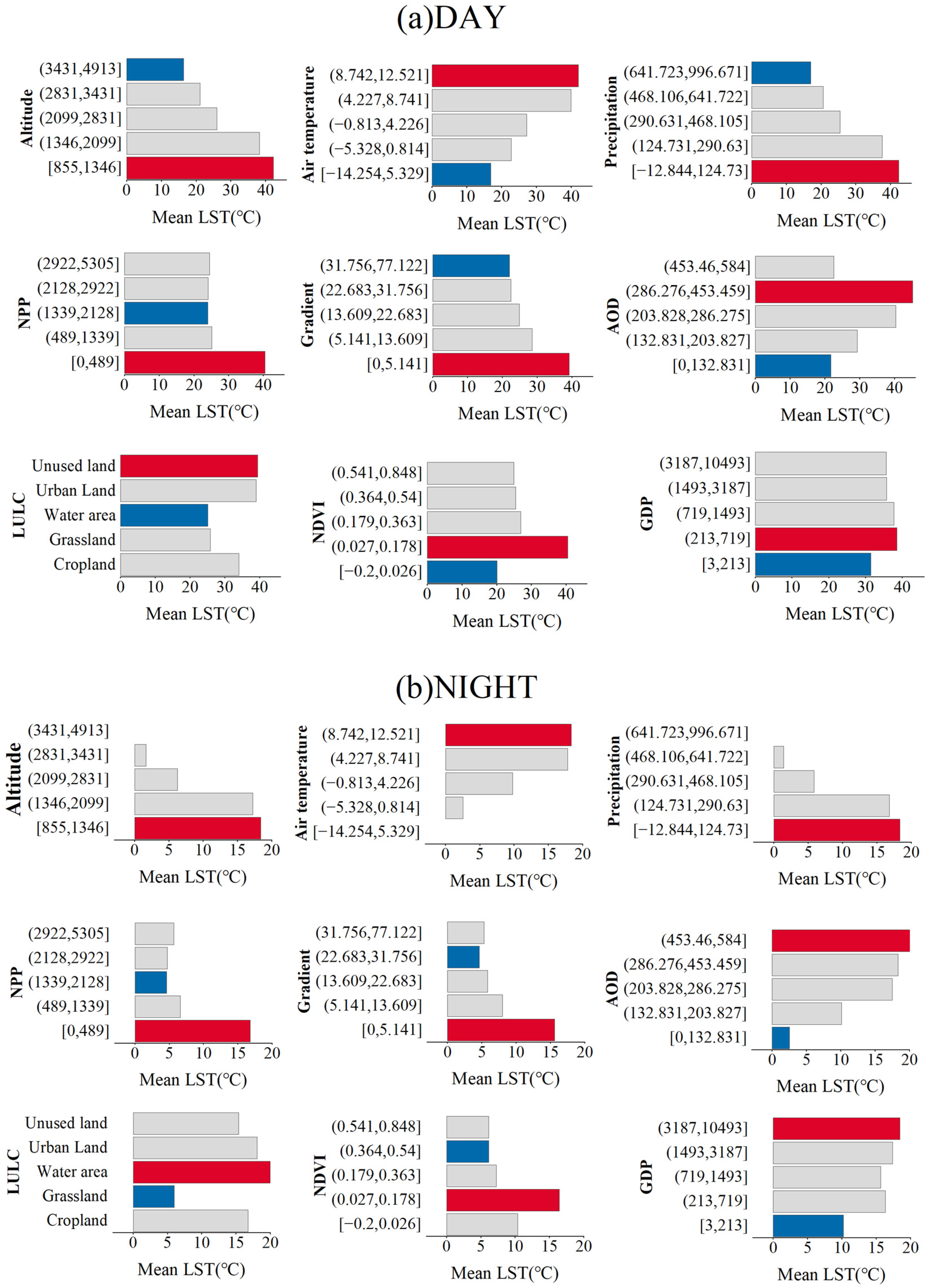
3.5.3. Risk Detection Analysis among Impact Factors

In this study, a risk detector was used to analyze the risk intervals for each influencing factor in the BLB during the day and night. The mean values of LST attributes in the subintervals were at the lowest values for the LST risk intervals of 855–1346 m (elevation), 0–5.141 m (gradient), and −12.844–124.73 mm (precipitation) for altitude, gradient, and precipitation, so LST was negatively correlated with these three dependent variables, while temperature and AOD were positively correlated with LST. From the perspective of LULC, the daytime LULC risk interval occurs in unutilized land, where the high surface temperature is mainly influenced by factors such as solar radiation and the atmospheric greenhouse effect, which make the surface temperature relatively high. The nighttime LULC risk interval occurs in water, where evaporation from the water surface is relatively low at night and the heat of the water body is not easily dissipated, resulting in a relatively high LST (Figure 10).

4. Discussion

4.1. LST Spatiotemporal Distribution and Its Changing Trend

Lake Bosten is located between the desert and the mountains, and the mountainous topographic features lead to the special lake climate of the region [38]. The spatial distribution pattern of LST in the Bosten Lake basin mainly has two typical areas: the first area is the Bayinbruck wetland steppe, and its surrounding mountainous grassland, and the second area is the Bosten Lake and its surrounding oasis. The following analysis will focus on LST change and its formation mechanism in these two areas. During the daytime, the Bayinbruck steppe area located in the northwestern part of the study area shows HT and EHT, and its surrounding mountains show low and very low temperatures; therefore, the Bayinbruck steppe shows the heat island effect, probably because of its many surrounding mountains. The wetland steppe is located in the central basin, the topographic reasons lead to the accumulation of heat, and the high temperature of the basin appears to increase under the influence of the heat gathering effect specific to the topography of the basin [39], which is consistent with the study of [40] on heat gathering in the basin. In contrast, at night, wetland grasslands in the basin show a cold island effect. Some scholars [41] studied relevant studies on wetland cooling, and all indicated that evaporation from wetlands lead to energy loss and cooling of surface water and the cooling effect of wetlands played a role in reducing surface temperature [42]. In the context of global warming, it has been shown that the warming in Asia is mainly due to the increase in LST during the dry season (June–August), and we also found the same trend in the BLB during the dry season, i.e., the mountains and the oasis area in and around Bosten Lake show a continuous warming trend. In addition, the wetland grasslands in the basin show a continuous cooling trend. During the day, Bosten Lake shows a low-temperature state and at night it shows a medium-temperature state, probably because of the large specific heat capacity of the lake water, as the lake absorbs more solar radiation during the day and releases the absorbed heat at night is not prone to extreme temperatures, and has a local climate regulation effect on the oasis area around the lake and the towns (Kullu City, etc.) [43,44]. Other scholars argued this statement when they studied the regulation effect of the lake on the regional climate and stated that the lake can absorb and release a large amount of heat, which plays a certain cooling effect.

4.2. Analysis of LST Influence Factors

Global warming has become one of the major environmental problems facing mankind [45]. We need to determine what factors are causing the increase in surface temperature so that we can improve the environment on which human beings depend. In this study, we found that regardless of diurnal, altitude, precipitation, and temperature are the dominant environmental factors of LST variation in the Bosten Lake basin, which indicates that LST variation is mainly caused by natural factors. Elevation has the greatest effect on the surface temperature of the BLB. The topography of the Bosten Lake basin is complex, with mountains on three sides and many relatively small wetland lakes in the southwest and northwest of Bosten Lake. The Bayinbruck steppe contains many wetlands, many mountain ranges distributed in the region, and large topographic fluctuations, and these complex landscapes together have an important influence on the surface temperature variation in the BLB [46]. The effect of altitude on LST is mainly caused by the air temperature. The higher the altitude, the lower the air temperature and the lower the surface temperature [47,48], which has also been argued in a study of the relationship between altitude and surface temperature, which is consistent with our findings. In addition, lower temperatures, slower vegetation growth at higher altitudes [49], a lower NDVI, and higher surface albedo, results in lower surface temperatures. In contrast, lower altitudes have higher temperatures, vigorous vegetation growth [50], a higher NDVI, and lower surface albedo, which absorbs more energy from solar radiation, resulting in higher surface temperatures [51]. We found that when NPP and air temperature work together, they have a greater effect on surface temperature changes, and there have also been numerous studies on this that show that higher NPP can mitigate the increase in air temperature and provide relief to surface temperature [52]. It works mainly by reducing CO₂ emissions and absorbing the heat released in the process [53].

4.3. Research Limitations and Future Work

In this study, the spatial and temporal distribution pattern of LST, the changing trend, and the influencing factors were explored in the Bosten Lake basin as an example, providing a theoretical basis for the future urban thermal environment as well as sustainable development in the Bosten Lake basin [54], but there are still some limitations. First, this paper only studied the spatial and temporal variation of the diurnal surface temperature in the summer from 2005 to 2020 and did not study the diurnal LST in spring, autumn, and winter seasons, which can be of guidance for ecological environmental protection if future research can be conducted in this area [55]. Secondly, when the influencing factors causing surface temperature were studied, only one factor, GDP, was selected in the selection of socio-economic factors, and influencing factors such as population density and nighttime lighting were considered in the selection of socio-economic factors, but the influence of these factors on the surface temperature was too weak and the influence was not significant, so more influencing factors need to be considered in future studies. Finally, this study only examined the influencing factors using geographic probes, although geographic probes can detect the existence of nonlinear interactions between variables [37], which can overcome the shortcomings of traditional linear regression; however, it may be better to conduct comparative analyses in future studies using random forest regression [56], geographically weighted regression [57], and other methods.

5. Conclusions

Based on MODIS data and supported by GIS spatial analysis technology, this study conducted a quantitative analysis and discussion on the 16-year spatial and temporal variation patterns of LST in the Bosten Lake basin and the influence of different subsurface and impact factors on LST changes, and came to the following conclusions:

(1) The spatial variation characteristics of LST from 2005 to 2020 show that the high-temperature levels are mainly concentrated in Hejing County and the southern region of the study area, regardless of day and night. During the day, the Bayinbruck steppe in Hejing County is the highest LST area and is the main concentration of high and very high temperatures. At night, the LST in the BLB is dominated by very high temperatures and high temperatures, which are mainly distributed in the southern region of Hejing County and the study area, which is exactly opposite to the distribution area of LST levels during the daytime, with significant changes in the spatial pattern of LST. The wetland grasslands in and around the Bayinbruck steppe in the northwestern part of the study area exhibit a heat island effect during the day, while the opposite is true at night. In terms of temporal changes, LST changes in the BLB fluctuate widely, with an overall trend of rising and then falling.

(2) The decreasing trend of LST from 2005 to 2020 is significant during the daytime and vice versa at night, and the change is greater during the daytime than at night. The trend of the diurnal LST is not significant in most regions. In general, the areas where the LST increases and changes significantly are mainly concentrated in Hejing County, Luntai County, and the oasis area around Bosten Lake. In the study of future LST changes, it is found that the changes in LST have the same trend as the present, and it is noteworthy that the areas where future LST increases significantly in day and night have expanded compared with the area occupied by the present, and the overall trend is steadily increasing.

(3) Analysis of spatial and temporal changes in LST using a detector model with a two-factor interaction indicated that the dominant factor of LST changes in 2020 is most strongly explained during the daytime when elevation and the NDVI are combined and at night when NPP and temperature are combined. Regardless of diurnal, altitude, precipitation, and temperature are the dominant environmental factors of LST variation in the BLB. The results from the risk detector show that regardless of day and night, altitude, gradient, and precipitation are negatively correlated with LST, and temperature and AOD are positively correlated with LST. From the perspective of LULC, the daytime LULC risk interval occurs in unutilized land, and the high surface temperature in unutilized land is mainly influenced by factors such as solar radiation and the atmospheric greenhouse effect [58]; unused land receives less precipitation than other land use types which make the surface temperature relatively high. The nighttime LULC risk interval occurs in waters where the evaporation from the water surface is relatively low at night and the heat of the water body is not easily dissipated, making the LST relatively high.

References

1. Deng, Y.; Wang, S.; Bai, X.; Tian, Y.; Wu, L.; Xiao, J.; Chen, F.; Qian, Q. Relationship among Land Surface Temperature and LUCC, NDVI in Typical Karst Area. Sci. Rep. 2018, 8, 1–12. [Google Scholar] [CrossRef] [Green Version]
2. Kikstra, J.S.; Nicholls, Z.R.; Smith, C.J.; Lewis, J.; Lamboll, R.D.; Byers, E.; Sandstad, M.; Meinshausen, M.; Gidden, M.J.; Rogelj, J.; et al. The IPCC Sixth Assessment Report WGIII Climate Assessment of Mitigation Pathways: From Emissions to Global Temperatures. Geosci. Model Dev. 2022, 15, 9075–9109. [Google Scholar] [CrossRef]
3. Zheng, H.; Chen, Y.; Pan, W.; Cai, Y.; Chen, Z. Impact of Land Use/Land Cover Changes on the Thermal Environment in Urbanization: A Case Study of the Natural Wetlands Distribution Area in Minjiang River Estuary, China. Pol. J. Environ. Stud. 2019, 28, 3025–3041. [Google Scholar] [CrossRef]
4. Liang, H.; Kasimu, A.; Ma, H.; Zhao, Y.; Zhang, X.; Wei, B. Exploring the Variations and Influencing Factors of Land Surface Temperature in the Urban Agglomeration on the Northern Slope of the Tianshan Mountains. Sustainability 2022, 14, 10663. [Google Scholar] [CrossRef]
5. Ayanlade, A.; Aigbiremolen, M.I.; Oladosu, O.R. Variations in Urban Land Surface Temperature Intensity over Four Cities in Different Ecological Zones. Sci. Rep. 2021, 11, 20537. [Google Scholar] [CrossRef] [PubMed]
6. Han, B.; Luo, Z.; Liu, Y.; Zhang, T.; Yang, L. Using Local Climate Zones to Investigate Spatio-Temporal Evolution of Thermal Environment at the Urban Regional Level: A Case Study in Xi’an, China. Sustain. Cities Soc. 2022, 76, 103495. [Google Scholar] [CrossRef]
7. Peng, S.-S.; Piao, S.; Zeng, Z.; Ciais, P.; Zhou, L.; Li, L.Z.; Myneni, R.B.; Yin, Y.; Zeng, H. Afforestation in China Cools Local Land Surface Temperature. Proc. Natl. Acad. Sci. USA 2014, 111, 2915–2919. [Google Scholar] [CrossRef] [Green Version]
8. Feldman, A.F.; Short Gianotti, D.J.; Dong, J.; Trigo, I.F.; Salvucci, G.D.; Entekhabi, D. Tropical Surface Temperature Response to Vegetation Cover Changes and the Role of Drylands. Glob. Chang. Biol. 2023, 29, 110–125. [Google Scholar] [CrossRef]
9. Solangi, G.S.; Siyal, A.A.; Siyal, P. Spatiotemporal Dynamics of Land Surface Temperature and Its Impact on the Vegetation. Civ. Eng. J. 2019, 5, 1753–1763. [Google Scholar] [CrossRef]
10. Peng, S.; Piao, S.; Ciais, P.; Friedlingstein, P.; Ottle, C.; Bréon, F.-M.; Nan, H.; Zhou, L.; Myneni, R.B. Surface Urban Heat Island across 419 Global Big Cities. Environ. Sci. Technol. 2012, 46, 696–703. [Google Scholar] [CrossRef]
11. Juhua, L.; Jingcheng, Z.; Wenjiang, H.; Xingang, X.; Ning, J. Preliminary Study on the Relationship between Land Surface Temperature and Occurrence of Yellow Rust in Winter Wheat. Disaster Adv. 2010, 3, 288–292. [Google Scholar]
12. Zhang, F.; Kung, H.; Johnson, V.C.; LaGrone, B.I.; Wang, J. Change Detection of Land Surface Temperature (LST) and Some Related Parameters Using Landsat Image: A Case Study of the Ebinur Lake Watershed, Xinjiang, China. Wetlands 2018, 38, 65–80. [Google Scholar] [CrossRef]
13. Alimujiang, K.; Tang, B.; Gulikezi, T. Analysis of the Spatial-Temporal Dynamic Changes of Urban Expansion in Oasis of Xinjiang Based on RS and GIS. J. Glaciol. Geocryol 2013, 35, 1056–1064. [Google Scholar]
14. Key, J.R.; Collins, J.B.; Fowler, C.; Stone, R.S. High-Latitude Surface Temperature Estimates from Thermal Satellite Data. Remote Sens. Environ. 1997, 61, 302–309. [Google Scholar] [CrossRef]
15. Li, Z.; Duan, S.; Tang, B.; Wu, H.; Ren, H.; Yan, G.; Tang, R.; Leng, P. Review of Methods for Land Surface Temperature Derived from Thermal Infrared Remotely Sensed Data. J. Remote Sens. 2016, 20, 899–920. [Google Scholar]
16. Yue, X.; Li, Z.; Li, H.; Wang, F.; Jin, S. Multi-Temporal Variations in Surface Albedo on Urumqi Glacier No. 1 in Tien Shan, under Arid and Semi-Arid Environment. Remote Sens. 2022, 14, 808. [Google Scholar] [CrossRef]
17. Wang, B.; Ma, Y.; Ma, W. Estimation of Land Surface Temperature Retrieved from EOS/MODIS in Naqu Area over Tibetan Plateau. J. Remote Sens 2012, 16, 1289–1309. [Google Scholar]
18. Jing, S.; Ping, Z.; Qi, Y. A Split-Window Algorithm for Retrieving Land Surface Temperature from ASTER Data. Remote Sens. Technol. Appl. 2012, 27, 728–734. [Google Scholar]
19. Kustas, W.P.; Norman, J.M.; Anderson, M.C.; French, A.N. Estimating Subpixel Surface Temperatures and Energy Fluxes from the Vegetation Index–Radiometric Temperature Relationship. Remote Sens. Environ. 2003, 85, 429–440. [Google Scholar] [CrossRef]
20. Xiong, Y.; Zhao, S.; Yin, J.; Li, C.; Qiu, G. Effects of Evapotranspiration on Regional Land Surface Temperature in an Arid Oasis Based on Thermal Remote Sensing. IEEE Geosci. Remote Sens. Lett. 2016, 13, 1885–1889. [Google Scholar] [CrossRef]
21. Xiao, R.; Weng, Q.; Ouyang, Z.; Li, W.; Schienke, E.W.; Zhang, Z. Land Surface Temperature Variation and Major Factors in Beijing, China. Photogramm. Eng. Remote Sens. 2008, 74, 451–461. [Google Scholar] [CrossRef] [Green Version]
22. Hou, H.; Liu, K.; Li, X.; Chen, S.; Wang, W.; Rong, K. Assessing the Urban Heat Island Variations and Its Influencing Mechanism in Metropolitan Areas of Pearl River Delta, South China. Phys. Chem. Earth Parts A/B/C 2020, 120, 102953. [Google Scholar] [CrossRef]
23. Suo, N.; Yao, Y.; Zhang, B. Comparative Study on the Mountain Elevation Effect of the Tibetan Plateau and the Alps. Geogr. Res 2020, 39, 2568–2580. [Google Scholar]
24. Chen, H.; Liu, L.; Zhang, Z.; Liu, Y.; Tian, H.; Kang, Z.; Wang, T.; Zhang, X. Spatio-Temporal Correlation between Human Activity Intensity and Land Surface Temperature on the North Slope of Tianshan Mountains. J. Geogr. Sci. 2022, 32, 1935–1955. [Google Scholar] [CrossRef]
25. Ahmed, G.; Zan, M.; Kasimu, A. Spatial–Temporal Changes and Influencing Factors of Surface Temperature in Urumqi City Based on Multi-Source Data. Environ. Eng. Sci. 2022, 39, 928–937. [Google Scholar] [CrossRef]
26. Maimaitiyiming, M.; Ghulam, A.; Tiyip, T.; Pla, F.; Latorre-Carmona, P.; Halik, Ü.; Sawut, M.; Caetano, M. Effects of Green Space Spatial Pattern on Land Surface Temperature: Implications for Sustainable Urban Planning and Climate Change Adaptation. ISPRS J. Photogramm. Remote Sens. 2014, 89, 59–66. [Google Scholar] [CrossRef] [Green Version]
27. Jiang, J.; Tian, G. Analysis of the Impact of Land Use/Land Cover Change on Land Surface Temperature with Remote Sensing. Procedia Environ. Sci. 2010, 2, 571–575. [Google Scholar] [CrossRef] [Green Version]
28. Taniguchi, M.; Shimada, J.; Tanaka, T.; Kayane, I.; Sakura, Y.; Shimano, Y.; Dapaah-Siakwan, S.; Kawashima, S. Disturbances of Temperature-Depth Profiles Due to Surface Climate Change and Subsurface Water Flow: 1. An Effect of Linear Increase in Surface Temperature Caused by Global Warming and Urbanization in the Tokyo Metropolitan Area, Japan. Water Resour. Res. 1999, 35, 1507–1517. [Google Scholar] [CrossRef]
29. Wu, Z.; Huang, N.E.; Wallace, J.M.; Smoliak, B.V.; Chen, X. On the Time-Varying Trend in Global-Mean Surface Temperature. Clim. Dyn. 2011, 37, 759–773. [Google Scholar] [CrossRef] [Green Version]
30. Chao, Z.; Wang, L.; Che, M.; Hou, S. Effects of Different Urbanization Levels on Land Surface Temperature Change: Taking Tokyo and Shanghai for Example. Remote Sens. 2020, 12, 2022. [Google Scholar] [CrossRef]
31. Wang, H.; Pan, Y.; Chen, Y. Impacts of Regional Climate and Teleconnection on Hydrological Change in the Bosten Lake Basin, Arid Region of Northwestern China. J. Water Clim. Chang. 2018, 9, 74–88. [Google Scholar] [CrossRef]
32. Zhao, W.; Duan, S.-B. Reconstruction of Daytime Land Surface Temperatures under Cloud-Covered Conditions Using Integrated MODIS/Terra Land Products and MSG Geostationary Satellite Data. Remote Sens. Environ. 2020, 247, 111931. [Google Scholar] [CrossRef]
33. Wang, Y.; Yao, Y.; Chen, S.; Ni, Z.; Xia, B. Spatiotemporal Evolution of Urban Development and Surface Urban Heat Island in Guangdong-Hong Kong-Macau Greater Bay Area of China from 2013 to 2019. Resour. Conserv. Recycl. 2022, 179, 106063. [Google Scholar] [CrossRef]
34. Yu, H.; Bian, Z.; Mu, S.; Yuan, J.; Chen, F. Effects of Climate Change on Land Cover Change and Vegetation Dynamics in Xinjiang, China. Int. J. Environ. Res. Public Health 2020, 17, 4865. [Google Scholar] [CrossRef]
35. Hamed, K.H. Trend Detection in Hydrologic Data: The Mann–Kendall Trend Test under the Scaling Hypothesis. J. Hydrol. 2008, 349, 350–363. [Google Scholar] [CrossRef]
36. Jiang, T.-H.; Deng, L.-T. Some Problems in Estimating a Hurst Exponent-a Case Study of Applicatings to Climatic Change. Sci. Geogr. Sin. 2004, 24, 177–182. [Google Scholar]
37. Wang, J.; Xu, C. Geodetector: Principle and Prospective. Acta Geogr. Sin. 2017, 72, 116–134. [Google Scholar]
38. Masson-Delmotte, V.; Zhai, P.; Pörtner, H.-O.; Roberts, D.; Skea, J.; Shukla, P.R.; Pirani, A.; Moufouma-Okia, W.; Péan, C.; Pidcock, R.; et al. Global Warming of 1.5 C. IPCC Spec. Rep. Impacts Glob. Warm. 2018, 1, 43–50. [Google Scholar]
39. Yu, H.; Zhang, H.; Yang, Y. An Analysis of Extremely Hot Weather Process on Turpan Basin. Clim. Chang. Res. Lett. 2013, 2, 109–113. [Google Scholar] [CrossRef]
40. Lin, W.; Wang, G.; Zhang, S.; Zhao, Z.; Xing, L.; Gan, H.; Tan, X. Heat Aggregation Mechanisms of Hot Dry Rocks Resources in the Gonghe Basin, Northeastern Tibetan Plateau. Acta Geol. Sin.-Engl. Ed. 2021, 95, 1793–1804. [Google Scholar] [CrossRef]
41. Sun, R.; Chen, A.; Chen, L.; Lü, Y. Cooling Effects of Wetlands in an Urban Region: The Case of Beijing. Ecol. Indic. 2012, 20, 57–64. [Google Scholar] [CrossRef]
42. Li, Z.; Liu, X.; Ma, T.; Kejia, D.; Zhou, Q.; Yao, B.; Niu, T. Retrieval of the Surface Evapotranspiration Patterns in the Alpine Grassland–Wetland Ecosystem Applying SEBAL Model in the Source Region of the Yellow River, China. Ecol. Model. 2013, 270, 64–75. [Google Scholar] [CrossRef]
43. Tranvik, L.J.; Downing, J.A.; Cotner, J.B.; Loiselle, S.A.; Striegl, R.G.; Ballatore, T.J.; Dillon, P.; Finlay, K.; Fortino, K.; Knoll, L.B.; et al. Lakes and Reservoirs as Regulators of Carbon Cycling and Climate. Limnol. Oceanogr. 2009, 54, 2298–2314. [Google Scholar] [CrossRef] [Green Version]
44. Shimoda, Y.; Azim, M.E.; Perhar, G.; Ramin, M.; Kenney, M.A.; Sadraddini, S.; Gudimov, A.; Arhonditsis, G.B. Our Current Understanding of Lake Ecosystem Response to Climate Change: What Have We Really Learned from the North Temperate Deep Lakes? J. Great Lakes Res. 2011, 37, 173–193. [Google Scholar] [CrossRef]
45. Hoegh-Guldberg, O.; Jacob, D.; Bindi, M.; Brown, S.; Camilloni, I.; Diedhiou, A.; Djalante, R.; Ebi, K.; Engelbrecht, F.; Guiot, J.; et al. Impacts of 1.5 C Global Warming on Natural and Human Systems. Glob. Warm. 1.5 °C 2018. [Google Scholar]
46. Li, X.; Zhang, F.; Chan, N.W.; Shi, J.; Liu, C.; Chen, D. High Precision Extraction of Surface Water from Complex Terrain in Bosten Lake Basin Based on Water Index and Slope Mask Data. Water 2022, 14, 2809. [Google Scholar] [CrossRef]
47. Peng, X.; Wu, W.; Zheng, Y.; Sun, J.; Hu, T.; Wang, P. Correlation Analysis of Land Surface Temperature and Topographic Elements in Hangzhou, China. Sci. Rep. 2020, 10, 10451. [Google Scholar] [CrossRef]
48. Özhancı, E.; Koç, A. The Effect of Different Area Uses and Topography on Surface Temperature and Climate Parameters. Environ. Sci. Pollut. Res. 2023, 30, 47038–47051. [Google Scholar] [CrossRef]
49. Xu, H.; Li, T.-B.; Chen, J.-N.; Liu, C.-N.; Zhou, X.; Xia, L. Characteristics and Applications of Ecological Soil Substrate for Rocky Slope Vegetation in Cold and High-Altitude Areas. Sci. Total Environ. 2017, 609, 446–455. [Google Scholar] [CrossRef]
50. Marston, R.A.; Anderson, J.E. Watersheds and Vegetation of the Greater Yellowstone Ecosystem. Conserv. Biol. 1991, 5, 338–346. [Google Scholar] [CrossRef]
51. Marzban, F.; Sodoudi, S.; Preusker, R. The Influence of Land-Cover Type on the Relationship between NDVI–LST and LST-T Air. Int. J. Remote Sens. 2018, 39, 1377–1398. [Google Scholar] [CrossRef]
52. Lu, X.-Y.; Chen, X.; Zhao, X.-L.; Lv, D.-J.; Zhang, Y. Assessing the Impact of Land Surface Temperature on Urban Net Primary Productivity Increment Based on Geographically Weighted Regression Model. Sci. Rep. 2021, 11, 22282. [Google Scholar] [CrossRef]
53. Mao, D.; Luo, L.; Wang, Z.; Zhang, C.; Ren, C. Variations in Net Primary Productivity and Its Relationships with Warming Climate in the Permafrost Zone of the Tibetan Plateau. J. Geogr. Sci. 2015, 25, 967–977. [Google Scholar] [CrossRef] [Green Version]
54. Wang, Y.; Zhang, S.; Chang, X. Evapotranspiration Estimation Based on Remote Sensing and the SEBAL Model in the Bosten Lake Basin of China. Sustainability 2020, 12, 7293. [Google Scholar] [CrossRef]
55. Peng, J.; Xie, P.; Liu, Y.; Ma, J. Urban Thermal Environment Dynamics and Associated Landscape Pattern Factors: A Case Study in the Beijing Metropolitan Region. Remote Sens. Environ. 2016, 173, 145–155. [Google Scholar] [CrossRef]
56. Grömping, U. Variable Importance Assessment in Regression: Linear Regression versus Random Forest. Am. Stat. 2009, 63, 308–319. [Google Scholar] [CrossRef]
57. Brunsdon, C.; Fotheringham, S.; Charlton, M. Geographically Weighted Regression. J. R. Stat. Soc. Ser. D (Stat.) 1998, 47, 431–443. [Google Scholar] [CrossRef]
58. Kondratyev, K.Y.; Varotsos, C. Atmospheric Greenhouse Effect in the Context of Global Climate Change. Il Nuovo Cim. C 1995, 18, 123–151. [Google Scholar] [CrossRef]
Figure 1. Location map of the study area.
Land 12 01185 g001
Figure 2. Research framework diagram.
Land 12 01185 g002
Figure 3. Space distribution map of LST class in the BLB.
Land 12 01185 g003
Figure 4. Diurnal variation of LST in the BLB.
Land 12 01185 g004
Figure 5. Spatial distribution of slope in the BLB from 2005 to 2020.
Land 12 01185 g005
Figure 6. The changing trend of LST in the BLB from 2005 to 2020.
Land 12 01185 g006
Figure 7. Spatial distribution map of the Hurst index in the BLB from 2005 to 2020.
Land 12 01185 g007
Figure 8. Future trends of LST in the BLB. (Nsc means no significant change; Chsr means continued highly significant reduction; Csr means continued significant reduction; Snsd means sustained non-significant decrease; Snse means sustained non-significant elevation; Cse means continued significant elevation; Chse means continued highly significant elevation.)
Land 12 01185 g008
Figure 9. The 2020 diurnal BLB interaction detection results.
Land 12 01185 g009
Figure 10. The risk interval or category of each influencing factor in the daytime and nighttime. Note: red indicates the highest average LST in the interval and blue indicates the lowest.
Land 12 01185 g010