
Urban Development and Transportation: Investigating Spatial Performance Indicators of 12 European Union Coastal Regions


School of Rural & Surveying Engineering, Aristotle University of Thessaloniki, 54124 Thessaloniki, Greece
*
Author to whom correspondence should be addressed.
Land 2023, 12(9), 1757; https://doi.org/10.3390/land12091757
Submission received: 10 August 2023
/
Revised: 1 September 2023
/
Accepted: 6 September 2023
/
Published: 10 September 2023
(This article belongs to the Special Issue Land Use Planning for Post COVID-19 Urban Transport Transformations)
Abstract
:Urbanization is one of the most dominant economic and social changes of the 20th century. This phenomenon brings about rapid urban development, which is inextricably linked to transport development. In order to understand this relationship, it is important to analyze the spatial spillover effects of the phenomenon in the urban environment. This study analyzes the spatial performance, in terms of urban development, of 12 European Union regions from five European countries with coastal areas by incorporating spatial data such as length of road network, population distribution, land uses, and other factors. Key performance indicators have been developed for evaluating the structural development model of the regions (e.g., dense or sprawl development). In addition, the incorporation of spatial spillover effects in the evaluation of the regions was conducted by the extended spatial data envelopment analysis (SDEA) method. The results of SDEA identified the best and worst-performing regions in terms of urban growth. Finally, this study implements a target-setting approach where under-performing regions can best perform. Based on the target-setting approach, local authorities can set realistic targets for improving the structural model that the regions are following.
1. Introduction
While population growth in 2021 in the European Union (EU) showed a decrement (10% compared to 2020), urbanization continued to increase, adding more than half a million people to the urban population compared to the years 2021 and 2020 [1]. Thus, the trend towards urbanization is expected to continue in the coming years, and by 2050, the urban population is predicted to be twice today’s numbers, where 7 out of 10 people live in cities [2]. However, the speed and scale of the urbanization phenomenon create challenges in different areas, one of which is the well-connected transport system [3].
Undoubtedly, transport plays an important role in the pace of urbanization and urban growth. The study by Aljoufie et al. (2013) [4] revealed that transport infrastructure is a constantly strong spatial influencing factor in urban growth. Transportation systems provide essential choices for the movement of both people and goods and influence development patterns and levels of economic activity through the accessibility they provide to space [5]. Thus, urban development (urbanization) and transport are inextricably linked. According to [6], developments in transport infrastructure result in urban development and even land use change. Respectively, urban development affects transportation; for example, it increases demand time [7,8,9] but also causes traffic congestion [10,11].
On the one hand, transport infrastructure (e.g., roads) attracts urban growth, but on the other hand, residential growth and population increase the demand for travel and therefore increase the need for more transport infrastructure. Therefore, understanding the interaction between urban development and transport is essential in the field of transport, as it can help create strategies related to urban development. For instance, Ref. [12] reviewed and presented the scenario-based planning methods applied for studying the effects of transportation on urbanization.
Analyses of urban development should also take into consideration the spatial performances of cities and the spatial interconnections between different cities. Zhang et al. (2022) [13] have studied the performance of a polycentric space formation and tested the spatial performance of cities. An additional application of spatial analysis was implemented by Wang and Zhou (2022) [14], where they analyzed the spatial pattern of urban and rural community differentiation and evaluated spatial differences in the level of accessibility to four types of public service facilities based on the shortest travel distance.
The analysis of the urban development of cities has been applied in several studies, as presented above, with many of them focusing on transportation. An additional factor that affects urban development but is highly related to the transport infrastructure is tourism, which is mostly observed in cities with airports and ports. Ji and Wang (2022) [15] studied the role of tourism in the economic development of 39 coastal cities in China from 2010 to 2019 using the entropy method, the Dagum Gini coefficient, kernel density estimation, and the spatial Durbin model. Doerr et al. (2020) [16] estimated the effects of new airport infrastructure on arrivals of tourists in the Bavarian region of Allagau and presented that additional tourist inflows are particularly well observed in the country where the airport is located. Furthermore, Boulos (2015) [17] presented that constructing services that are required for the port by the city keeps the balance between port and city growth. Therefore, studying the urban development of the European Union (EU) regions seems to be ideal for understanding how these regions are affected by neighboring regions, even from different countries, and how transport infrastructure, demographic context, and landscape (coastline) are affecting urban growth. It is even more interesting to investigate regions with coastal areas since these regions are facing difficulties in terms of planning due to the limited and extremely expensive land areas along the coast [18].
Studying the urban structure of the regions in relation to other factors alongside transportation will provide an essential overview of the phenomenon and identification of whether sustainable cities are more efficiently operating. For instance, improving cycling infrastructure may help avoid barriers to cycling, which must be on the planning developers’ agenda [19]. The same objective stands also for the case of walkability, which should be analyzed, such as in the work of Amprasi et al. (2020) [20]. Additionally, the effects of public transport on urban growth are essential (e.g., [21]).
Therefore, this study is developed to study the spatial spillover effects of urban development in relation to transportation and demographic context over 12 EU coastal regions from five different countries. These regions are namely: Bouches-du-Rhone (France); Alpes-Maritimes (France); Herault (France); Attiki (Greece); Central Macedonia (Greece); Larnaca (Cyprus); Limassol (Cyprus); Bari (Italy); Napoli (Italy); Genova (Italy); Barcelona (Spain) and Valencia (Spain). These coastal regions were selected due to the fact that they cover a wide area of the European region and they at least have one airport or/and one port infrastructure, which denotes the direct and indirect interconnection that they might have. Moreover, the selection of several coastal areas from different administrative and landscape settings (coastline) will reveal significant insights into spatial interrelationships between the areas, similarities or dissimilarities in spatial patterns, and the spatial performance of the regions.
For developing spatial models, there is a constraint on obtaining multitemporal data over at least three time frames that generate a cohesive vision that may be validated for future urban outcomes [22]. Additionally, the availability of spatiotemporal data at a regional level is limited, which has generated limitations on the availability of methodological approaches for analyzing the spatial pattern of this phenomenon.
Another trustworthy preliminary approach for analyzing the spatial relationship between urban development and transportation systems is the development of indicators (e.g., [23]). For example, Aljoufie et al. (2012) [24] developed several indicators that revealed the relationship between urban growth and transportation. Boeing et al. (2022) [25] produced comparative spatial indicators for benchmarking 25 diverse cities in terms of urban design and transport features, which are considered important for public health and sustainability. Dur and Yigitcanlar (2015) [26] developed an indicator-based spatial composite indexing model for measuring the sustainability performance of urban settings by considering land-use and transport integration principles. Another study on spatial analysis was conducted by Dur et al. (2014) [27], where they integrated land use and the transportation system at a neighboring level.
Besides the indication of the spatial patterns that the indices will reveal for all the 12 EU regions, the indices are not directly able to identify and quantify adequately the spatial performance of the areas, and thus this study implemented a spatial benchmarking approach for measuring the efficiency of each region in terms of their urban development performance in relation to their transportation, demographic and land use growth. A trustworthy benchmarking method for evaluating performance is data envelopment analysis (DEA), which is widely used, such as in the fields of freight transportation (e.g., [28]). For instance, Olejnik et al. (2021) [29] introduced a modification of the CCR DEA method by extending the method to its spatial form, including spatial interactions and creating the spatial data envelopment analysis (SDEA) method. Moreover, Desai and Storbeck (1990) [30] proposed a DEA framework for measuring the relative spatial efficiency of locational decisions.
The results of this analysis revealed significant findings about the regions’ performance in terms of their urban development. Key performance indicators (KPIs) revealed, for example, that Limassol is a denser region compared to Napoli, which seems to follow a sprawling structural model. Additionally, the results of the SDEA revealed which regions performed best and under-perform in terms of urban development. Limassol again appeared to best-perform the indication of population density, which showed Limassol as one of the best-performing regions. In addition to the SDEA method, a target-setting approach was implemented for estimating the extent of improvement that every under-performing region should reach in order to perform at its best.
2. Methodological Framework
In order to better understand the methodological framework that was approached in this study, the following flowchart was developed, presenting all the steps followed (Figure 1). Based on the flowchart, the first step was the elaboration of the collected shapefiles concerning the 12 coastal regions for obtaining information about the regions (e.g., demographic context) and thus the creation of the database.
Based on the collected data, some of the information was used for creating the KPIs, which were used for evaluating the current urban development status of the regions. Furthermore, each KPI was developed to capture the urban development of the regions. For instance, some KPIs were developed for evaluating the development of the regions in terms of transportation. Moreover, the use of the KPIs provided a ranking of the regions based on their values (performance) corresponding to each different KPI. The ranking of the regions revealed how diverse, in terms of urban development, the EU coastal regions are, which can be used by local authorities in order to observe if their region is under- or best-performing compared to the other regions of the same country and also the factors that make their region under-perform.
Additionally, the fact that KPIs can capture the urban development performance of the regions is still an inadequate method for providing comparative evaluations and considering the input factors of the regions. DEA is a benchmarking method that provides an adequate evaluation of the under-investigation regions. However, since the urban spatial growth of the regions is being investigated, it was considered essential to incorporate the spatial spillover effects that may exist between the regions in terms of urban growth. For validating this spatial dependence between the regions, Moran’s I Test was implemented, considering each different KPI as an output.
In cases where spatial dependence exists, the SDEA method is implemented, incorporating the spatial spillover effects in the evaluation process. As in DEA, SDEA can identify best- and under-performing regions based on their inputs and outputs. Furthermore, one additional application of SDEA is the target-setting process, where targeted values of the outputs can be estimated for the under-performing regions by taking as benchmarks the best-performing regions.
2.1. Morans’ I Test
A classic measure of spatial autocorrelation is the Moran’s I Test, which is widely used in different research, e.g., [31]. Moran’s I Test is a measure of autocorrelation that compares the data from neighboring units (e.g., EU regions), as denoted by a spatial weight matrix and identifies the existence of a spatial dependence between the units, following the below equation:
where, and are the deviation of an attribute for feature and , respectively, from its mean , is the spatial weight matrix between the units and , is equal to the total number of units and is the aggregate of all the spatial weights.
The p-value computed in Moran’s I Test clarifies the assumption of spatial dependence. In detail, if the p-value is significant (p-value ≤ 0.05), then the null hypothesis is rejected, which means that spatial dependence exists.
2.2. Benchmarking Analysis
Benchmarking analysis is an evaluation of performance that compares different under-study units (i.e., the 12 coastal regions) and provides efficient outputs of how efficiently a unit is performing on different subjects. One way to make rational, ideal evaluations is by setting key performance indicators (KPIs) [32]. These are numbers or percentages that reflect the phenomenon (e.g., scale of urbanization, sprawl phenomena, etc.). Besides the adequate overall “picture” that KPIs provide about the performance of each unit, they cannot capture the spatial spillover effects that affect the phenomenon of urban growth.
A classic benchmarking method that can incorporate explanatory variables with the dependent variable and provide an efficient rate of the units’ performance is DEA, which was developed by Charnes et al. (1978) [33]. DEA is a very powerful service management and benchmarking technique [34]. Equation (2) presents the formation of an output-oriented DEA method:
Subject to:
where
= the number of units being compared in the DEA analysis
= efficiency rating of the service unit being evaluated by the output-oriented DEA model
= amount of output r used by unit j
= amount of input i used by unit j
= number of inputs
= number of outputs
= coefficient or weight assigned by the DEA to output r
= coefficient or weight assigned by the DEA to input i
Output-oriented DEA models attempt to maximize the outputs by using the same inputs, while the input-oriented DEA model’s objective is to minimize the inputs while keeping the same outputs. The maximization of θ indicates the maximization of the output variable in the DEA output-oriented model, which will provide the efficiency scores of the regions. A solution of the output-oriented model can also be obtained from the solution of the input-oriented model, as presented in Equation (3) [35]:
where
= efficiency rating of the service unit being evaluated by the input-oriented DEA model
The efficiency scores of the input-oriented model are between 0 and 1, where units with efficiency scores equal to 1 are efficient and units with values below 1 are considered inefficient. Therefore, based on Equation (3), the efficiency scores obtained from the maximization of Equation (2) obtain values equal to 1 and above 1, where values equal to 1 indicate best-performing regions (efficient) and values above 1 indicate under-performing regions (inefficient).
To incorporate the spatial spillover effects that may exist, this study develops a SDEA model that incorporates the spatial interrelation between the EU regions, considering the spatial spillover effects that urbanization has on the cities’ structure. Equation (4) presents the SDEA model formation:
Subject to:
where
= is the spatial weight matrix representing the spatial connection of unit with unit . The diagonal of the matrix is zero.
There are several criteria for estimating the spatial weight matrix, such as the Rook’s criterion, Queen’s criterion, k-nearest neighbors criterion, distance-based criterion, etc. Rook’s criterion defines the neighbors by the existence of a common edge between two regions. The Queen’s criterion defines neighbors as units sharing a common edge or vertex. In this study, the 12 EU regions are not spatial neighbors, except for the regions of Larnaca and Limassol in Cyprus. Therefore, if the Rook’s and Queen’s criteria are used for the design of the weight matrix, all the regions, except for Larnaca and Limassol, will appear to have a zero spatial connection with any of the other regions.
The distance-based criterion, which was used in this study for the weight matrix formation, defines the distance between the regions using the Euclidean distance equation (Equation (5)). The distance between the regions is measured from the centroid of each region.
Equation (6) presents the formation of the connectivity matrix between the different regions. The hypothesis developed in the connectivity matrix is that every region is connected with every other region with multimodality (roadway, airway and waterway).
The weights in the matrix define the weight of connectivity between the regions and , which is denoted in Equation (7).
Therefore, in this study, the spatial weight matrix developed was based on the distance-based criterion. The k number of nearest neighbors was 11, meaning that every region is connected with the other 11 regions of this study (all regions are spatially connected between them). The reason for investigating this criterion with k = 11 was to observe how the spatial connection that these regions may share is affecting their performance. The connectivity matrix also represented the spatial connection these areas have through multimodality (waterways, airways and roadways). Figure 2 presents the 12 EU regions that where uincluded in this study.
2.3. Target Setting Approach
This section presents the mathematical formulation of the target-setting process. In detail, by using Equation (7), under-performing regions, in terms of spatial urban growth, will be used for calculating their targeted outputs (KPIs) that they should have in order to best-perform, i.e., an efficiency score equal to 1, having the same input values and by considering the best-performing regions as benchmarks. Therefore, this process can support the efforts of policymakers and local authorities to the extent of improvement in terms of urban development. For example, if two of the twelve regions best-perform (efficiency score equals to 1) for one specific KPI, then these regions will be used as benchmarks for the other 10 under-performing regions (efficiency score > 1) and thus their targeted value for the specific KPI will be estimated (using Equation (8)), considering that their inputs remain constant. More simply, the target-setting approach estimates the value of the output (KPI) that every under-performing region should have, given the same inputs and by following the best-performing regions.
where
= targeted value for the under-performing region
= lambda weight corresponding to the benchmarking regions
= KPI in the benchmarking region
3. Study Area and Data Sources
3.1. Research Scope and Study Areas
The research scope of this study is the evaluation of the existing urban growth of 12 EU regions from five European Union countries in relation to the spatial spillover effects that exist between the regions. These regions are in coastal areas and have a significant effect on the urban structure of the regions due to the increased phenomenon of tourist visits (i.e., financial enhancements in these areas from tourists’ expenses) and the limitation of the coastline, which might be considered as urban development “barriers” that sometimes prevent urban planners from promoting a uniform urban expansion of the regions. To study the spatial structure of the regions, several spatial performance indices were developed based only on open-source information. Therefore, this paper analyzes the efficiency of the regions in terms of urban development, considering their transport infrastructure, land uses, and demographic context and finally incorporating possible spatial spillover effects between the regions. Furthermore, identified under-performing regions were addressed by proposing target values in terms of development in order to best-perform.
3.2. Data and Key Performance Indicators
Analyzing the urban development of a region requires the collection of spatial and temporal data. However, due to the lack of bidimensional data (space and time) many of the analyses were developed to analyze only the spatial or temporal dimensions of the phenomenon.
This study was developed by collecting geoinformation concerning 12 coastal regions from five EU countries, namely: Bouches-du-Rhone (France); Alpes-Maritimes (France); Herault (France); Attiki (Greece); Central Macedonia (Greece); Larnaca (Cyprus); Limassol (Cyprus); Bari (Italy); Napoli (Italy); Genova (Italy); Barcelona (Spain) and Valencia (Spain). The criteria for selecting these regions were: coverage of a wide area of the Mediterranean Sea (from west to east); the fact that they at least have one airport or/and one port; and the availability of data.
Table 1 presents the geoinformation collected from different sources but also the data that occurred from the elaboration of the primarily collected data (e.g., length of road network, number of buildings, etc.) As can be seen from the table, the collected data provides information on different contexts of the regions, such as transportation (road, cycleway, pedestrian and public transport infrastructure) and demographic (population).
The spillover effects of urbanization and unorthodox urban development have created a complex urban structure for the regions that affect transportation and vice versa. Thus, for the evaluation and identification of the regions’ spatial performance, key performance indicators (KPIs) were developed. The KPIs were developed based on the combinations of the data from Table 1 and are presented in Table 2.
The results of the implementation of the above nine KPIs are presented in the next section. Each of the above indicators expresses different aspects of the structural performance of the EU regions. Implementing these KPIs will reveal insights into the performance of each region compared to the others and will assist in the process of identifying which regions are affected by the phenomenon of urbanization. Furthermore, the urban development of the regions can be essentially affected by the transportation network (e.g., the public transport network), and thus the KPIs also provide an overview of this effect.
Prior to the implementation of the SDEA method, a correlation analysis was implemented to observe which noncollinear data would be used as inputs in the model. Figure 3 presents the concluded dataset that was used in the SDEA method, which, as can be seen, includes noncollinear variables. Some findings that can be discussed from this figure are that the coastline length of the regions is strongly, but not collinearly (collinear coefficient > 0.7), related to the public transport infrastructure, the number of parking locations, the industrial area and the residential area. This observation indicates that the coastline is indeed related to transport (e.g., public transport infrastructure) and to the region’s land use (e.g., residential and industrial areas). Regarding the correlation between the coastline and industrial use, the significant correlation value can be justified by the fact that the regions that were analyzed in this study have industrial ports, which cover a significant proportion of their coastline length. Additionally, it seems that industrial areas are also correlated to parking locations and residential areas, which might indicate that urbanization is increasing in areas where job positions exist (e.g., industrial areas). As for the public transport variable, it seems that it is correlated with residential areas, commercial areas, the number of POIs, parking locations and industrial areas, so it is expected to observe an increased public network in residential and commercial areas where parking locations and an increased number of POIs exist. Another significant observation from the correlation analysis is that larger regions (province areas) have larger residential and industrial areas, which is also an indication of urbanization.
The following section will present the outcomes that occurred from this study’s analysis for a better overview of the urban growth in each coastal region.
4. Results
This section presents the results obtained by implementing the above methodological framework. Figure 4 presents the current urban structure of the regions alongside their density index. As can be observed from the figure, some of the regions are developed mainly along their coastlines (e.g., Valencia). However, there are also some regions that follow a mixed spatial development, i.e., along the coastline and inland spatial development (e.g., Bari, which presents both spatial development structures). Besides the indication of the population density inside the regions, the figure below does not offer detailed information on how the regions are spatially developed.
4.1. Key Performance Indicators
This section presents the overall results obtained from the KPI evaluation, as denoted in Table 3. The table below revealed heterogeneity in terms of spatial urban growth between regions from the same country in some KPIs. For instance, in KPIs 1 and 2, Larnaca and Limassol, both regions in Cyprus, appeared to be heterogeneous, which indicates that even for closed regions (in terms of distance), regions that follow the same development policies with approximately the same spatial characteristics seem to perform differently. The following subsections describe each KPI separately, providing a detailed “picture” of the regions’ performances in terms of their spatial urban growth. The ranking of the regions is also presented, which can be used by local authorities to observe the performance of their region and to be able to identify the best-performing regions in the same country that are possibly following the same policies but performing differently.
4.1.1. KPI 1: Buildings’ Capacity
This KPI expresses the building’s capacity, i.e., how many people correspond to each square meter. Thus, larger values of this KPI indicate that the structure of the city is dense rather than spreading. In detail, the building’s area (square meters) in residential zones indicates the area that the buildings cover in residential land. Based on this KPI, Limassol seems to be a dense region where each square meter corresponds to seven people. Genova and Barcelona are following Limassol in this indicator, with Hérault being the last region in ranking, which can be interpreted as meaning that these regions have larger buildings than their respective populations.
4.1.2. KPI 2: Population Density
This measure provides a value that represents the number of people per square meter of residential land. Additionally, this measure is a good indication of how much residential land exists compared to the population, i.e., higher values of this KPI indicate that an area is denser compared with regions with lower values of the same KPI. This indication can also be used by planners while following strategies such as extending the boundaries of the residential zones, which will lead to the sprawling structure of the regions. Limassol appears to be an example case in this KPI, followed by Genova, Bari and Napoli. The last-ranking regions in terms of this KPI are Larnaca, Alpes-Maritimes and Hérault. Moreover, it is worth mentioning that the heterogeneity between the regions of the same country, e.g., Larnaca and Limassol, which raises speculation that these regions, even from the same country, may have a different planning strategy. However, this cannot be validated, but it can be captured in the SDEA method, where closer areas show a higher spatial spillover effect and thus an effect on their urban growth performance.
4.1.3. KPI 3: Building’s Coverage
Building’s coverage KPI provides a value of the covered residential land area from buildings and is expressed as a percentage. Lower values indicate that the buildings have not covered the existing available residential land area. Therefore, higher values of this KPI can be interpreted as follows: that buildings have covered most of the existing residential land area and thus planners should focus on extending this area to fulfill the urban growth (type of sprawl region) or that smaller residential land areas are covered by buildings (type of dense region). The regions with the lowest values of this KPI are Limassol, Larnaca and Central Macedonia. The interpretation of this KPI should be combined with the intel of KPI 2 and the following KPI.
Thus, the information from this KPI should be combined with the information from KPI 2. Smaller percentages of KPI 3 and higher values of KPI 2 (e.g., Limassol) indicate a dense region, in contrast to higher percentages of KPI 3 and smaller values of KPI 2 (e.g., Napoli, Hérault), which indicate a sprawling region.
4.1.4. KPI 4: Residential Area Coverage
This KPI measures the residential area compared to the total area of the region, expressed as a percentage. Therefore, based on this KPI, the requested percentages should be low because a high percentage indicates that regions are following a sprawl model of urban development. However, to conclude with a robust “picture” of which type of urban growth (sprawl or dense) the regions are following, the information from this KPI, along with KPI 3 and KPI 2, is combined.
For example, Napoli has the highest percentage of residential land in the total region’s area (KPI 4), the highest percentage of covered residential land by buildings (KPI 3) and one of the lowest values of population per residential land area (KPI 2), which leads to the conclusion that Napoli follows a sprawl model of urban development. On the other side, Limassol and Barcelona have lower percentages in KPI 3 and KPI 4 and larger values in KPI 2, which indicates a dense model of urban development. Combining this information with the correlation analysis, it seems that the coastline has an affection for the model structure, since residential areas are positively affected by the length of the coastline. In detail, as the coastline increases, the residential land area also increases. However, this increment leads to a respective increase in KPI 4 and a decrease in KPIs 2 and 3. The same interpretation can be applied to the rest of the regions.
4.1.5. KPI 5: Commercial Area Coverage
This KPI identifies the economic growth of the areas, and higher percentages indicate a well-developed region in terms of financial growth. The areas that show this type of growth are the Alpes-Maritimes, Napoli, Bouches-du-Rhône and Barcelona, followed by the rest of the regions.
4.1.6. KPI 6: Industrial Area Coverage
As with the previous KPI, this also identifies the economic growth of the regions, while higher percentages indicate well-developed regions. Additionally, it appeared in the correlation analysis that as the region’s coastline increases in length, the industrial area also increases. The regions that seem to have larger industrial areas are Napoli, Bouches-du-Rhône, Barcelona and Attiki, with the other regions to follow.
4.1.7. KPI 7: Public Transport Infrastructure
This KPI examines the urban development of the regions in terms of transportation. In detail, it identifies the existence of an adequate infrastructure for public transport compared to the existing road network. The higher the percentage, the better for the public transportation infrastructure of the area. It is important for the regions to have an adequate public transport network that will be able to provide alternative modes of transportation inside the regions. Herault, Napoli and Barcelona seem to be the top three areas that have public transport that covers most of their road network. The areas identified to follow a sprawl model of their urban structure (e.g., Napoli) and a high percentage of this indicator raise speculation that these regions are expanding their public transport network in order to reach even distant areas. However, the cases of Larnaca and Limassol, seem to lack a public transport service, which indicates a possible high percentage of car use, which also might affect their urban growth.
4.1.8. KPI 8: Cycling Infrastructure
This KPI indicates the sustainability of a city that invests in micromobility, such as cycling. The higher the KPI, the better for the area. This KPI indicates that Valencia, Herault and Barcelona are the top three regions that invest in micromobility. This fact also indicates that people in these regions are using their bikes to travel, which means that travel distances are small. Larnaca and Central Macedonia are the worst-performing regions in terms of this KPI.
4.1.9. KPI 9: Pedestrian Infrastructure
The last KPI indicates the walkability of the regions, which means that higher percentages indicate smaller travel distances. Barcelona, Genova and Napoli are the three best-performing regions in terms of this indicator, instead of Bari and Central Macedonia, which are the worst-performing regions, in the same terms.
4.2. Spatial Performance
The identification of the coastal regions’ performance based on the KPIs provided significant insight into the regions’ urban development. It appeared that the coastline is indeed related to urban development through the increase in residential and industrial areas and public infrastructure. Besides the “picture” of the regions’ performance that the KPIs have provided, they were not able to capture the spatial spillover effects that urban growth might have on the coastal regions. For example, Larnaca and Limassol appeared to follow an entirely different urban structure despite being neighboring regions. Therefore, the spatial connection that these regions have is not depicted in the KPIs and is thus important to be incorporated. However, prior to the incorporation of the spatial spillover effects in a model, it is necessary to justify the spatial dependence between the regions, which can be performed with the use of Moran’s I Test. In detail, Moran’s I Test evaluated whether or not a spatial dependence exists between the regions by considering all different KPIs. Table 4 presents the significance of the Moran’s I Test (p-value ≤ 0.05) and the z-scores. As presented in the table below, based on KPI 1, KPI 7, KPI 8 and KPI 9, there is a spatial dependence between the 12 coastal regions that will be analyzed.
Therefore, spatial dependence was incorporated into the SDEA method for analyzing the spatial spillover effects on the regions’ urban development. The results of the SDEA are presented in Table 5, where efficiency scores equal to 1 denote the best-performing regions and efficiency scores above 1 denote the under-performing regions in terms of urban growth corresponding to each related indicator.
As can be seen, the best-performing region based on KPI 1 is Limassol, while for KPI 7, Barcelona, Genova, Limassol, Bouches-du-Rhône, Alpes-Maritimes and Valencia. The best-performing regions for KPI 8 are Attiki, Limassol, Bouches-du-Rhône and Valencia and for KPI 9, Attiki, Bouches-du-Rhône, Napoli and Valencia. As can be observed from the results, none of the regions is best-performing on all the KPIs; however, Limassol, Bouches-du-Rhône and Valencia are best-performing on three KPIs. The results of the SDEA for the KPI 7 show a contradictory “picture” in relation to the results presented in Table 3, where in the SDEA it seems that Limassol might indeed have a small public transport network (in relation to its road network); however, it seems that the demographic context along with the transport infrastructure of the specific region compared to the same parameters of the other regions, are denoting the adequacy of this region’s existing public transport network.
Regarding the results of the SDEA for KPI, 1 it seems that they validate the previous results of KPI 1 (Table 3). Based on the SDEA results of KPIs 8 and 9, it appears that Attiki, Bouches-du-Rhône and Valencia’s urban structure promote micromobility (cycling and walking), which is a characteristic for close travel distance areas.
The results obtained from the SDEA method provided an overall picture of the regions’ performance in terms of urban growth. In detail, the results obtained from KPIs 7, 8 and 9 depicted a “picture” of the regions urban growth in relation to their transport infrastructure. However, this is not adequate for observing and evaluating the urban growth of the EU coastal regions, which was obtained through the SDEA model with KPI 1 as an output. The question raised at this point was about the level of improvement that under-performing regions should reach to become best-performing.
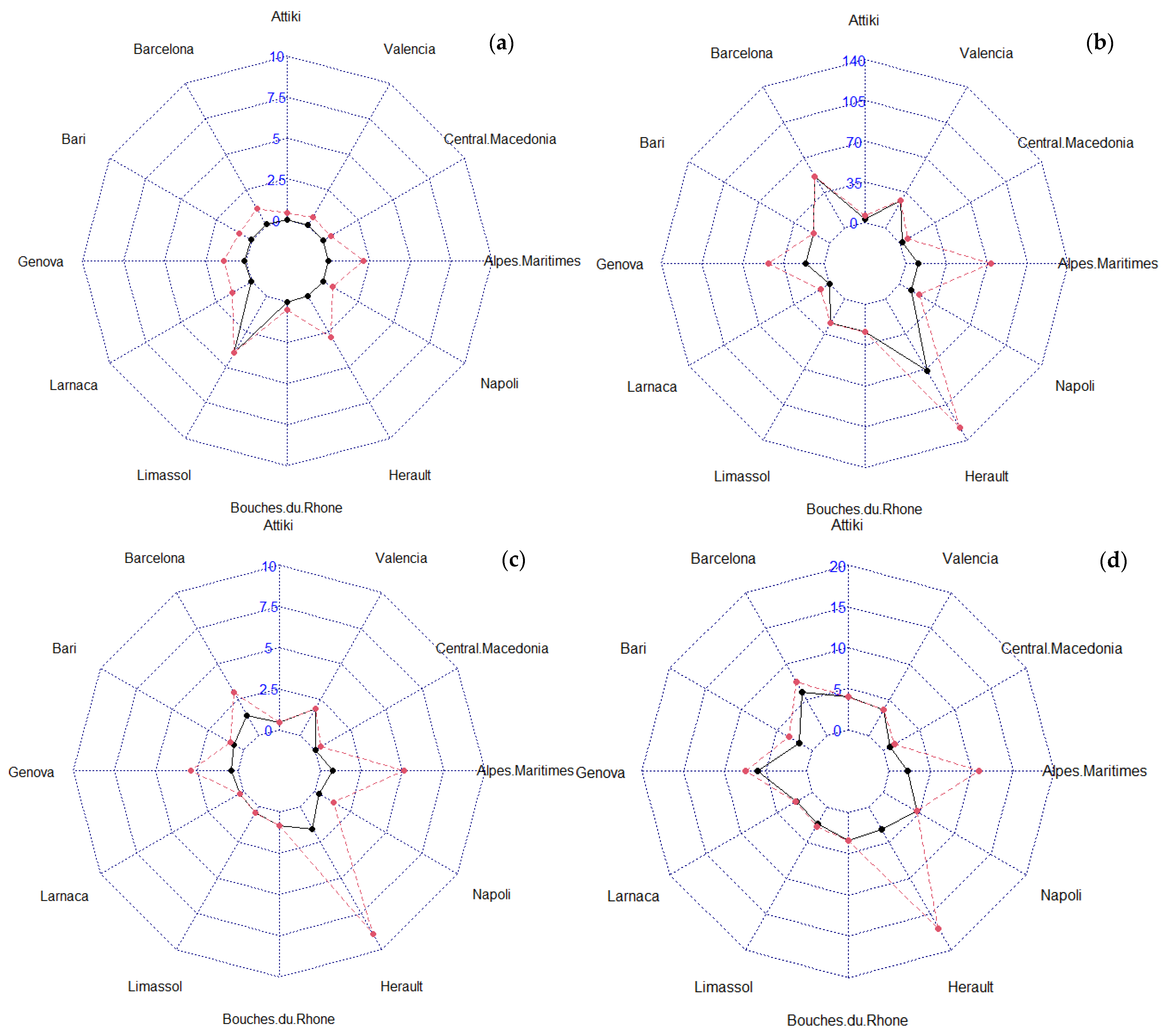
Therefore, Figure 5 presents the targeted values that every under-performing region should reach to achieve its best performance concerning the 4 KPIs. As can be seen from this figure, the regions that have to make the most significant effort to improve their performance in terms of urban growth are Herault, followed by the Alpes-Maritimes. The suggested strategy for improving the current urban growth model that the regions are following is by observing and adapting policies and development strategies that the best-performing regions are already following, especially in cases where the best practitioners exist in the same country.
5. Discussion and Conclusions
Urban growth is a rapidly growing phenomenon that has been investigated countless times in order to understand it and prevent the negative impacts that it has, such as air pollution, poverty, a lack of road safety [40,41] and others. Urban growth rates and spatial patterns of urban development will indeed affect societal, financial and other characteristics of the regions and vice versa. The population growth in urban areas causes an increasing need for housing and urban development and thus a land limitation due to the conversion to housing fact that also affects land pricing (increase in land prices) [42]. Therefore, this forces the residents to move outside the urban cores, thus forming the phenomenon of sprawl cities. However, due to the limitation of space along the coastlines, cities’ expansion does not follow the same trend as inland areas. Additionally, expansion along coastal areas has its consequences in terms of coastal exposure, which should be incorporated into the planning component of city planners [43].
The current paper studies the spatial spillover effect on the urban growth structure of 12 EU coastal regions from five different EU countries and evaluates their current performance in terms of urban growth by implementing different benchmarking techniques. In detail, this study investigates and estimates the performance of the coastal regions in terms of their urban structure in relation to their transport infrastructure, demographic context and landscape (coastline).
The purpose of selecting coastal areas was due to the limitations of expansion that coastal areas have due to their landscape. Based on Figure 1, some of the coastal regions that are following urban development along the coast are Valencia, while other regions are following a mixed development structural model, i.e., along the coastline and inland development (e.g., Bari). Therefore, based on the landscape of the regions (coastline) and their context, it is important to analyze their existing urban growth in order to understand which structure different regions are following. Additionally, the reason for selecting these regions is the coverage of a wide area in Europe and the search for similarities or differences regarding their planning and structural models.
The data collection process focused on collecting information that can adequately capture urban growth, which can be differentiated into different spatial patterns, such as edge compact enlargement of the regions’ boundaries following the main road network and new urbanizations alongside the coast [44]. However, the data collection process of this study faced several limitations due to a lack of information (e.g., financial context of the regions). However, this limitation was overcome because the collected information can provide an adequate “picture” of the region’s urban growth. Additionally, the lack of temporal information made some limitations on dynamically studying the urban growth structure of the regions. However, once again, this analysis provided an overall “picture” of the regions’ existing situation in terms of urban structure.
Therefore, for the evaluation of these nine regions’ KPIs, each one provided a “picture” of the region’s urban structure. However, the combination of some KPIs (e.g., KPIs 2, 3 and 4) showed an indication of denser (e.g., Barcelona) and sprawler areas (e.g., Napoli). Furthermore, the correlation analysis alongside the KPIs 2, 3 and 4 showed that as the coastline of the regions increases, their residential area also increases, which probably will lead to sprawl development. In addition, coastal areas with larger coastlines tend to have larger industrial areas, which might be interpreted as larger industrial ports. The KPIs 7, 8 and 9 are representative of the regions’ transport infrastructure, which appeared to have a relationship to the urban growth of the regions.
In this analysis, more than one region of the same country was investigated in order to see how heterogeneous the regions are in terms of their urban growth performance. Furthermore, each of the regions selected based on the criteria of having at least one port or one airport can be considered as factors that affect urban development [45]. Therefore, the next analysis considered that urban growth is also spatially dependent on not only the regions of the same country but also with distant location, which might be directly or indirectly connected through multimodes (roadway, airway and waterway). The incorporation of this spatial spillover effect of urban growth with the transportation infrastructure, demographic context and landscape (coastline length) of the regions was implemented by the development of a spatially extended DEA model, namely SDEA. Additionally, in similar studies, it appeared that the DEA method used for estimating efficiency scores with spatial data is inappropriate when the regions’ efficiency score is related to the performance of neighboring regions [46]. In this study, the regions are considered connected due to the available multimodes (roadway, airway and waterway).
Different SDEA models were developed, each one analyzing different outputs (KPIs that are identified as spatially dependent based on Moran’s I Test). Based on the results of the SDEA models, Limassol, Bouches-du-Rhône and Valencia appeared to perform best in three out of four models. In detail, Limassol was the only region to perform best- in terms of its urban growth based on KPI 1. Bouches-du-Rhône and Valencia best regarding the KPIs that focused on their transport infrastructure. Therefore, the combination of all SDEA models’ outcomes provides a robust overview “picture” of the regions current urban structure and answers the question of whether the regions have a denser or sprawlier structure and if the regions promote micromobility and public transport, which have a direct impact on the region’s urban growth.
Besides the benchmarking valuation, this study also identifies the targets that every under-performing region should have in terms of the 4 KPIs in order to perform best. Therefore, local authorities in Herault and Alpes-Maritime should revise the existing structural models that they follow for better planning processes in order to prevent sprawl phenomena either along the coastline or inland.
Therefore, this study presented a thorough investigation of the coastal regions’ performance in terms of urban development and appeared to show that coastline is indeed related to urban development and that the combination of KPIs also provides a robust observation of the structural development that the regions are following. The SDEA method is a trustworthy approach for evaluating the regions by incorporating the spatial spillover effects that urban growth has on the regions. Last but not least, the target-setting approach provides guidelines to local authorities and policymakers on the strategies that can be followed towards the regions’ improvements.
Following the above, it is important for local authorities and policymakers to ensure spatial continuity and its integration into the broader urban environment by following different strategies, such as controlling coastal urbanization and planning public spaces through sustainable interventions on a small scale along the coastline [47].
A future study will focus on the incorporation of the demographic and financial contexts of the regions based on the 2021 census. However, data limitations still prevent this implementation. Additionally, in future studies, a larger sample of regions will be incorporated, not only in Europe but as a global sample, for observing homogeneities and heterogeneities between the regions’ urban structures. All the above implementations will incorporate the spatial spillover effects that exist between even distant locations regarding their urban growth.
Author Contributions
Conceptualization, P.N. and S.B.; methodology, P.N. and S.B.; Software, P.N.; Validation, P.N.; Formal Analysis, P.N.; Ιinvestigation, P.N.; Resources, P.N.; Data Curation, P.N.; Writing—original draft preparation, P.N.; Writing—review and editing, P.N. and S.B.; Visualization, P.N.; Supervision, S.B. All authors have read and agreed to the published version of the manuscript.
Funding
This research received no external funding.
Data Availability Statement
Data sharing not applicable.
Conflicts of Interest
The authors declare no conflict of interest.
References
- Population Growth (Annual %)—European Union World Bank Open Data. Available online: https://data.worldbank.org/indicator/SP.POP.GROW?locations=EU (accessed on 27 April 2023).
- Urban Population—European Union|Data. Available online: https://data.worldbank.org/indicator/SP.URB.TOTL?locations=EU (accessed on 27 April 2023).
- The World Bank. Urban Development. 2017. Available online: https://www.worldbank.org/en/topic/urbandevelopment/overview (accessed on 27 April 2023).
- Aljoufie, M.; Brussel, M.; Zuidgeest, M.; van Maarseveen, M. Urban growth and transport infrastructure interaction in Jeddah between 1980 and 2007. Int. J. Appl. Earth Obs. Geoinf. 2013, 21, 493–505. [Google Scholar] [CrossRef]
- Meyer, M.; Miller, E. Urban Transportation Planning; McGraw Hill: New York, NY, USA, 2001. [Google Scholar]
- Hart, T. Transport and the City. In Handbook of Urban Studies; Paddison, R., Ed.; SAGE Publications Ltd.: London, UK; Thousand Oaks, CA, USA; New Delhi, India, 2001. [Google Scholar]
- Cervero, R. Road expansion, urban growth, and induced travel: A Path Analysis. J. Am. Plan. Assoc. 2003, 69, 145–163. [Google Scholar] [CrossRef]
- Cameron, I.; Lyons, T.; Kenworthy, J. Trends in vehicle kilometres of travel in world cities, 1960–1990: Underlying drivers and policy responses. Transp. Policy 2004, 11, 287–298. [Google Scholar] [CrossRef]
- Millot, M. Urban growth, travel practices and evolution of road safety. J. Transp. Geogr. 2004, 12, 207–218. [Google Scholar] [CrossRef]
- Brueckner, J.K. Urban Sprawl: Diagnosis and Remedies. Int. Reg. Sci. Rev. 2000, 23, 160–171. [Google Scholar] [CrossRef]
- Allen, J.; Lu, K. Modeling and Prediction of Future Urban Growth in the Charleston Region of South Carolina: A GIS-based Integrated Approach. Conserv. Ecol. 2003, 8, 2. [Google Scholar] [CrossRef]
- Perveen, S.; Yigitcanlar, T.; Kamruzzaman; Hayes, J. Evaluating transport externalities of urban growth: A critical review of scenario-based planning methods. Int. J. Environ. Sci. Technol. 2016, 14, 663–678. [Google Scholar] [CrossRef]
- Zhang, L.; Zhang, L.; Liu, X. Evaluation of Urban Spatial Growth Performance from the Perspective of a Polycentric City: A Case Study of Hangzhou. Land 2022, 11, 1173. [Google Scholar] [CrossRef]
- Wang, J.; Zhou, J. Spatial evaluation of the accessibility of public service facilities in Shanghai: A community differentiation perspective. PLoS ONE 2022, 17, e0268862. [Google Scholar] [CrossRef]
- Ji, J.; Wang, D. Regional differences, dynamic evolution, and driving factors of tourism development in Chinese coastal cities. Ocean Coast. Manag. 2022, 226, 106262. [Google Scholar] [CrossRef]
- Doerr, L.; Dorn, F.; Gaebler, S.; Potrafke, N. How new airport infrastructure promotes tourism: Evidence from a synthetic control approach in German regions. Reg. Stud. 2020, 54, 1402–1412. [Google Scholar] [CrossRef]
- Boulos, J. Sustainable Development of Coastal Cities-Proposal of a Modelling Framework to Achieve Sustainable City-Port Connectivity. Procedia—Soc. Behav. Sci. 2016, 216, 974–985. [Google Scholar] [CrossRef]
- Kityuttachai, K.; Tripathi, N.K.; Tipdecho, T.; Shrestha, R. CA-Markov Analysis of Constrained Coastal Urban Growth Modeling: Hua Hin Seaside City, Thailand. Sustainability 2013, 5, 1480–1500. [Google Scholar] [CrossRef]
- Nikolaou, P.; Basbas, S.; Politis, I.; Borg, G. Trip and Personal Characteristics towards the Intention to Cycle in Larnaca, Cyprus: An EFA-SEM Approach. Sustainability 2020, 12, 4250. [Google Scholar] [CrossRef]
- Amprasi, V.; Politis, I.; Nikiforiadis, A.; Basbas, S. Comparing the microsimulated pedestrian level of service with the users’ perception: The case of Thessaloniki, Greece, coastal front. Transp. Res. Procedia 2020, 45, 572–579. [Google Scholar] [CrossRef]
- Tzanni, O.; Nikolaou, P.; Giannakopoulou, S.; Arvanitis, A.; Basbas, S. Social Dimensions of Spatial Justice in the Use of the Public Transport System in Thessaloniki, Greece. Land 2022, 11, 2032. [Google Scholar] [CrossRef]
- Vaz, E.d.N.; Nijkamp, P.; Painho, M.; Caetano, M. A multi-scenario forecast of urban change: A study on urban growth in the Algarve. Landsc. Urban Plan. 2012, 104, 201–211. [Google Scholar] [CrossRef]
- Sdoukopoulos, A.; Pitsiava-Latinopoulou, M.; Basbas, S.; Papaioannou, P. Measuring progress towards transport sustainability through indicators: Analysis and metrics of the main indicator initiatives. Transp. Res. Part D Transp. Environ. 2018, 67, 316–333. [Google Scholar] [CrossRef]
- Aljoufie, M.; Zuidgeest, M.; Brussel, M.; van Maarseveen, M. Spatial–temporal analysis of urban growth and transportation in Jeddah City, Saudi Arabia. Cities 2012, 31, 57–68. [Google Scholar] [CrossRef]
- Boeing, G.; Higgs, C.; Liu, S.; Giles-Corti, B.; Sallis, J.F.; Cerin, E.; Lowe, M.; Adlakha, D.; Hinckson, E.; Moudon, A.V.; et al. Using open data and open-source software to develop spatial indicators of urban design and transport features for achieving healthy and sustainable cities. Lancet Glob. Health 2022, 10, e907–e918. [Google Scholar] [CrossRef]
- Dur, F.; Yigitcanlar, T. Assessing land-use and transport integration via a spatial composite indexing model. Int. J. Environ. Sci. Technol. 2014, 12, 803–816. [Google Scholar] [CrossRef]
- Dur, F.; Yigitcanlar, T.; Bunker, J. A Spatial-Indexing Model for Measuring Neighbourhood-Level Land-Use and Transport Integration. Environ. Plan. B Plan. Des. 2014, 41, 792–812. [Google Scholar] [CrossRef]
- Nikolaou, P.; Dimitriou, L. Lessons to be Learned from Top-50 Global Container Port Terminals Efficiencies: A Multi-Period DEA-Tobit Approach. Marit. Transp. Res. 2021, 2, 100032. [Google Scholar] [CrossRef]
- Olejnik, A.; Żółtaszek, A.; Olejnik, J. Spatial Solution to Measure Regional Efficiency—Introducing Spatial Data Envelopment Analysis. Econ. Reg. 2021, 17, 1166–1180. [Google Scholar] [CrossRef]
- Desai, A.; Storbeck, J.E. A data envelopment analysis for spatial efficiency. Comput. Environ. Urban Syst. 1990, 14, 145–156. [Google Scholar] [CrossRef]
- Anselin, A.L.; Rey, S.J. (Eds.) Perspectives on Spatial Data Analysis. In Perspectives on Spatial Data Analysis; Advances in Spatial Science; Springer: Berlin/Heidelberg, Germany, 2010; ISBN 978-3-642-01976-0. [Google Scholar]
- Bogetoft, P.; Otto, L. Benchmarking with DEA, SFA, and R; Springer: New York, NY, USA, 2011. [Google Scholar]
- Charnes, A.; Cooper, W.W.; Rhodes, E. Measuring the efficiency of decision making units. Eur. J. Oper. Res. 1978, 2, 429–444. [Google Scholar] [CrossRef]
- Sherman, H.D.; Zhu, J. Service Productivity Management: Improving Service Performance Using Data Envelopment Analysis (DEA); Springer Science+Business Media, LLC.: New York, NY, USA, 2006. [Google Scholar]
- Cooper, W.W.; Seiford, L.M.; Tone, K. Data Envelopment Analysis: A Comprehensive Text with Models, Applications, References and DEA-Solver Software, 2nd ed.; Springer Science+Business Media, LLC.: New York, NY, USA, 2007. [Google Scholar]
- GHSL—Global Human Settlement Layer. Global Human Settlement—Download—European Commission. 2016. Available online: https://ghsl.jrc.ec.europa.eu/download.php?ds=pop (accessed on 5 May 2023).
- OpenStreetMap. 2022. Available online: https://www.openstreetmap.org/copyright (accessed on 1 May 2023).
- Navigation (No Date) Transport Networks—GISCO—Eurostat. Available online: https://ec.europa.eu/eurostat/web/gisco/geodata/reference-data/transport-networks (accessed on 5 May 2023).
- Natural Earth—Free Vector and Raster Map Data at 1:10m, 1:50m, and 1:110m Scales. Available online: https://www.naturalearthdata.com (accessed on 5 May 2023).
- Urbanization Effects. Environment. 2021. Available online: https://www.nationalgeographic.com/environment/article/urban-threats (accessed on 1 August 2023).
- Henning-Hager, U. Urban development and road safety. Accid. Anal. Prev. 1986, 18, 135–145. [Google Scholar] [CrossRef]
- Suwarlan, S.A.; Lee, Y.L.; Said, I. A review of agricultural and coastal cities in indonesia in finding urban sprawl priority parameters. Modul 2022, 22, 91–99. [Google Scholar] [CrossRef]
- Wolff, C.; Nikoletopoulos, T.; Hinkel, J.; Vafeidis, A.T. Future urban development exacerbates coastal exposure in the Mediterranean. Sci. Rep. 2020, 10, 14420. [Google Scholar] [CrossRef]
- Aguilar, J.A.P.; Añó, V.A.C.; Sánchez, J. Urban growth dynamics (1956–1998) in mediterranean coastal regions: The case of alicante, spain. In Desertification in the Mediterranean Region. A Security Issue; Springer: Dordrecht, The Netherlands, 2006; pp. 325–340. [Google Scholar]
- Inouye, C.E.N.; de Sousa, W.C.; de Freitas, D.M.; Simões, E. Modelling the spatial dynamics of urban growth and land use changes in the north coast of São Paulo, Brazil. Ocean Coast. Manag. 2015, 108, 147–157. [Google Scholar] [CrossRef]
- Ramajo, J.; Marquez, M.; Hewings, G. Addressing spatial heterogeneity in Regional Technical Efficiency. SSRN Electron. J. 2020. [Google Scholar] [CrossRef]
- Theodora, Y.; Spanogianni, E. Assessing coastal urban sprawl in the Athens’ southern waterfront for reaching sustainability and resilience objectives. Ocean Coast. Manag. 2022, 222, 106090. [Google Scholar] [CrossRef]
Figure 1.
Flowchart of methodological framework.
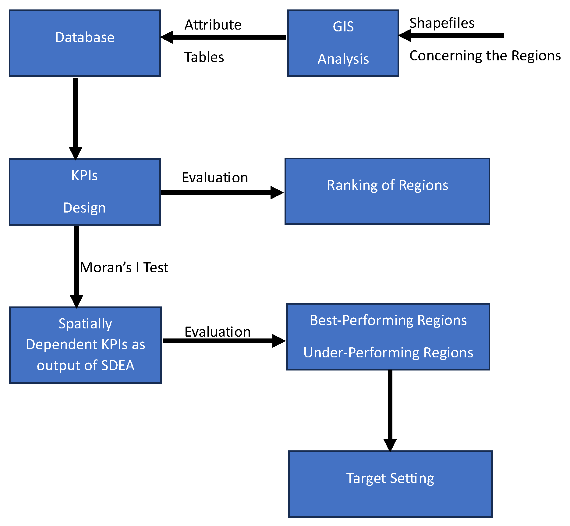
Figure 2.
Study area: 12 EU regions of 5 European Union countries [36] that where considered to have a spatial connection.
Figure 2.
Study area: 12 EU regions of 5 European Union countries [36] that where considered to have a spatial connection.
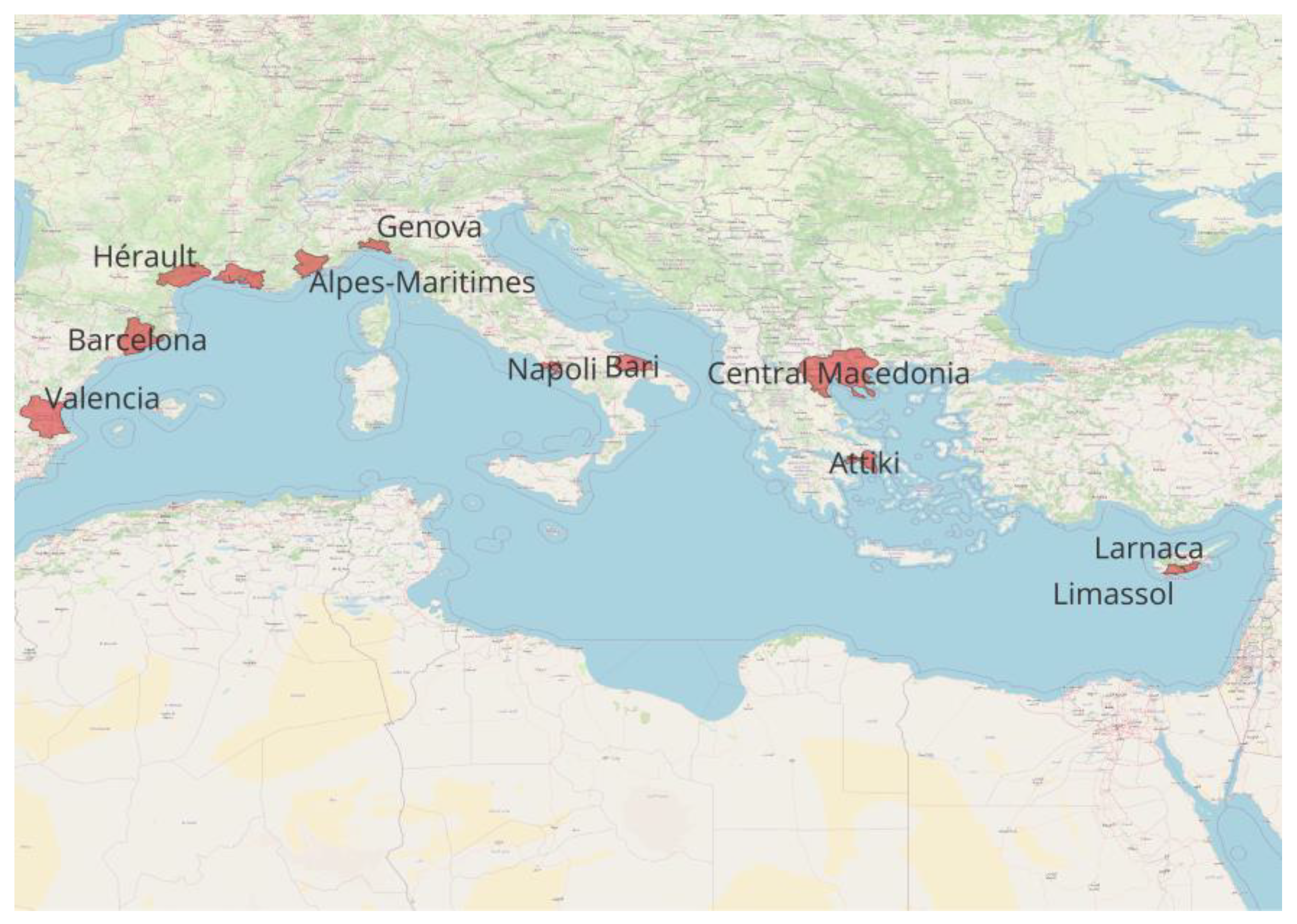
Figure 3.
Correlation analysis of concluded database.

Figure 4.
Population distribution of the 12 EU regions (scale for sparse areas: white to dense areas: black).
Figure 4.
Population distribution of the 12 EU regions (scale for sparse areas: white to dense areas: black).
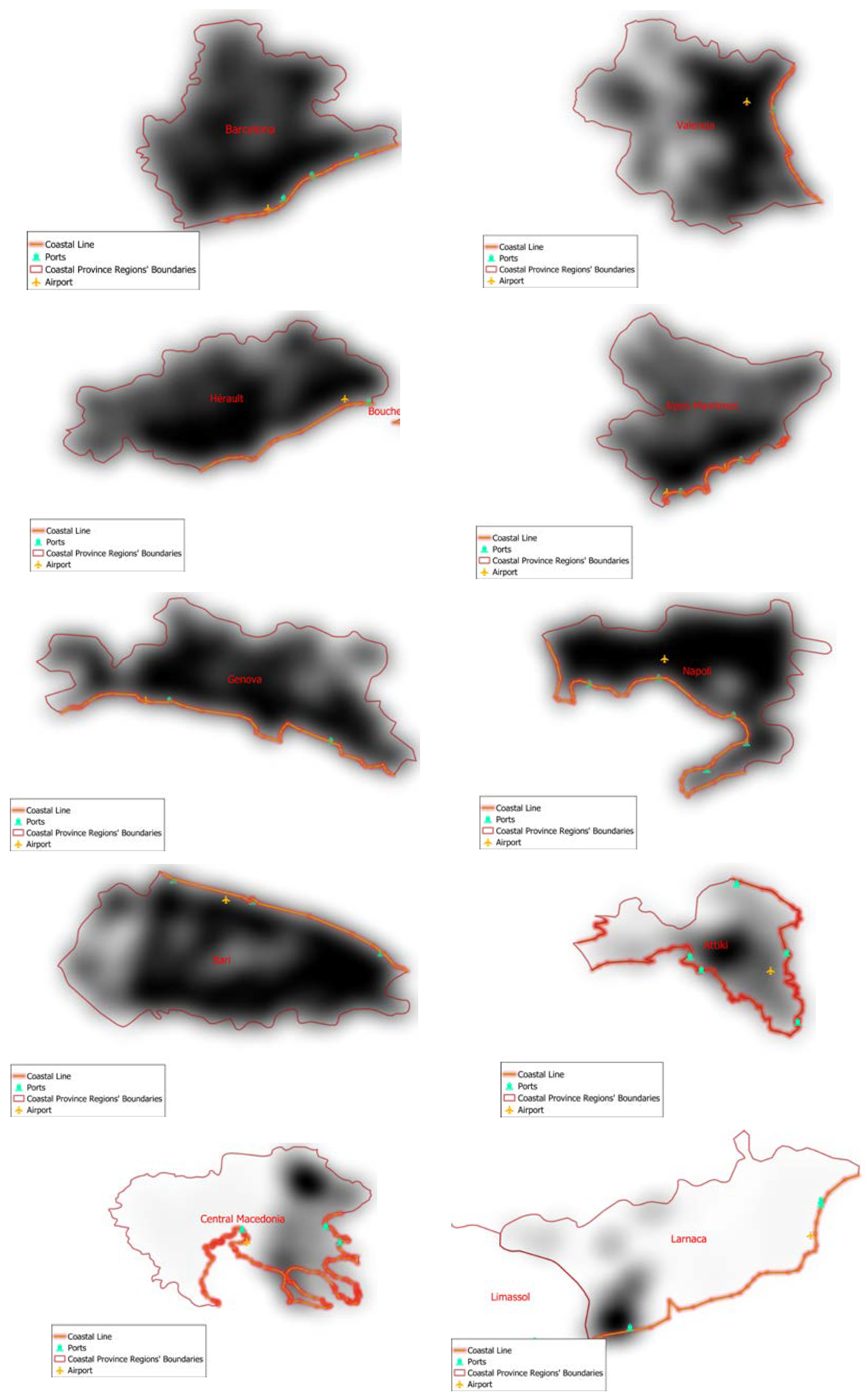
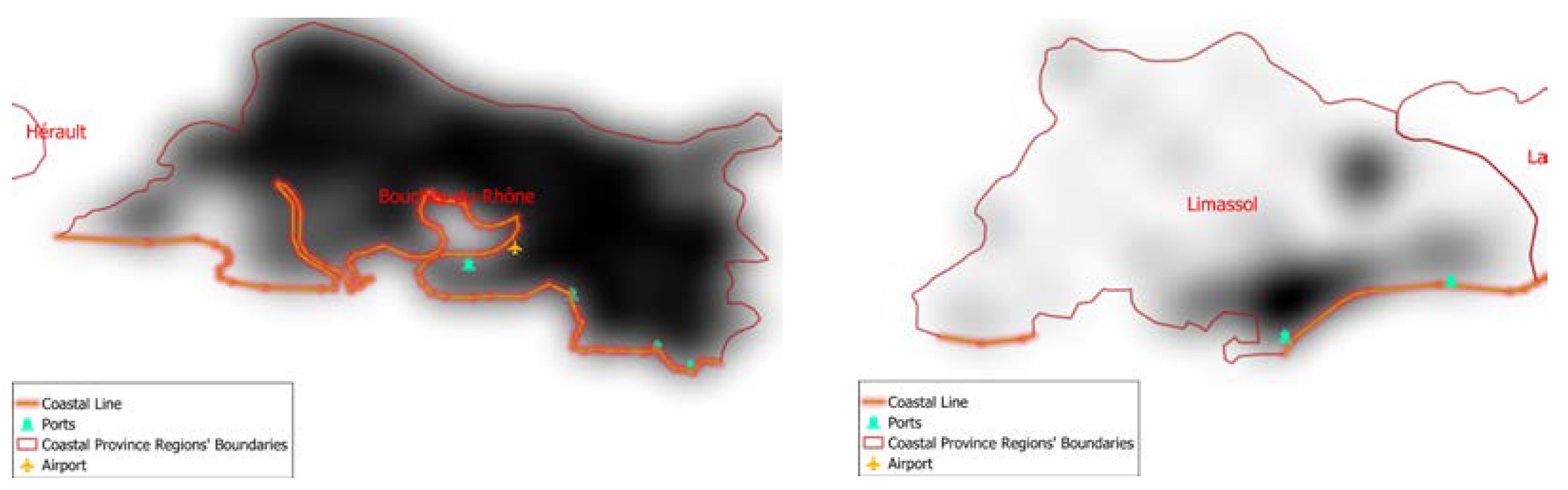
Figure 5.
Targets setting approach for improving under-performing coastal regions based on: (a) KPI 1; (b) KPI 2; (c) KPI 3; and (d) KPI 4 (targeted values: red dashed line; existing values: black line).
Figure 5.
Targets setting approach for improving under-performing coastal regions based on: (a) KPI 1; (b) KPI 2; (c) KPI 3; and (d) KPI 4 (targeted values: red dashed line; existing values: black line).

Table 1.
Geoinformation Collected Concerning the 12 EU Regions in 5 European Union Countries.
| Variable | Description | Measure Unit | Source |
|---|---|---|---|
| Tot_Pop | Total residential population | Total number of people | European Commision [36] |
| Road_length | Length of road infrastructure | Kilometers | OpenStreetMaps [37] |
| Cycleway_length | Length of cycleway | Kilometers | OpenStreetMaps [37] |
| Ped_length | Length pedestrian infrastructure | Kilometers | OpenStreetMaps [37] |
| PT_length | Length of public transportation network | Kilometers | OpenStreetMaps [37] |
| Num_POIs | Points of interest | Number of points (e.g., tourist attractions shopping areas, religious sites) | OpenStreetMaps [37] |
| Num_Build | Buildings | Number of buildings (e.g., hotels, residential, offices) | OpenStreetMaps [37] |
| Build_area | Building area | Square kilometers | OpenStreetMaps [37] |
| Res_build_area | Area of buildings inside residential land | Square kilometers | OpenStreetMaps [37] |
| Park_loc | Locations with parking | Number of parking locations | OpenStreetMaps [37] |
| Airports | Location of airports | Number of airports | Euostat [38] |
| Ports | Location of ports | Number of ports | Euostat [38] |
| Res_area | Residential area | Square kilometers | OpenStreetMaps [37] |
| Com_area | Commercial area | Square kilometers | OpenStreetMaps [38] |
| Ind_area | Industrial area | Square kilometers | OpenStreetMaps [38] |
| PT_infra | Public transport infrastructure | Number of bus stops, railway stations, platforms, tram stops | OpenStreetMaps [38] |
| Region_area | Total area of the region | Square kilometers | Natural Earth [39] |
| Coast_length | Coastal line length | Kilometers | Natural Earth [39] |
Table 2.
Key performance indicators.
| KPI | Value | Measure Unit |
|---|---|---|
| KPI 1: Buildings’ capacity | Tot_Pop/Res_build_area | People per sqr. meters of residential buildings’ area |
| KPI 2: Population density | Tot_Pop/Res_area | People per sqr. meters of residential area |
| KPI 3: Building’ coverage | Res_build_area/Res_area | % of covered residential area from the buidings’ area |
| KPI 4: Residential area coverage | Res_area/Region_area | % of residential area to the total area of the region |
| KPI 5: Commercial area coverage | Com_area/Region_area | % of commercial area to the total area of the region |
| KPI 6: Industrial area coverage | Ind_area/Region_area | % of industrial area to the total area of the region |
| KPI 7: Public transport infrastructure | PT_length/ Road_length | % of public transportation length compared to total road length |
| KPI 8: Cycling infrastructure | Cycleway_length/ Road_length | % of cycleway length compared to total road length |
| KPI 9: Walking infrastructure | Ped_length/ Road_length | % of pedestrian pathway length compared to total road length |
Table 3.
Results of the KPIs.
| Region | Country | KPI1 | KPI2 | KPI3 | KPI4 | KPI5 | KPI6 | KPI7 | KPI8 | KPI9 |
|---|---|---|---|---|---|---|---|---|---|---|
| Hérault | France | 0.018 (12) | 0.003 (12) | 16.35 (5) | 6.39 (8) | 0.08 (7) | 0.55 (5) | 71.48 (1) | 1.55 (2) | 3.92 (7) |
| Bouches-du-Rhône | France | 0.029 (11) | 0.004 (9) | 14.32 (6) | 9.09 (9) | 0.16 (10) | 2.41 (11) | 24.01 (6) | 0.84 (4) | 4.29 (6) |
| Alpes-Maritimes | France | 0.032 (10) | 0.003 (11) | 8.16 (9) | 9.41 (10) | 0.69 (12) | 0.49 (4) | 10.85 (8) | 0.78 (5) | 2.83 (9) |
| Larnaca | Cyprus | 0.051 (9) | 0.003 (10) | 5.37 (11) | 5.48 (6) | 0.05 (5) | 0.59 (6) | 0.00 (12) | 0.24 (11) | 2.79 (10) |
| Central Macedonia | Greece | 0.059 (8) | 0.004 (8) | 6.49 (10) | 2.37 (3) | 0.02 (3) | 0.25 (2) | 1.78 (10) | 0.06 (12) | 1.15 (12) |
| Attiki | Greece | 0.061 (7) | 0.010 (6) | 16.77 (4) | 11.82 (12) | 0.10 (8) | 1.54 (9) | 3.30 (9) | 0.43 (7) | 4.99 (4) |
| Valencia | Spain | 0.063 (6) | 0.008 (7) | 12.47 (7) | 2.91 (4) | 0.04 (4) | 0.95 (8) | 27.15 (5) | 1.90 (1) | 4.50 (5) |
| Napoli | Italy | 0.087 (5) | 0.026 (4) | 29.41 (1) | 10.21 (11) | 0.27 (11) | 2.51 (12) | 70.65 (2) | 0.26 (10) | 5.76 (3) |
| Bari | Italy | 0.139 (4) | 0.033 (3) | 23.97 (3) | 0.96 (2) | 0.06 (6) | 0.74 (7) | 38.21 (4) | 0.67 (6) | 2.27 (11) |
| Barcelona | Spain | 0.157 (3) | 0.014 (5) | 8.86 (8) | 5.64 (7) | 0.12 (9) | 2.04 (10) | 51.17 (3) | 1.39 (3) | 7.67 (1) |
| Genova | Italy | 0.287 (2) | 0.072 (2) | 25.12 (2) | 0.56 (1) | 0.01 (1) | 0.21 (1) | 16.03 (7) | 0.40 (9) | 7.49 (2) |
| Limassol | Cyprus | 7.938 (1) | 0.405 (1) | 5.10 (12) | 4.52 (5) | 0.01 (2) | 0.37 (3) | 0.00 (11) | 0.41 (8) | 2.92 (8) |
Note: Parenthesis denotes the ranking position of the regions based on each different KPI.
Table 4.
Significance of Moran’s I Test.
| KPIs | Moran’s I Test Significance (p-Value) | Z-Score | Interpretation |
|---|---|---|---|
| KPI 1 | 0.05 | 1.63 | Spatial Dependence |
| KPI 2 | 0.08 | 1.42 | Spatial Independence |
| KPI 3 | 0.41 | 0.22 | Spatial Independence |
| KPI 4 | 0.75 | −0.69 | Spatial Independence |
| KPI 5 | 0.61 | −0.28 | Spatial Independence |
| KPI 6 | 0.25 | 0.68 | Spatial Independence |
| KPI 7 | 0.05 | 1.62 | Spatial Dependence |
| KPI 8 | 0.00 | 3.65 | Spatial Dependence |
| KPI 9 | 0.03 | 1.91 | Spatial Dependence |
Table 5.
Results of the SDEA models.
| Region (Country) | Output: KPI1 Efficiency | Output: KPI7 Efficiency | Output: KPI8 Efficiency | Output: KPI9 Efficiency |
|---|---|---|---|---|
| Attiki (Greece) | 13.97 | 2.31 | 1.00 | 1.00 |
| Barcelona (Spain) | 14.68 | 1.00 | 2.18 | 1.23 |
| Bari (Italy) | 12.54 | 1.19 | 1.42 | 1.82 |
| Genova (Italy) | 9.53 | 1.00 | 7.05 | 1.25 |
| Larnaca (Cyprus) | 54.24 | 12142.76 | 1.09 | 1.03 |
| Limassol (Cyprus) | 1.00 | 1.00 | 1.00 | 1.15 |
| Bouches-du-Rhône (France) | 33.84 | 1.00 | 1.00 | 1.00 |
| Hérault (France) | 319.55 | 2.33 | 5.76 | 5.42 |
| Napoli (Italy) | 15.73 | 1.85 | 4.97 | 1.00 |
| Alpes-Maritimes (France) | 136.32 | 1.00 | 6.56 | 4.83 |
| Central Macedonia (Greece) | 18.64 | 5.06 | 7.51 | 1.66 |
| Valencia (Spain) | 18.90 | 1.00 | 1.00 | 1.00 |
Disclaimer/Publisher’s Note: The statements, opinions and data contained in all publications are solely those of the individual author(s) and contributor(s) and not of MDPI and/or the editor(s). MDPI and/or the editor(s) disclaim responsibility for any injury to people or property resulting from any ideas, methods, instructions or products referred to in the content. |
© 2023 by the authors. Licensee MDPI, Basel, Switzerland. This article is an open access article distributed under the terms and conditions of the Creative Commons Attribution (CC BY) license (https://creativecommons.org/licenses/by/4.0/).
Share and Cite
MDPI and ACS Style
Nikolaou, P.; Basbas, S. Urban Development and Transportation: Investigating Spatial Performance Indicators of 12 European Union Coastal Regions. Land 2023, 12, 1757. https://doi.org/10.3390/land12091757
AMA Style
Nikolaou P, Basbas S. Urban Development and Transportation: Investigating Spatial Performance Indicators of 12 European Union Coastal Regions. Land. 2023; 12(9):1757. https://doi.org/10.3390/land12091757
Chicago/Turabian StyleNikolaou, Paraskevas, and Socrates Basbas. 2023. "Urban Development and Transportation: Investigating Spatial Performance Indicators of 12 European Union Coastal Regions" Land 12, no. 9: 1757. https://doi.org/10.3390/land12091757
Note that from the first issue of 2016, this journal uses article numbers instead of page numbers. See further details here.