Article

Assessing the Impacts of Climate and Land Use Change on Water Conservation in the Three-River Headstreams Region of China Based on the Integration of the InVEST Model and Machine Learning

1
State Key Laboratory of Hydraulics and Mountain River Engineering, Sichuan University, Chengdu 610065, China
2
Gansu Province Water Resources and Hydropower Survey Design Institute Co., Ltd., Lanzhou 730000, China
*
Author to whom correspondence should be addressed.
Land 2024, 13(3), 352; https://doi.org/10.3390/land13030352
Submission received: 25 January 2024 / Revised: 1 March 2024 / Accepted: 2 March 2024 / Published: 8 March 2024
(This article belongs to the Special Issue Feature Papers for Land–Climate Interactions Section II)

Abstract

:
The Three-River Headstreams Region (TRHR) serves as the cradle of China’s three major rivers—the Yangtze, Yellow, and Lancang—rendering its water conservation (WC) capacity quintessentially significant for Asian water resource security. This study integrated the InVEST model and random forest model to holistically elucidate the spatiotemporal characteristics and factors influencing WC in the TRHR from 1980 to 2018. The results revealed that the WC growth rate was 5.65 mm/10a in the TRHR during the study period, yet pronounced regional disparities were observed among different basins, especially with the Lancang River Basin (LRB), which exhibited a decrease at a rate of 5.08 mm per decade despite having the highest WC. Through Theil–Sen trend analysis, the Mann–Kendall abrupt change test, and the cumulative deviation method, meteorological, vegetative, and land use abrupt changes in approximately 2000 were identified as the primary drivers for the abrupt surge in WC within the TRHR. Furthermore, precipitation and the aridity index were the core feature variables affecting WC. However, a positive transition in land use patterns post-2000 was also revealed, and its favorable effect on WC was not as significant as the abrupt climatic changes. This study offers new perspectives on managing multidimensional spatiotemporal data and contributes to laying the groundwork for machine learning applications in water conservation. Additionally, it potentially provides useful references for decision-making processes related to ecosystem security.

1. Introduction

Water conservation (WC), a vital component of ecosystem services, is crucial for maintaining ecological equilibrium and ensuring water supply [1,2,3]. There are numerous methods to quantify WC, including the water balance method, water storage capacity method, and rainfall storage method, along with various estimation models, such as the InVEST model, the SWAT model, and the cellular automata model. Currently, the InVEST model is a comprehensive tool for evaluating multiple ecosystem services and has been extensively utilized in assessing WC [4,5]. Its widespread application is attributed to the ease of data acquisition, flexible parameter adjustment, and spatial expressiveness of evaluation results [6,7,8]. The InVEST model has been extensively utilized across various regions. J.W. Redhead simulated the water yield in 22 river basins in the United Kingdom using the InVEST model and compared the results with data from the UK National River Flow Archive, demonstrating the model’s ability to accurately evaluate WC [9]. Pessacg Natalia applied the InVEST model to simulate the water yield in the Chubut River Basin in Argentina and found that the spatial distribution of precipitation had a significant impact on WC [10]. In addition, the InVEST model has yielded numerous achievements in the areas of WC and water yield in various regions of China, such as the Yellow River Basin (YRB) [11,12,13], Loess Plateau [14], Qinghai–Tibet Plateau [15,16], Yangtze River Basin (YZRB) [17], Danjiang basin [18], Poyang Lake [19], and Dongting Lake [20].
Previous studies predominantly employed conventional methodologies, such as correlation analysis, principal components analysis, or cluster analysis, to explore the drivers behind WC changes [18,20] or utilized scenario-based simulations to gauge the responses of WC to climate and land use alterations [21,22]. However, these methods may have difficulty in dealing with the complexity and multidimensionality of the data, especially when confronted with large-scale spatial data. By harnessing tools such as ArcGIS and Python, we now navigate spatial data more adeptly, streamlining data acquisition, extraction, and analysis. For instance, machine learning (ML) models, with their innate ability to adapt to data intricacies and model nonlinear interactions, have uncovered new avenues for in-depth analyses of complex ecosystems [23]. While machine learning has made significant advances in other areas [24,25,26], its application in WC assessment and ecosystem services remains comparatively unknown [25]. There have been exploratory studies using machine learning models to evaluate the impact of ecological fallow projects on the water conservation capacity of the YRB, but these studies have limited data and insufficient model accuracy [11]. Utilizing ArcGIS, we generated a large amount of spatial sample data, meeting the input data requisites for any ML model, offering a fresh perspective for original data generation, and propelling the use of ML in spatial analyses within the ecosystem services domain.
The TRHR, a global ecological hotspot and a pivotal ecological service hub in the world, offers invaluable insights into WC studies [26,27,28,29]. Diverse methodologies have yielded inconsistent findings on WC trends, influenced by differing study durations and regions. Naveed Ahmed, for example, reported a 22.7% and 12.5% decline in WC capacities in the Yellow and Yangtze River source regions, respectively, between 1961 and 2000, linked to alpine ecosystem degradation [30]. In contrast, Yao Pan’s research observed a southeast TRHR decline but an uptick elsewhere over the past 30 years [31]. While some analyses exist on the spatial–temporal dynamics of WC, the role of vegetation shifts is underexplored [32]. Comprehensive discussions of the various factors influencing WC are scant. Furthermore, a focus on long-term changes is often missing, with fragmented and early time-series studies [33]. Given the expansive and intricate landscape of the TRHR and the interplay between natural and anthropogenic factors leading to pronounced WC disparities, delving into these spatial–temporal dynamics is crucial.
In this context, our study endeavors to harness time trend analysis and ML, particularly the random forest model, to evaluate the WC in the TRHR and delve into its association with meteorological factors, vegetation, and land use, among others. By analyzing a large amount of spatiotemporal sample data, we aim to propose a novel, more accurate, and comprehensive method for assessing the factors influencing the WC dynamics, with the aspiration of furnishing strong support for the assessment and management of WC.

2. Materials and Methods
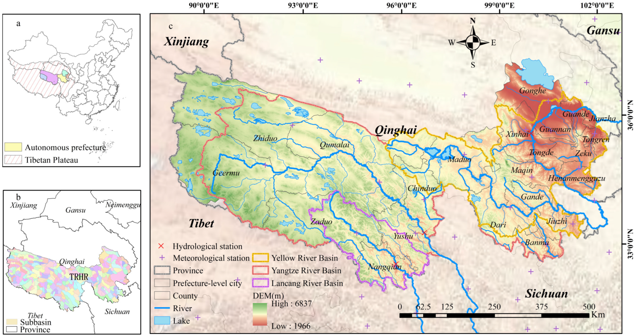
2.1. Study Area

The TRHR, located in southern Qinghai Province, China, encompasses the headwaters of the Yangtze, Yellow, and Lancang Rivers, extending across an area of 375.8 thousand square kilometers (Figure 1). Dominated by a complex terrain, the region descends from northwest to southeast, with elevations ranging between 1966 and 6837 m and an average altitude exceeding 4000 m. It is characterized by a plateau continental climate, manifesting distinct wet and dry seasons, concurrent water and heat periods, prolonged sunlight, and high annual solar radiation. Yearly average temperatures oscillate between −7.75 °C and 9.06 °C, with an annual precipitation span of 161.14 to 723.43 mm [27]. As the cradle of the YZRB, YRB, and LRB, the region hosts a dense river network with over 180 rivers, constituting 4.40% of the total area, and an annual runoff volume of 324.17 × 10³ m3, alongside a multiyear average flow rate of 1022.3 m3/s [34,35]. The diverse topography engenders widespread lakes and marshes, abundant snow mountains and glaciers, with wetlands spanning approximately 73.3 thousand km² and over 1800 lakes. Soil exhibits a vertical zonal distribution, including nine soil orders, such as semileached, calcic, initial, and alpine soils, with alpine meadow soil being predominant. Vegetation primarily consists of cold-resistant grasslands and meadows, covering 47.06% and 16.55% of the area, respectively. The region encompasses 22 counties across five autonomous prefectures (Figure 1) [36].

2.2. Data Sources and Processing Methods

Figure 2 and Table 1 delineate the data sources utilized for WC computation, validation, and contribution. A selection of observational data from 86 meteorological stations, encompassing the study area and its vicinity, was employed (Figure 1). Spatial interpolation via the splina and lapgrd modules in ANUSPLIN version 4.3 yielded annual average temperatures, ensuring that the degrees of freedom postinterpolation remained below half of the interpolating stations, corroborating the validity and scientific rigor of the spatially interpolated data [37]. Annual precipitation spatial data were generated using kriging interpolation. Specialized meteorological interpolation software ANUSPLIN version 4.3 employed a DEM-corrected spatial interpolation method reflecting the vertical variation in temperature and reference crop evapotranspiration.
The manual interpretation of eight epochs of land cover maps was derived from Landsat-MSS/TM/ETM satellite imagery. Based on the TRHR’s natural geographic and cover characteristics, a reclassification of land use types was conducted after operations such as clipping, projecting, and reclassification, culminating in nine land use types (Table A1). A polygon-linking approach on the 1:100,000 scale Second National Soil Survey maps and 8595 soil profile diagrams, coupled with NC format conversion, was utilized to craft 30 m precision soil data incorporating soil depth, soil clay, silt, gravel, and organic matter content information [38].
Based on the GLOBMAP Leaf Area Index (LAI) Version 3 Description, the LAI was obtained with a spatial resolution of 8 km from 1981 to 2018 [39,40]. The National Tibetan Plateau Scientific Data Center supplied the normalized difference vegetation index (NDVI) data spanning the years 1982 to 2015 (Dataset 1) [41], while the Chinese Academy of Sciences Resource and Environment Science and Data Center provided the NDVI data for the interval 1998 to 2018 (Dataset 2). Due to the distinct sensors of the two datasets, a consistency check was imperative, revealing a significant correlation coefficient of 0.851 (p < 0.05). Dataset 2 (1998–2018), with a higher spatial resolution, was selected as the reference, and Dataset 1 (1982–2015) was used to extend the NDVI data sequence for the TRHR from 1982 to 2018. The terrain index was obtained through ArcGIS spatial analysis [42]. The runoff velocity coefficients, which vary with land use change over periods, were adopted from recent studies [18]. The soil saturated hydraulic conductivity in the study area was computed using NeuroTheta software version 1.0.

2.3. Dataset Generation via ArcGIS

ArcGIS software version 10.8 was utilized to construct a 10 km sampling grid within the study area, yielding 11,650 sample points. Subsequently, yearly WC and natural factor values were extracted to these points and exported to an Excel spreadsheet, generating an initial natural factor database. Different land class grid data were converted into polygon files and buffers for sample points were created, and then the area of different land classes for each sample point was computed through intersection tabulation. During the dataset preprocessing phase, null and anomalous values within the area data of different land use types were averaged, culminating in a ML analysis dataset encompassing 9356 spatial points. The final dataset included 16 feature factors, such as annual precipitation (P), average annual temperature (TEM), reference crop evapotranspiration (ET0), actual evapotranspiration (AET), Leaf Area Index (LAI), normalized difference vegetation index (NDVI), and land use and cover change (LUCC), aiming to quantify their impacts on WC (Table 2). Among them, A E T = K c × E T 0 , where Kc is the actual crop coefficient (dimensionless) [43].

2.4. Methods

2.4.1. The InVEST Water Yield Model and Water Conservation Computation

The water yield module accounts for many factors, including precipitation, evapotranspiration, land use type, and plant biophysical characteristics, to obtain the water yield for each grid within the study region and aggregates them to ascertain the water yield for each subbasin within the area [44]. The principles and formulas for the water yield model are in Appendix A.1.
The WC of the TRHR was obtained by considering the topographic index, flow rate coefficient, and soil saturation hydraulic conductivity. The WC was calculated as follows:
W C = min 1 , 249 V e l o c i t y × min 1 , 0.9 × T I 3 × min 1 , K s 300 × Y i e l d ( x )
where WC indicates water conservation, Velocity indicates the flow rate coefficient, TI represents the dimensionless topographic index, Ks is saturated hydraulic conductivity, calculated using Australian NeuroTheta software version 1.0, and Y i e l d ( x ) is the water yield.
T I = ln α tan β
where α indicates the catchment area per unit contour length at any point of the flow through the slope, and tan β is the slope at that point.

2.4.2. Trend Analysis

Initially, this paper employs the Mann–Kendall (M-K) abrupt change analysis method to scrutinize the abrupt features of WC within the TRHR. Following this process, the results computed from the Mann–Kendall abrupt analysis method are validated and supplemented using the cumulative deviation method. The M-K abrupt detection does not necessitate that the sample adhere to a particular distribution pattern and is unaffected by a few outlier values. Through Python programming, the M-K abrupt detection curve was obtained, with the specific curve principle elaborated in Appendix A.2.
The cumulative distance adjustment (CDA) method is another approach for identifying sudden breakpoints between a value and the multiyear average based on the trend of a curve over time. The moment of abrupt change in cumulative distance levels, signifying a different trend from prior observations, marks the time of abrupt changes in time-series data.
L i = i = 1 n ( R i R ¯ )
In this equation, L i stands for cumulative distance from mean value, R i denotes the element value of the ith year, and R ¯ signifies the multiyear average of the element.
The Theil–Sen Trend Analysis is a nonparametric test method utilized in this study for examining the trend variations in WC in TRHR before and after abrupt changes, without necessitating normal distribution and linear trend assumptions, effectively mitigating outliers and missing data noise interference.
β = m e d i a n ( x j x i j i ) , 1 < i < j < n
In the formula, β represents the median slope of all data pairs, where the sign indicates the direction of the trend. A positive β signifies an ascending trend in the series, while a negative value denotes a descending trend. The symbols x j and x i specifically represent the magnitudes of the data at the jth and ith positions in the time series, respectively.

2.4.3. Correlation and Cluster Analysis

The Pearson correlation coefficient r (−1 ≤ r ≤ 1) is obtained by dividing the covariance of two sample data by their standard deviations. It is used to evaluate the degree of linearity between variables and is considered significant at p < 0.05 [45,46]. The Pearson correlation coefficient was used to scrutinize the correlation between the nonnull raster data values of each driver under temporal variation and WC across various regions to assess their response to WC.
Systematic cluster analysis was used to discover the dependencies between the factors. Initially, the driving factors were standardized. To quantify the similarity between factors, a distance metric was needed. The widely used Euclidean distance was applied while employing the efficient Ward’s linkage method for clustering the samples based on the minimal increase in the sum of squares of the dissimilarities among them [47]. This approach enabled the determination of the drivers’ similarity to the water content and the categorization of each driver [48].

2.4.4. Machine Learning Model

The random forest (RF) embodies a sophisticated ensemble learning technique, enhancing the model’s generalization capacity and accuracy through the amalgamation of predictions from multiple decision trees [49]. Within this ensemble structure, each tree is trained on a unique dataset acquired via bootstrap sampling, ensuring diversity throughout the training process [23]. Moreover, the model escalates its resilience against overfitting by selecting the optimum feature from a random subset of features during each node split. In this study, the scikit-learn library’s random forest model was employed, delineating the data into training and testing sets. The model was trained with predefined parameters (e.g., n estimators = 100, denoting 100 trees), and the inherent feature importance attribute was utilized to evaluate the significance of each feature.
In this endeavor, an incremental mean squared error (IncMSE)-based approach was adopted to assess the contribution of each feature to model prediction [50]. Furthermore, the annual indicators’ significance was ranked and iteratively appended to the model input in a sequential manner. During this phase, a fivefold cross-validation was executed to appraise the impact of different feature combinations on model predictive performance [51]. Cross-validation curves unveiled how the model’s accuracy oscillates with the variation in input indicator quantity, aiding in identifying the optimum regression point.

3. Results

3.1. Water Conservation Simulation Results

3.1.1. The Validation Process for the InVEST Model

The water yield module in the InVEST model necessitates the vector boundaries of the area and its subwatersheds; there were 389 subwatersheds in this study. The biophysical coefficient table indicates the main parameters needed for the model, including land attribute parameters, such as LULC, vegetation cover, root depth, and Kc, as shown in Table 3. In this study, we validated the water yield model with the annual runoff modulus of the hydrological station. Validation points were selected at the ZhiMenDa, XiangDa, and TangNaiHai hydrological stations located on the main streams of the Yangtze, Yellow, and Lancang rivers, respectively. The Zhang coefficient was calibrated using the actual annual runoff modulus from 1980 to 2010 compared with the simulated annual water yield by the InVEST model, with the specific simulation results shown in Figure 3a. The results indicated that the model’s water yield simulation was optimal when the Zhang coefficient was 13.2, with a relative error in the model validation results of less than 5% (Figure 3b).

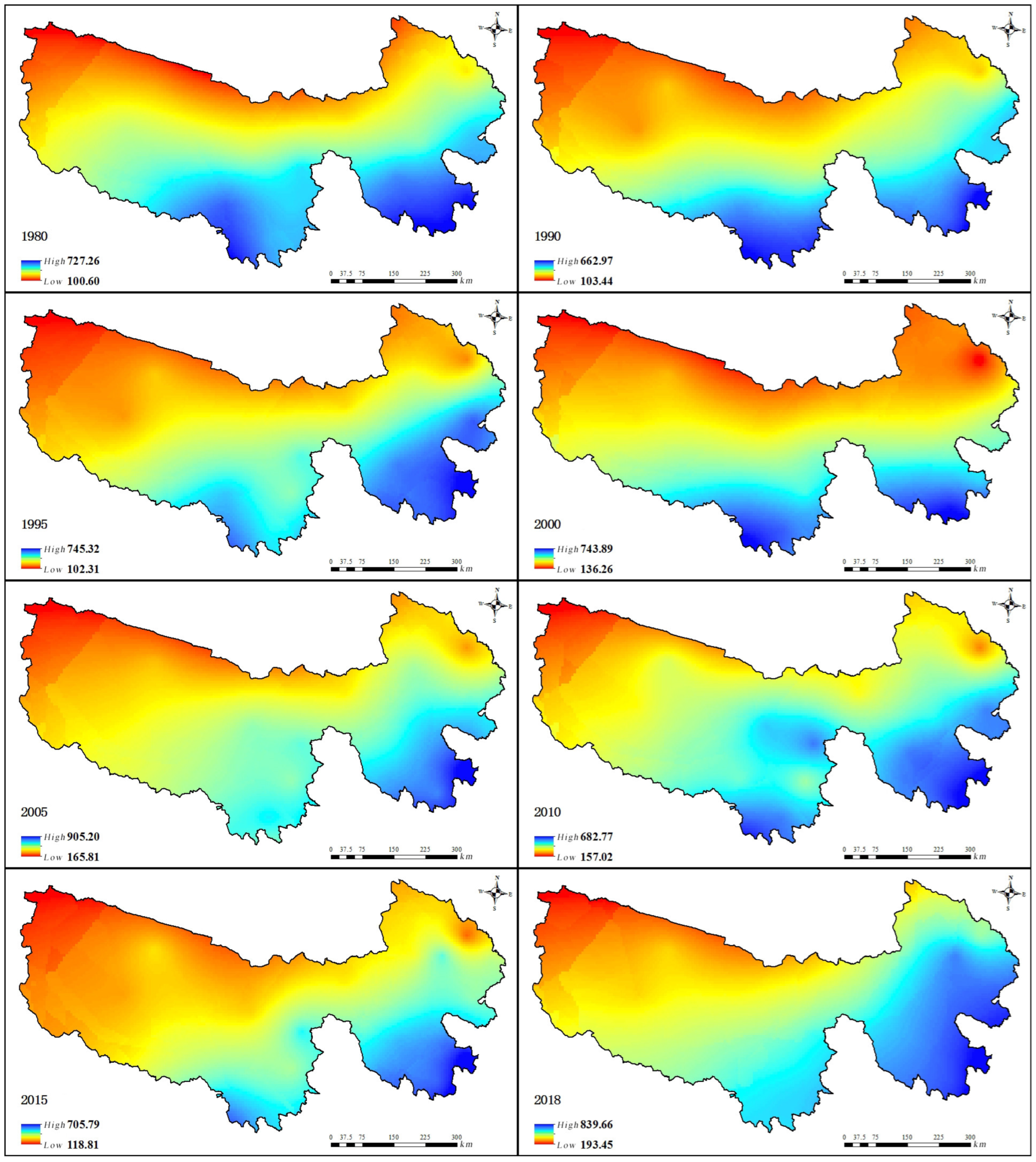
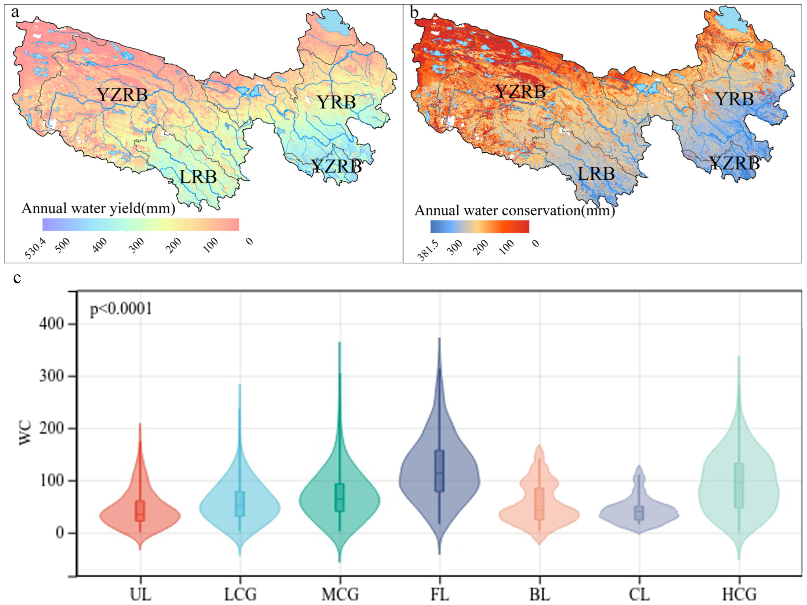
3.1.2. Simulated Results of Water Yield and Water Conservation

The average annual water yield of the TRHR from 1980 to 2018 was 137.83 mm, and the average annual WC was 50.36 mm, as shown in Figure 4. Within the respective catchment areas, the LRB led in WC, outpacing the intermediate-producing YRB and surpassing the YZRB, which recorded the minimal WC. From 1980 to 2018, the aggregate water conservation volume of the TRHR amounted to 18.933 billion cubic meters. The WC trend increased from north to south, mirroring the climatic transition from the plateau subarctic arid zone in the north to the plateau subarctic humid zone in the south (Figure 4b). The WC values by land type were as follows: Forest Land (113.36 mm), High-Coverage grassland (94.93 mm), Medium-Coverage Grassland (63.68 mm), Low-Coverage Grassland (51.59 mm), cropland (40.17 mm), Built-Up land (34.19 mm), and Unused Land (31.56 mm).

3.2. Trend Analysis of Water Conservation and Natural Factors

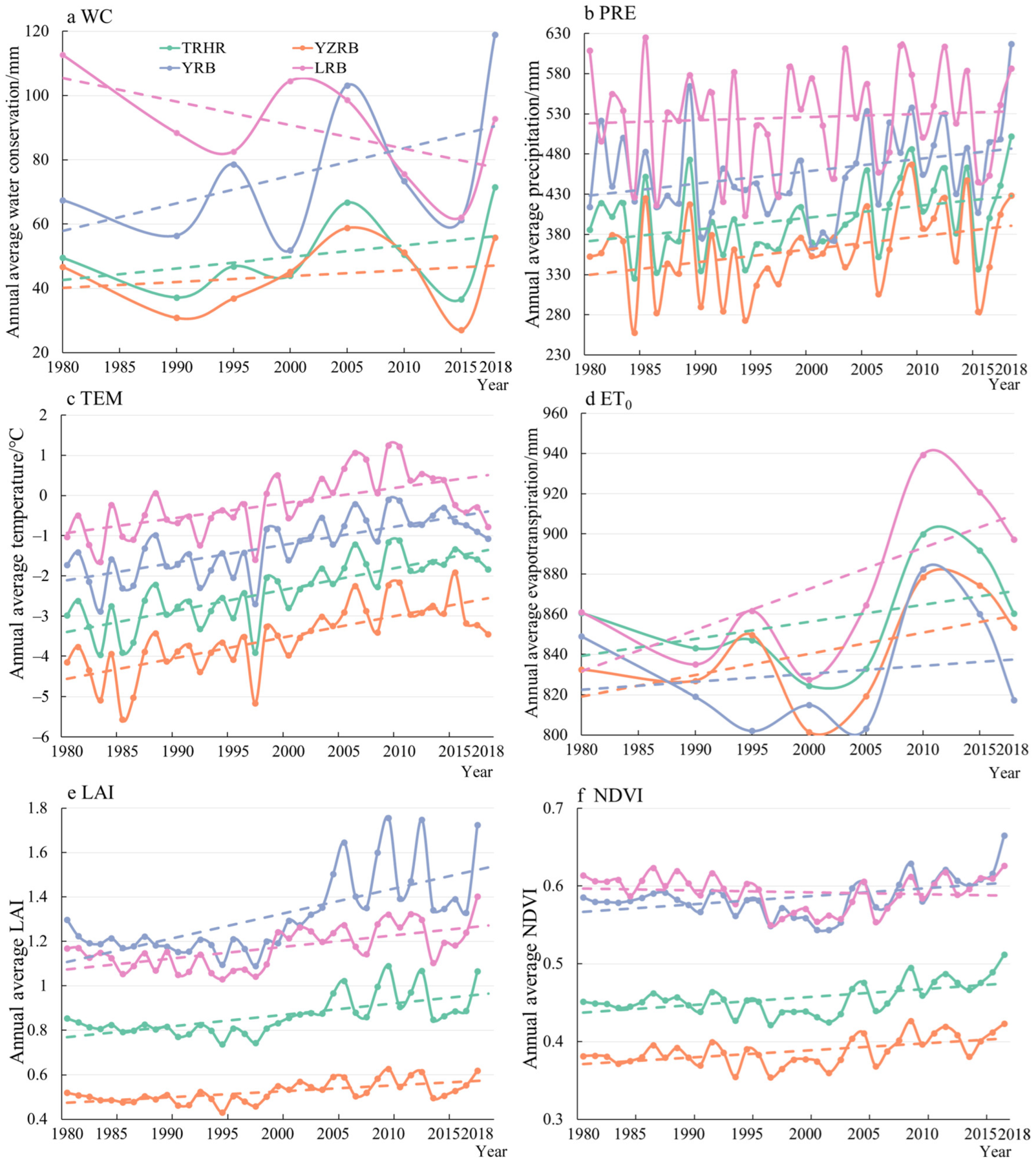
3.2.1. Trend Variation of Water Conservation and Natural Factors

The annual average WC in the TRHR demonstrated a fluctuating growth trend. Initially, in the early 1980s, the TRHR exhibited higher WC levels, which then commenced a descent, gradually elevating from 1990 onward. However, a noticeable decline was observed between 2005 and 2015, following which a significant upward trend emerged, peaking at 71.53 mm in 2018. Throughout the span of 1980–2018, the TRHR’s annual average precipitation stood at 400.03 mm, with a growth rate of 14.755 mm per decade. The alteration tendencies of precipitation and WC were notably analogous (Figure 5). The regional annual average temperature in the TRHR increased at a rate of 0.417 °C per decade, slightly surpassing the average temperature increment in global high-altitude areas. Between 2000 and 2010, a marked augmentation in ET0 was witnessed, while a slight decrement was noted during other periods, albeit the overall increase was significant. The LAI had an ascendant trajectory, with a growth rate of 0.052/10a for the 39 years. The NDVI predominantly ranged between 0.2 and 0.8, showcasing a significant upward trend post-2003 (Figure 5f).

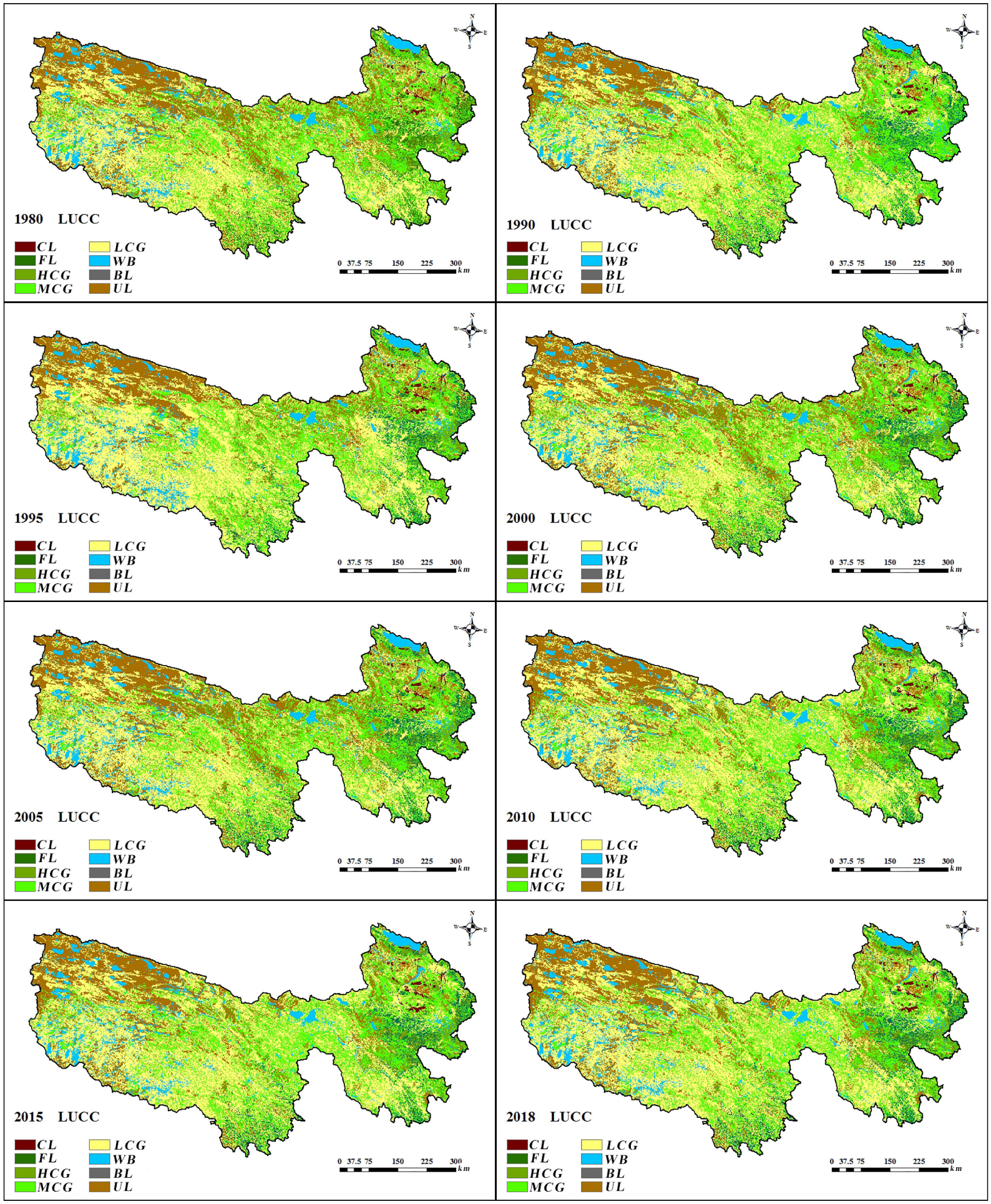
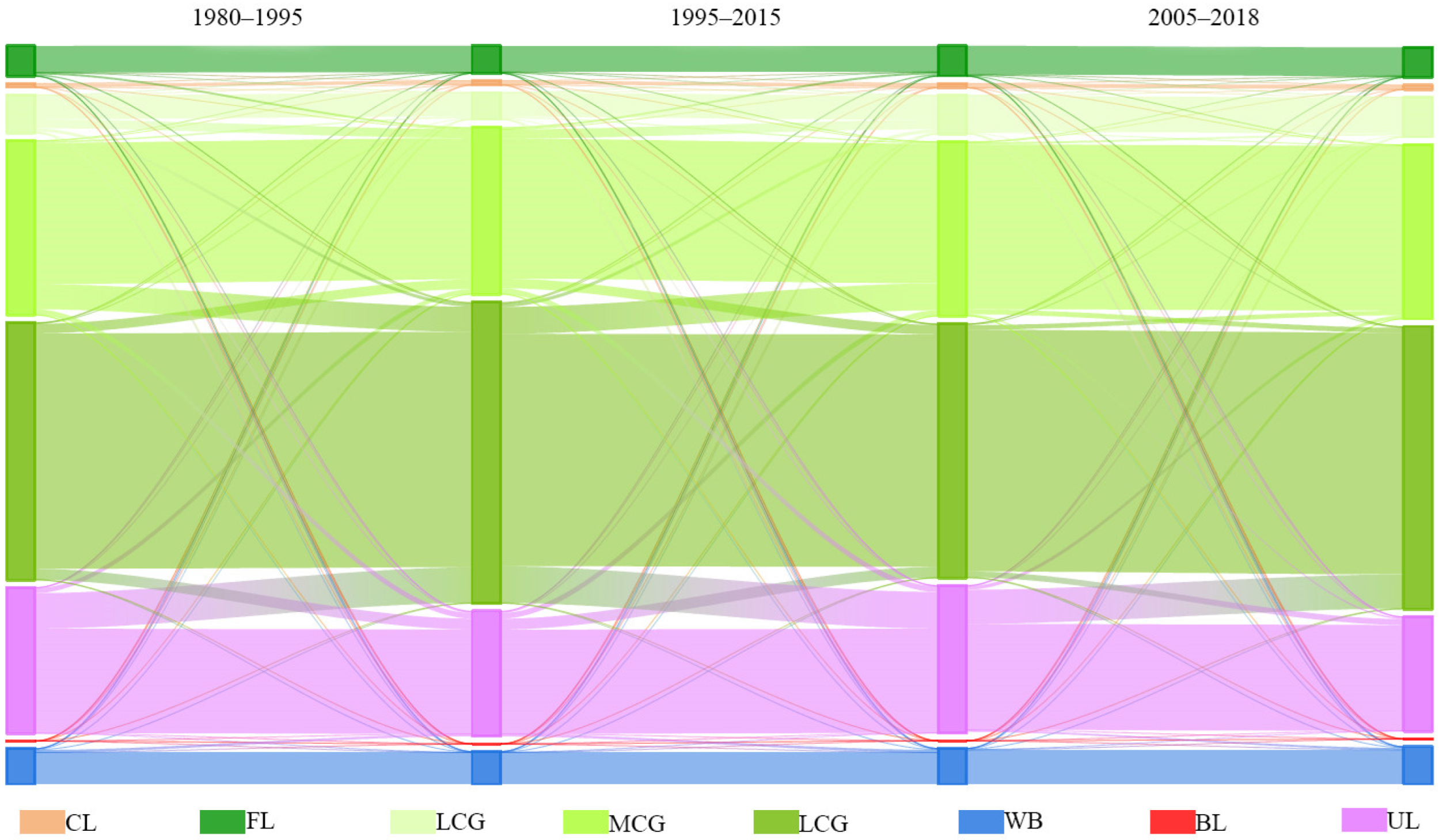
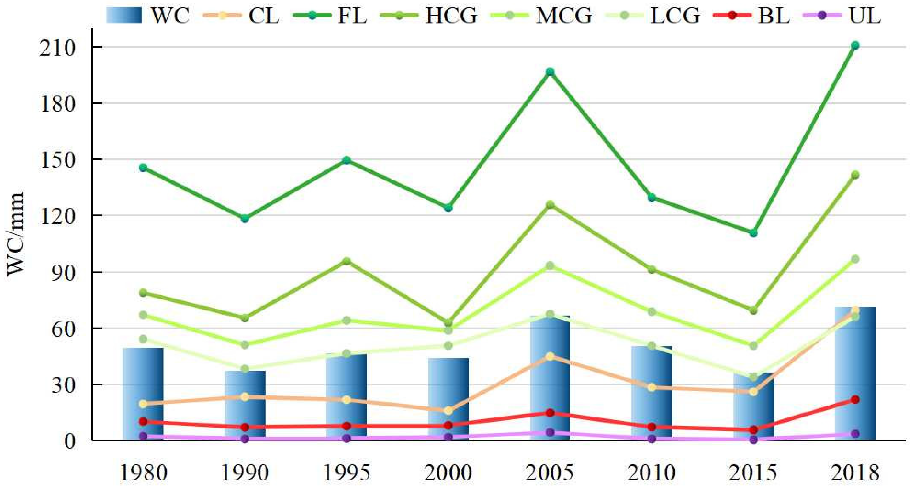
3.2.2. Fluctuations in Water Conservation across Various Land Use Types

The variations in WC among different land cover types exhibited a similar underlying trend (Figure 6 and Figure 7). FL had the most pronounced fluctuations in WC, with the magnitude of variations relative to the mean ranging from 20.06% to 42.21%. GL with high, moderate, and low vegetation cover followed, with variations in WC relative to the mean falling within the range of 24.74% to 55.01%. CL experienced comparatively smaller fluctuations, while BL and UL exhibited relatively stable WC variations. However, in all cases, the magnitude of variations in WC volume relative to the mean surpassed 100% (Figure 7) (Table 4). WC functionality was more stable in land categories characterized by thick soil layers, well-developed plant root systems, and high coverage. On the other hand, cultivated lands possessed relatively shallow root systems and soil layers that were deeply impacted by human activities, leading to lower water retention capabilities. Built-up lands and other land categories exhibited lower vegetation cover rates, with a considerably large, exposed area, hence lacking the capacity to store precipitation.
Grasslands, the predominant land use type in the TRHR (Figure 6) (Table 5), contributed significantly to WC, boasting a high per-unit area WC capacity (Figure 7). Consequently, grasslands were the primary contributors to WC in the TRHR, accounting for approximately 84.90% to 87.78% of the total WC capacity (Table 4). Although FL exhibited the highest per-unit area WC capacity, its land coverage was relatively small, contributing approximately 11.46% to 14.31% to the overall WC capacity. CL, BL, and UL contributed 0.23% to 0.68%, 0.01% to 0.02%, and 0.27% to 1.44%, respectively.

3.2.3. Mutations in Water Conservation and Natural Factors

The cumulative distance leveling method revealed that the WC underwent a mutation in approximately 2000 (Figure 8). The WC trends in the TRHR before and after the mutation point were analyzed with Theil–Sen trend analysis and the Mann–Kendall significance test. Between 1990 and 2000, the WC exhibited an overall nonsignificant rate of decrease of −1.20 mm/5a and a decrease in area of 65.57%, primarily concentrated in the YRB and LRB (Figure 8a). Conversely, from 2000 to 2018, the WC demonstrated an overall nonsignificant rate of increase of 1.75 mm/5a and an increase in area of 65.11%, mainly in the northern YRB (Figure 8b). Notably, the WC, P, TEM, ET0, LAI, and NDVI also experienced mutations from 1997–2005 (Figure 8c–h). This finding implies that abrupt alterations in climatic and vegetation factors could trigger sudden changes in WC.

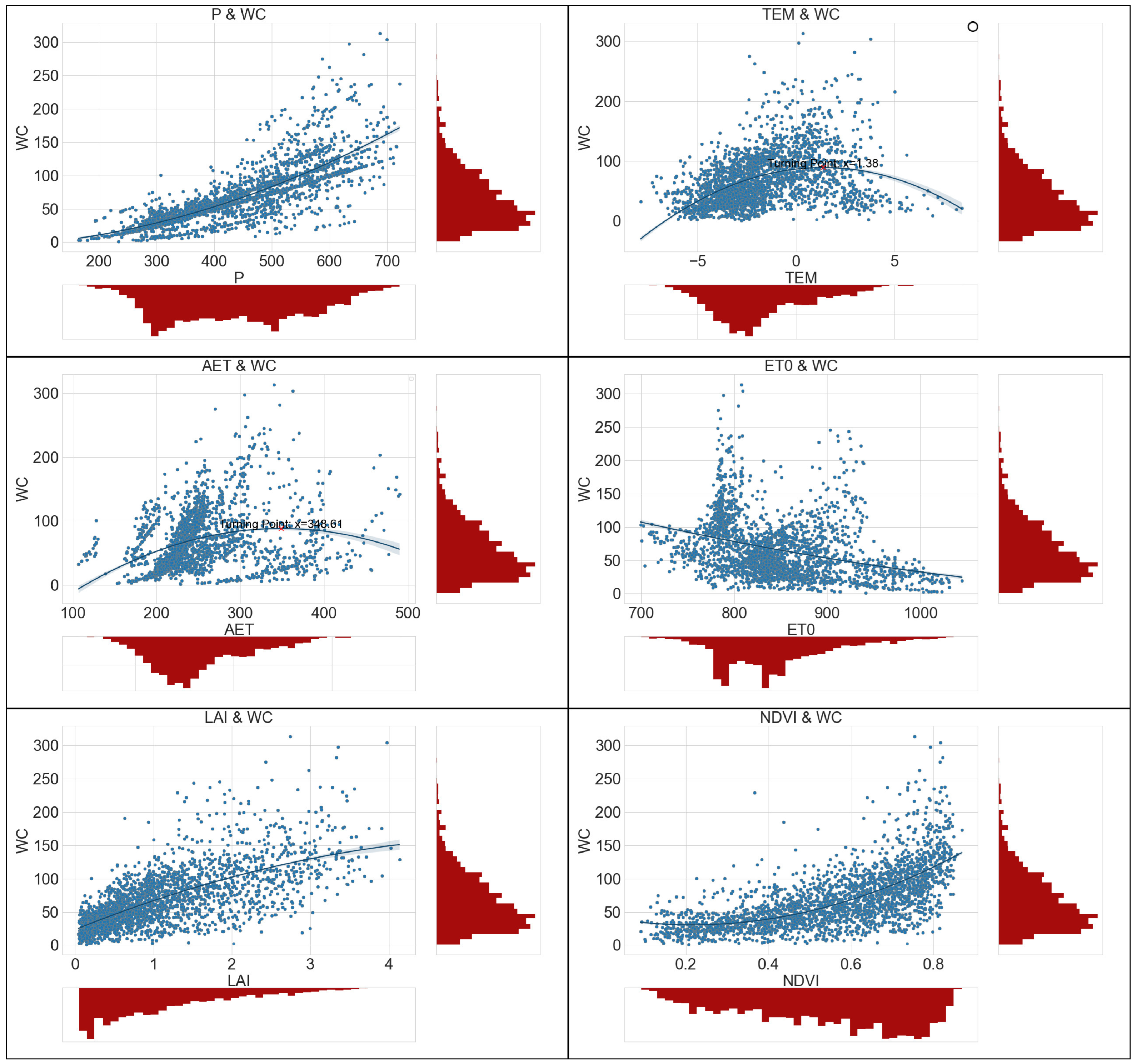
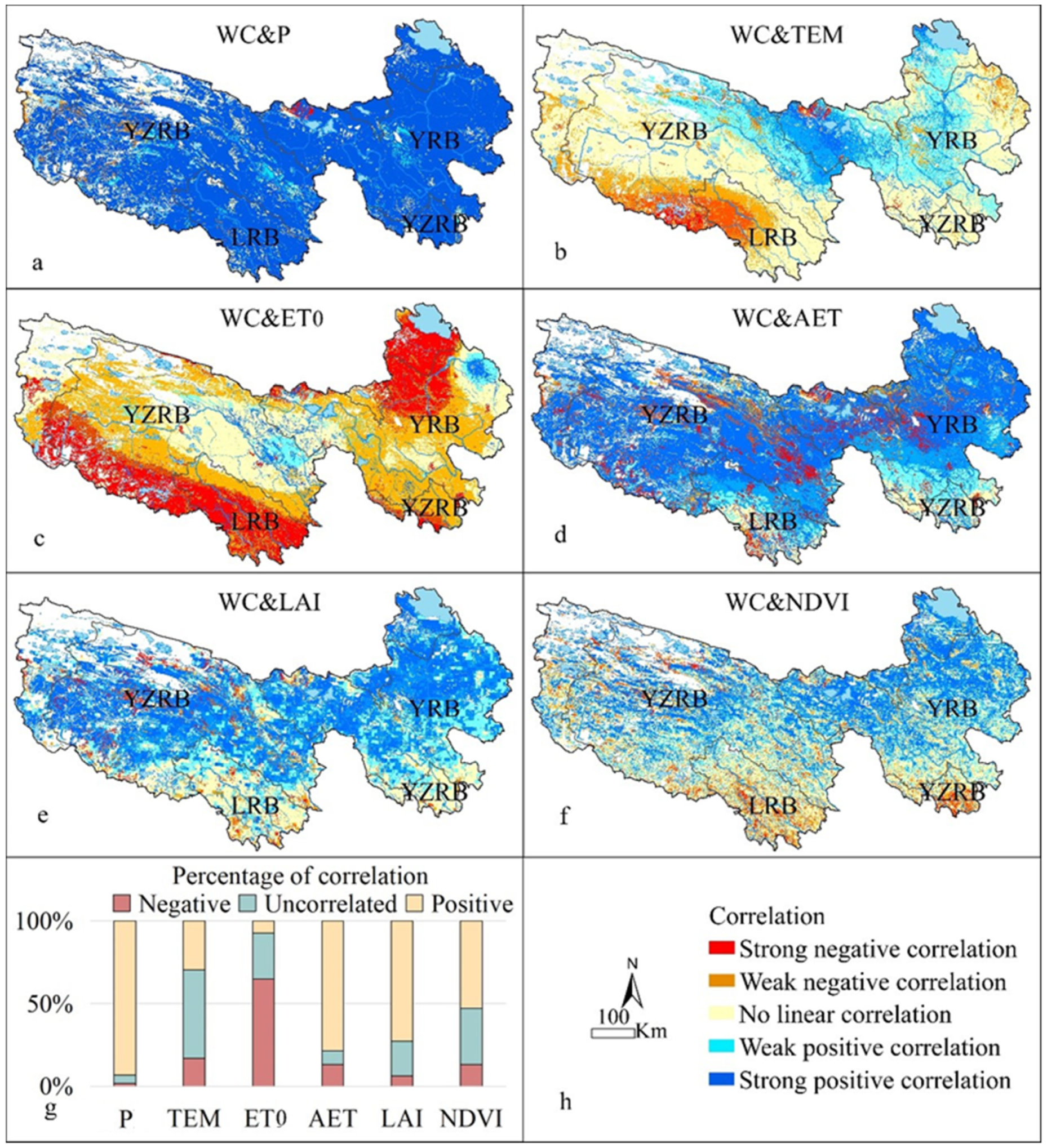
3.3. Correlation Analysis between Driving Factors and Water Conservation

Spatially, precipitation (P), temperature (TEM), actual evaporation (AET), LAI, and NDVI were positive drivers of WC, while ET0 was a negative driver of WC. The temperature in the YRB had a generally positive correlation with WC, although the response of WC to temperature varied across different regions (Figure 9b). Regions with negative correlations were concentrated in the humid area, while regions showing positive correlations were mainly concentrated in the plain and plateau landforms in the arid region with relatively low elevations. The driving effect of temperature on WC may be related to the climate zone and topography. In most areas, WC exhibited a negative correlation with reference crop evapotranspiration, which has been increasing over the past 39 years, particularly in the LRB (Figure 9c). This result indicated that the decrease in WC in the LRB was closely linked to the increase in reference crop evapotranspiration. Vegetation LAI and NDVI positively impacted WC and were predominantly distributed in the upstream and midstream areas of the YZRB and YRB (Figure 9d–f). The LAI and NDVI negatively impacted WC in the semihumid region of the southern section of the TRHR, reflecting the distinct effects of vegetation on WC in different climatic zones.
In addition to analyzing the contributions of various factors to WC, we further explored the correlations and clustering scenarios among meteorological factors, vegetation cover, and land use types with WC (Figure 10). Precipitation (P), LAI, and NDVI are highly correlated with WC (Figure 10). Concurrently, precipitation and WC are categorized together and are tightly associated with NDVI and LAI. Precipitation is a principal driver augmenting WC, whereas FRACTP and ET0 inhibit the increase in WC (Figure 10).

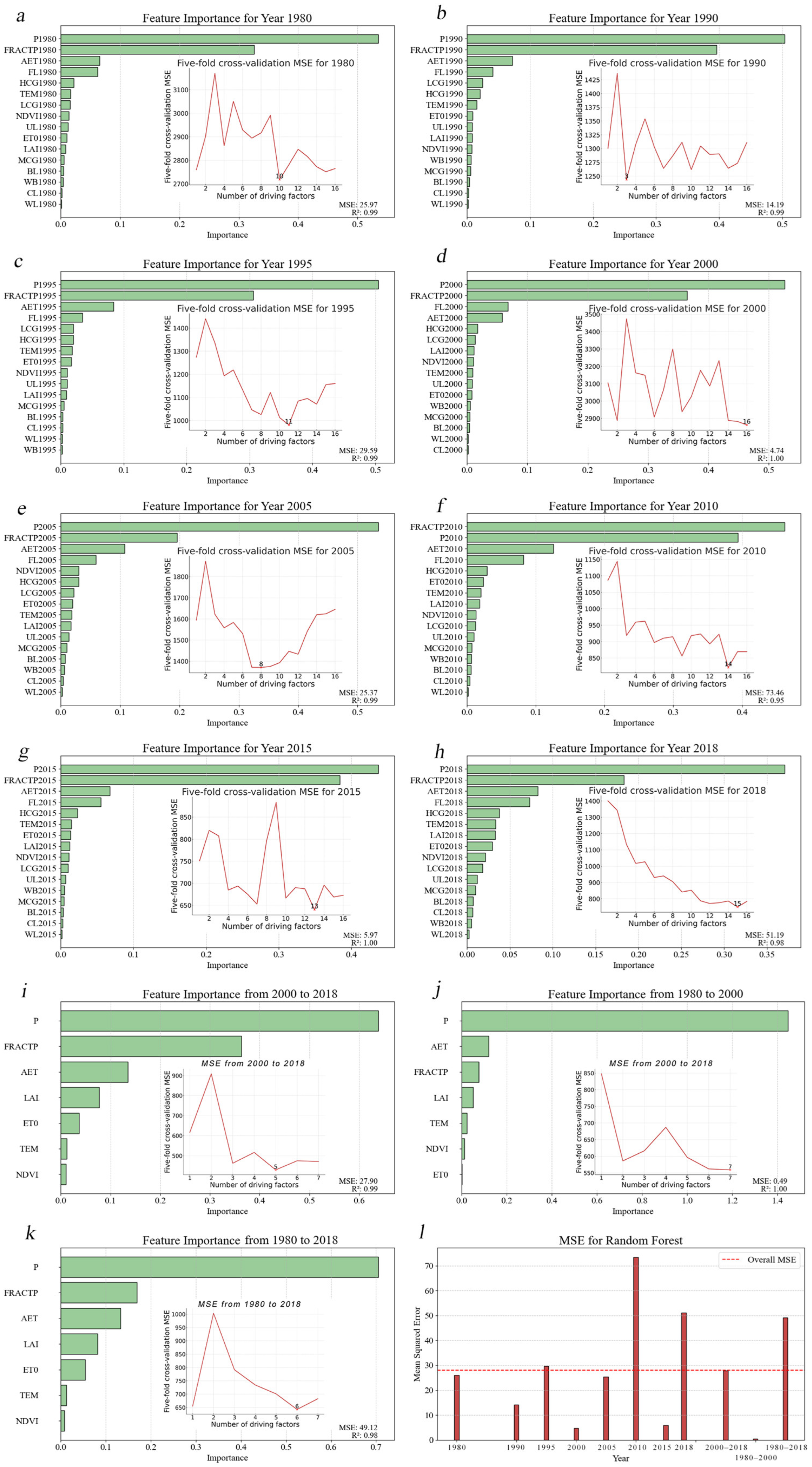
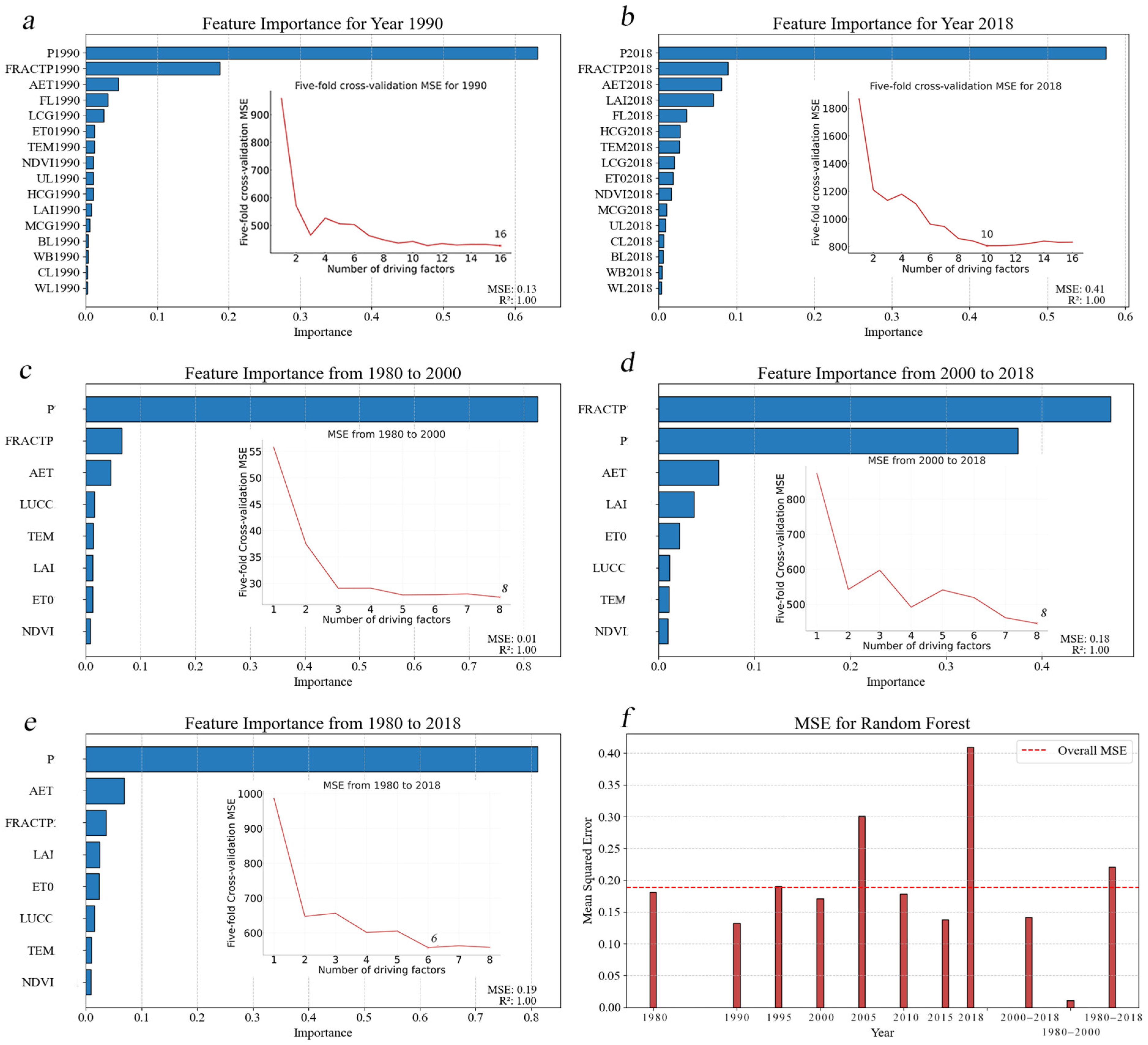
3.4. Random Forest to Assess the Importance of Each Driving Factor on Water Conservation

According to the random forest model, precipitation (P) remained the most influential variable on WC across the years, consistently ranking first in importance. Following closely was the aridity index (FRACTP) (Figure 11). The significance order of other factors tended to shift over time. Within the random forest model, AET, FL, and LAI alternately secured the third, fourth, and fifth positions, while occasionally, LCG ranked fifth importance. TEM, HCG, and ET0 maintained their standings at the sixth, seventh, and eighth, whereas UL and NDVI often occupied the ninth and tenth spots. MCG, BL, WB, CL, and WL all ranked lower, with importance values below 0.01. Disparities existed in the predictive performance of different yearly models, with the years 1990 and 2015 exhibiting better performance, whereas 2005 and 2018 showed poorer performance. The model showcased a mean squared error of 0.1887 and a high coefficient of determination R2 of 0.9999, indicating the random forest’s robust capacity for precise multiyear WC prediction (Figure 11).
The fivefold cross-validation curves revealed that as the number of considered driving factors increased, the model’s predictive performance generally increased. However, more factors do not always equate to better performance, as an excess can escalate the model’s computational complexity, possibly leading to insufficient model fitting. Additionally, substantial information overlap among selected variables may prompt model overfitting. The optimal regression point in the random forest’s fivefold cross-validation, except for the year 2000, which requires 16 indicators, necessitated only the higher-ranking importance factors for ML regression to attain the best regression outcome in other years (Figure A8).

4. Discussion

4.1. Variability in Water Conservation across Different Source Regions

The WC fluctuations in the TRHR show similarities. The LRB, being the richest in precipitation and highest in temperature among the regions, exhibits the highest WC, with a decline in fluctuations (Figure 5). The abundant precipitation, higher vegetation coverage, and predominant silty loam and loess soil textures in the LRB enhance soil water retention, contributing to its higher WC (Figure 5). These findings are consistent with those of Jian Xue et al., who observed that WC in the headwaters of the LRB surpasses that in both the Qilian Mountains and the TRHR [16]. However, it is noteworthy that, unlike our current observations, they did not report a declining trend in the WC of the LRB. Considering the relatively lower latitude of the LRB, the extent of temperature rise here is less than that in other source regions. Our spatial correlation analysis reveals that the temperature rise in the northern parts of the LRB could have adverse effects, possibly leading to a decrease in WC (Figure 9). Additionally, the ET0 in the LRB has significantly risen compared to that in the YZRB and YRB, negatively impacting WC and exacerbating the declining trend in the LRB (Figure 5). Notably, regions where WC is negatively correlated with NDVI are primarily located in the LRB (Figure 9). This specific area, characterized by shrubland and sparse forest ecosystems, is interspersed with medium- to high-coverage meadow grasslands [52,53]. Hoek van Dijke noted that due to higher canopy closure and biomass, the water consumption in these forested areas often surpasses that in other ecosystems [54]. This implies that without adequate rainfall supply, the WC function of forests could be inhibited [55,56,57,58]. Given the rapid vegetation growth in the LRB without a significant increase in precipitation, we speculate that this situation might be a key factor causing the decline in WC in this region.
The YRB exhibits the most prominent increase in WC among the three source regions (Figure 4). In contrast, the YZRB has the lowest WC and the slowest growth (Figure 5). The trend of ET0 in the YRB is not significant, implying less water consumption by the ecosystem in this region. Numerous studies have revealed that ecological protection policies such as the Grain for Green Program have progressively increased the area of grasslands and forests, protecting and restoring the desert ecosystems of the Yellow River and thereby enhancing the region’s WC [11]. This concurs with our observation that the YRB has the most significant increase in LAI and NDVI, and in most parts of the YRB, factors such as temperature and vegetation are positively correlated with WC (Figure 9). The collective alteration of these factors places the YRB at the pinnacle of the WC growth rate among the TRHR.

4.2. Analysis of the Abrupt Changes in Water Conservation

An analysis of the abrupt change nodes of WC in the TRHR in conjunction with climatic, vegetation, and land use factors discerned that WC, precipitation, temperature, evapotranspiration, LAI, and NDVI all exhibited abrupt changes between 1997 and 2005, indicating a pronounced association between these environmental factors and WC trends. Meanwhile, in 1999, China implemented the Returning Farmland to Forest and Grassland Program. In addition, all 16 indicators were needed for the five-fold cross-validation in 2000 to attain the best regression results. This situation implies that abrupt alterations in environmental factors, such as climate, vegetation, and land use changes, could trigger sudden changes in WC.
Under the influence of land use, especially after the implementation of the Returning Farmland to Forest and Grassland Program in 1999, there was a significant positive shift in land use types (29,494.44 km2) (Figure 6) (Table 5). Surprisingly, the impact on WC was not significantly enhanced. According to the ML regression results, the contribution of land use type transitions to WC ranked fourth from 1980 to 2000 but fell to sixth from 2000 to 2018 and 1980 to 2018. This finding implies that despite the positive shift in land use patterns, its impact on WC weakened over time [59], which seemingly contradicts the findings of Guanyu Jia, who observed a key promotional effect of ecological retirement projects on WC in the YRB from 2000 to 2018 [11]. Our analysis suggests that while land use change exerted some influence on WC, the abrupt alterations in climate and vegetation after 2000 had a more prominent impact. This finding does not refute the efficacy of the Returning Farmland to Forest and Grassland Program; it simply suggests that its impact might have been relatively diminished under the severe onslaught of climate and vegetation alterations.

4.3. Comprehensive Analysis of the Factors Affecting Water Conservation

Precipitation is the primary replenishment source in the TRHR, promoting vegetation growth in the TRHR, reducing soil and water loss, and thereby enhancing the WC ability of this region. Especially in this high-altitude region, a significant temperature rise leads to more snow and ice melting [60]. Although temperature elevation is conducive to plant development, potentially increasing WC, its correlation is not as pronounced as precipitation [61]. This situation may be due to the increased evapotranspiration caused by temperature rise, a process that possibly offsets the hydrological effects of glacier melting increasing WC due to temperature elevation [35,62,63]. The warming and moistening climate trend contributed to enriching the forest ecosystems of the TRHR and accelerating meadow development. With the recovery of forests and grasslands, the amount of precipitation directly hitting the ground decreases, which also weakens the impact of raindrops on the soil surface, thereby increasing soil infiltration rates [64,65] (Figure 7). Furthermore, forests can enhance vegetation root depth and improve soil organic matter and structure, rendering better conservation capacity (Figure 7) [66]. The implementation of the Grain for Green Project since 1999 has increased the coverage of grasslands and forests, enhancing the positive effects of natural factors on WC in the TRHR.
While natural factors such as precipitation promote WC, other factors such as reference crop evapotranspiration and unused land are negatively correlated with WC. In the Qinghai–Tibet Plateau region, due to strong convection or topography-induced upper-level convection, evaporation recycling is relatively active [60,67,68,69]. TEM and WB are closely positively correlated with reference crop evapotranspiration (Figure 10), and with climate warming and water body increases, their evaporation effect might be further intensified. Overall, in the context of climate warming and humidification, the execution of precise regional climate regulation and ecological protection projects are crucial for enhancing WC.

5. Conclusions

This study systematically dissected the temporal and spatial unfolding of WC within the TRHR from 1980 to 2018. A multidimensional analytical lens revealed the cardinal drivers underpinning the fluctuation in regional WC. The salient conclusions are articulated below:
(1)
The InVEST model was employed, and an average WC of 50.36 mm was computed for the TRHR during the period 1980–2018, with a total WC amounting to 189.33 billion m3, exhibiting a nonsignificant increasing trend. However, discernable disparities in WC alterations were observed among different basins. The LRB, with the highest WC, exhibited a declining fluctuation, possibly due to rapid vegetation augmentation and inconspicuous precipitation increments in this zone. Due to higher precipitation, lower potential evapotranspiration, and elevated vegetation cover, the YRB displayed the most pronounced WC augmentation.
(2)
Between 1980 and 2018, temporal junctures of abrupt environmental factor changes and abrupt WC changes were closely aligned, especially in approximately 2000, when WC transitioned from gradual diminution to noticeable augmentation. Moreover, post-2000, despite the positive transition in land use patterns, its favorable impact on WC progressively attenuated.
(3)
Precipitation emerged as the predominant driver for WC enlargement, while FRACTP and ET0 impeded WC enlargement. Grasslands made the most significant contribution to WC in the TRHR, accounting for approximately 84.90% to 87.78%.

Author Contributions

X.X. contributed to the conceptualization, data curation, investigation, formal analysis, writing original draft, and writing, review, and editing of this manuscript. M.P. contributed to data curation, resources, investigation, and writing, review, and editing. L.Z. contributed to the writing, review, and editing, project administration, and funding acquisition. M.C. contributed to the writing, review, and editing and project administration. J.L. contributed to resource management and funding acquisition. Y.T. contributed to the investigation, writing, review, and editing, and funding acquisition. All authors have read and agreed to the published version of the manuscript.

Funding

This work was supported by the National Key R&D Program of China (grant no. 2022YFC3202402), the National Key R&D Program of China (grant no. 2022YFC3202403), the National Natural Science Foundation of China (grant no. 52079083), and the Sichuan Science and Technology Program (grant no. 2021YFQ0068).

Data Availability Statement

Data are contained within the article.

Conflicts of Interest

Author Min Peng was employed by the company Gansu Province Water Resources and Hydropower Survey Design Institute Co., Ltd. The remaining authors declare that the research was conducted in the absence of any commercial or financial relationships that could be construed as a potential conflict of interest.

Appendix A. Methods

Appendix A.1. The InVEST Water Yield Model and Calculation of Water Conservation

The water yield module accounts for many factors, encompassing precipitation, evapotranspiration, land use type, and plant biophysical characteristics, with the aim of computing the water yield of every subbasin situated within a study locale [44]. The equation employed for computing the water yield is as follows:
Y i e l d ( x ) = 1 A E T ( x ) P ( x ) × P ( x )
where Y i e l d ( x ) represents the water yield, A E T ( x ) denotes the actual annual evapotranspiration, and P ( x ) denotes the annual precipitation in mm.
The vegetation evapotranspiration of land use types, A E T ( x ) / P ( x ) , was computed by employing the Budyko water–heat coupled equilibrium assumption formula suggested by Fu et al. [70]. P E T ( x ) represents the potential evapotranspiration in millimeters, and ω ( x ) denotes a nonphysical parameter that characterizes the combined climate and soil properties [71]. P E T ( x ) denotes the prospective evapotranspiration, as defined by the following equation:
A E T ( x ) P ( x ) = 1 + P E T ( x ) P ( x ) 1 + P E T ( x ) P ( x ) ω ( x ) 1 ω ( x )
P E T ( x ) = k c ( l x ) E T 0 ( x )
k c ( l x ) = L A I 3 ( L A I 3 ) 1 ( L A I > 3 )
where ET0 is the reference crop evapotranspiration in mm. The evapotranspiration coefficient of various land use types is denoted by k c ( l x ) , and L A I is the mean Leaf Area Index of the growing season, defined as the monthly average of the Leaf Area Index during May–September.
ω ( x ) in the InVEST model is computed using the empirical equation suggested by Donohue:
ω ( x ) = Z A W C ( x ) P ( x ) + 1.25
where Z represents the Zhang empirical coefficient, and A W C ( x ) denotes the effective soil water content in mm, determined by the minimum values of plant available water content (PAWC), maximum soil root burial depth ( r e s t . l a y e r . d e p t h ), and plant root depth ( r o o t . d e p t h ), calculated as follows:
A W C ( x ) = min ( r e s t . l a y e r . d e p t h , r o o t . d e p t h ) × P A W C
P A W C = 54.509 0.132 s a n d 0.003 s a n d 2 0.055 s i l t 0.006 s i l t 2 0.738 c l a y + 0.007 c l a y 2 2.688 O M + 0.501 O M 2
This study calculated the daily ET0 value in the TRHR using the Penman–Monteith formula and accumulated it to obtain the annual reference crop evapotranspiration [72,73]. The particular formula is delineated as follows:
E T 0 = 0.408 Δ ( R n G ) + γ 900 T m e a n + 273 u 2 ( e s e a ) Δ + γ ( 1 + 0.34 u 2 )
where ET0 denotes the day-by-day potential evapotranspiration, Δ denotes the slope of the saturation water vapor pressure curve, G denotes the soil heat flux, R n denotes the net surface radiation, T m e a n denotes the average daily temperature at a height of 2 m, γ denotes the wet and dry gauge constants, u 2 denotes the wind speed at a 2 m height, e s denotes the saturation water pressure, and e a denotes the actual water vapor pressure.

Appendix A.2. M-K Mutation Detection Methods

The M-K mutation detection method is articulated through the following computational steps:
Initially, construct a statistic for the sequence x i , t = 1 , 2 , , m ( m n ) . Secondly, set m = 1 , 2 , , n , compute the statistic U d m , and plot. At this juncture, U d m  (when m is fixed) asymptotically follows the N(0, 1) distribution. Thirdly, reverse the sequence x i to form the sequence x t , repeat the preceding two steps to obtain the statistic U d m , and set U d m = U d m , m = n m + 1 . Lastly, plot U d m and U d m on the same graph, identify the intersection of the two lines, and if the U value at this point satisfies U < 1.96 , the hypothesis of a mutation point can be accepted with a test confidence level of α = 0.05
d m = i = 1 m j = 1 i 1 r i j
U ( d m ) = [ d m E ( d m ) ] / V a r ( d m )
E ( d m ) = m ( m 1 ) / 4
V a r ( d m ) = m ( m 1 ) ( 2 m + 5 ) / 72

Appendix A.3. Land Use Transfer Matrix

The land use transfer matrix was used to scrutinize the spatial distribution and mutual transfer features of discrete land categories in the TRHR in each phase [74]. This model is primarily presented in the form of a two-dimensional matrix, and its mathematical representation is as follows:
S i j = S 11 S 1 n S n 1 S n n
where S i j represents the region where the ith land use category has been converted into the jth land use category, and when i = j , it refers to the area that has not undergone any transformation itself, measured in km2. Moreover, the parameter n presents the number of distinct land use categories in the TRHR.
Table A1. Land use types after reclassification in the TRHR.
No.Land Use TypeDescription
1Cropland (CL)Refers to paddy fields as no dry lands were found in the study area.
2Forest Land (FL)Encompasses forested areas, shrublands, sparse forests, and other forms of woodland.
3High-Coverage Grassland (HCG)Denotes natural grasslands, mowed grasslands, and improved grasslands with vegetation cover exceeding 50%.
4Medium-Coverage Grassland (MCG)Refers to natural and improved grasslands with vegetation cover ranging from 20% to 50%.
5Low-Coverage Grassland (LCG)Refers to natural grasslands with vegetation cover ranging from 5% to 20%.
6Water Bodies (WB)Refers to natural terrestrial waters and hydraulic facilities, mainly including rivers, lakes, beaches, reservoirs, and permanent glaciers and snowfields.
7Built-up Land (BL)Refers to land used for urban and rural residential areas, as well as other built-up areas such as industrial parks and transportation facilities.
8Unused Land (UL)Refers to land that is not currently used, including sandy, desert, saline–alkali, bare, rocky, swampy, and other unusable land, such as high-altitude deserts and tundras.
9Wetland (WL)Wetlands, characterized by low-lying areas inundated with water, are teeming with diverse vegetation and extensive mudflats.

Appendix A.4. Fitting between the Scatter of Natural Factors and Water Conservation

A second-order regression of scatter plots was conducted on the mean values of each natural factor from 1980 to 2018, subsequently producing marginal histograms. The quadratic regression curves of precipitation and NDVI regarding water conservation show a similar concave growth trend. This indicates that as precipitation and NDVI increase, the rate of increase in WC accelerates. Meanwhile, as the Leaf Area Index (LAI) rises, the increase in WC tends to level off. With increasing temperatures, WC initially rises, peaking at 1.38 °C, after which it begins to decline. The trends for Actual Evapotranspiration (AET) mirror those of temperature, exhibiting a turning point at 384.84 mm. The scatter points of the six natural factors were more dispersed around the fitted curves, suggesting that there is a great deal of variability in the relationship between the factors and the WC, and that the relationships need to be further explored.
Figure A1. A second-order polynomial regression between natural factors and water conservation. The scatterplot visualizes the relationship, highlighting the turning point with a red ‘x’. Marginal histograms offer distributions of natural factors and water conservation.
Land 13 00352 g0a1

Appendix B. Establishment of the InVEST Model

The data inputs for the InVEST model encompass annual precipitation, annual reference crop evapotranspiration, soil depth, available water content in vegetation, land use types, a biophysical coefficient table containing parameters such as evapotranspiration coefficients for different land classes and root depths for various vegetation types, as well as vector boundaries for basins and subbasins.
Figure A2. Spatial distribution of precipitation in the TRHR from 1980 to 2018.
Land 13 00352 g0a2
Figure A3. Spatial distribution of temperature in the TRHR from 1980 to 2018.
Land 13 00352 g0a3
Figure A4. Spatial distribution of land use or cover categories in the TRHR from 1980 to 2018.
Land 13 00352 g0a4
Figure A5. Soil properties.
Land 13 00352 g0a5
Figure A6. The average annual water yield distribution from 1980 to 2018 in the TRHR. (ah) are the average annual water yield distribution of 1980, 1990, 1995, 2000, 2005, 2010, 2015 and 2018, respectively.
Land 13 00352 g0a6
Figure A7. Distribution of average annual water conservation from 1980 to 2018 in the TRHR. (ah) are the distribution of average annual water conservation in 1980, 1990, 1995, 2000, 2005, 2010, 2015 and 2018, respectively.
Land 13 00352 g0a7
Figure A8. The importance and MSE of feature by the random forest in different years. (ak) represent the feature importance in 1980, 1990, 1995, 2000, 2005, 2010, 2015, 2018, 2000–2018, 1980–2000 and 1980–2018, respectively. (l) is the MSE for Random Forest.
Land 13 00352 g0a8
Figure A9. The importance and MSE of feature by the XGBoost in different years. (ak) represent the feature importance in 1980, 1990, 1995, 2000, 2005, 2010, 2015, 2018, 2000–2018, 1980–2000 and 1980–2018, respectively. (l) is the MSE for XGBoost.
Land 13 00352 g0a9
Figure A10. Cluster analysis and correlation analysis of the main drivers of water conservation in different years. (ah) represent the analysis results in 1980, 1990, 1995, 2000, 2005, 2010, 2015 and 2018, respectively.
Land 13 00352 g0a10
Table A2. Abbreviations and Symbols.
Abbreviations and SymbolsMeaningsUnits
AETActual Evapotranspirationmm
AWCEffective soil water contentmm
BLBuilt-up Land-
CDACumulative distance adjustment-
CLCropland-
DEMDigital Elevation Model-
esActual water vapor pressurekPa
ET0Reference Crop Evapotranspirationmm
FLForest Land-
FRACTPAridity Index-
GSoil heat fluxMJ·m−2·d−1
HCGHigh-Coverage Grassland-
IncMSEIncremental mean squared errorconsistent with element units
KcActual crop coefficient-
KsSaturated hydraulic conductivitycm/d
LAILeaf Area Index-
LCGLow-Coverage Grassland-
LiCumulative distance from mean valueconsistent with element units
LRBLancang River Basin-
LUCCLand use and cover changekm2
MCGMedium-Coverage Grassland-
M-KMann–Kendall-
MLMachine Learning-
NDVINormalized Difference Vegetation Index-
OMOrganic matter content in soil%
PAnnual Precipitationmm
PAWCMinimum values of plant available water contentmm
PETPotential evapotranspirationmm
rPearson correlation coefficient-
R ¯ Multiyear average of the elementconsistent with element units
RFRandom forest-
RiElement value of the ith yearconsistent with element units
RnNet surface radiationMJ·m−2·d−1
SijRegion where the ith land use category has been converted into the jth land use category-
TmeanAverage daily temperature at a height of 2 m°C
TEMAverage Annual Temperature°C
TIDimensionless topographic index-
TRHRThree-River Headstreams Region-
u2Wind speed at a 2 m heightm/s
ULUnused Land-
VelocityFlow rate coefficient-
WBWater Bodies-
WCWater conservationmm
WLWetland-
YieldWater yieldmm
YRBYellow River Basin-
YZRBYangtze River Basin-
ZZhang empirical coefficient-
αCatchment area per unit contour length at any point of the flow through the slopekm2
βSlope angle°
γWet and dry gauge constantskPa/°C
ω Plant-available water coefficient-
Slope of the saturation water vapor pressure curvekPa/°C

References

  1. Ali, D.A.; Deininger, K.; Monchuk, D. Using satellite imagery to assess impacts of soil and water conservation measures: Evidence from Ethiopia’s Tana-Beles watershed. Ecol. Econ. 2020, 169, 106512. [Google Scholar] [CrossRef]
  2. Bonell, M. Progress in the understanding of runoff generation dynamics in forests. J. Hydrol. 1993, 150, 217–275. [Google Scholar] [CrossRef]
  3. Costanza, R.; D’Arge, R.; De Groot, R.; Farber, S.; Grasso, M.; Hannon, B.; Limburg, K.; Naeem, S.; O’Neill, R.V.; Paruelo, J.; et al. The value of the world’s ecosystem services and natural capital. Ecol. Econ. 1998, 25, 3–15. [Google Scholar] [CrossRef]
  4. Baker, T.J.; Miller, S.N. Using the Soil and Water Assessment Tool (SWAT) to assess land use impact on water resources in an East African watershed. J. Hydrol. 2013, 486, 100–111. [Google Scholar] [CrossRef]
  5. Benra, F.; De Frutos, A.; Gaglio, M.; Álvarez-Garretón, C.; Felipe-Lucia, M.; Bonn, A. Mapping water ecosystem services: Evaluating InVEST model predictions in data scarce regions. Environ. Model. Softw. 2021, 138, 104982. [Google Scholar] [CrossRef]
  6. Chen, J.M.; Chen, X.; Ju, W.; Geng, X. Distributed hydrological model for mapping evapotranspiration using remote sensing inputs. J. Hydrol. 2005, 305, 15–39. [Google Scholar] [CrossRef]
  7. Goldstein, J.H.; Caldarone, G.; Duarte, T.K.; Ennaanay, D.; Hannahs, N.; Mendoza, G.; Polasky, S.; Wolny, S.; Daily, G.C. Integrating ecosystem-service tradeoffs into land-use decisions. Proc. Natl. Acad. Sci. USA 2012, 109, 7565–7570. [Google Scholar] [CrossRef]
  8. Hamel, P.; Chaplin-Kramer, R.; Sim, S.; Mueller, C. A new approach to modeling the sediment retention service (InVEST 3.0): Case study of the Cape Fear catchment, North Carolina, USA. Sci. Total Environ. 2015, 524–525, 166–177. [Google Scholar] [CrossRef] [PubMed]
  9. Redhead, J.; Stratford, C.; Sharps, K.; Jones, L.; Ziv, G.; Clarke, D.; Oliver, T.; Bullock, J. Empirical validation of the InVEST water yield ecosystem service model at a national scale. Sci. Total Environ. 2016, 569–570, 1418–1426. [Google Scholar] [CrossRef]
  10. Pessacg, N.; Flaherty, S.; Brandizi, L.; Solman, S.; Pascual, M. Getting water right: A case study in water yield modelling based on precipitation data. Sci. Total Environ. 2015, 537, 225–234. [Google Scholar] [CrossRef]
  11. Jia, G.; Hu, W.; Zhang, B.; Li, G.; Shen, S.; Gao, Z.; Li, Y. Assessing impacts of the Ecological Retreat project on water conservation in the Yellow River Basin. Sci. Total Environ. 2022, 828, 154483. [Google Scholar] [CrossRef] [PubMed]
  12. Wu, C.; Qiu, D.; Gao, P.; Mu, X.; Zhao, G. Application of the InVEST model for assessing water yield and its response to precipitation and land use in the Weihe River Basin, China. J. Arid Land 2022, 14, 426–440. [Google Scholar] [CrossRef]
  13. Yang, J.; Xie, B.; Zhang, D.; Tao, W. Climate and land use change impacts on water yield ecosystem service in the Yellow River Basin, China. Environ. Earth Sci. 2021, 80, 72. [Google Scholar] [CrossRef]
  14. Wang, J.; Wu, T.; Li, Q.; Wang, S. Quantifying the effect of environmental drivers on water conservation variation in the eastern Loess Plateau, China. Ecol. Indic. 2021, 125, 107493. [Google Scholar] [CrossRef]
  15. Wang, Y.; Ye, A.; Peng, D.; Miao, C.; Di, Z.; Gong, W. Spatiotemporal variations in water conservation function of the Tibetan Plateau under climate change based on InVEST model. J. Hydrol. Reg. Stud. 2022, 41, 101064. [Google Scholar] [CrossRef]
  16. Xue, J.; Li, Z.; Feng, Q.; Gui, J.; Zhang, B. Spatiotemporal variations of water conservation and its influencing factors in ecological barrier region, Qinghai-Tibet Plateau. J. Hydrol. Reg. Stud. 2022, 42, 101164. [Google Scholar] [CrossRef]
  17. Bi, Y.; Zheng, L.; Wang, Y.; Li, J.; Yang, H.; Zhang, B. Coupling relationship between urbanization and water-related ecosystem services in China’s Yangtze River economic Belt and its socio-ecological driving forces: A county-level perspective. Ecol. Indic. 2023, 146, 109871. [Google Scholar] [CrossRef]
  18. Li, M.; Liang, D.; Xia, J.; Song, J.; Cheng, D.; Wu, J.; Cao, Y.; Sun, H.; Li, Q. Evaluation of water conservation function of Danjiang River Basin in Qinling Mountains, China based on InVEST model. J. Environ. Manag. 2021, 286, 112212. [Google Scholar] [CrossRef]
  19. Chen, Q.; Xu, X.; Wu, M.; Wen, J.; Zou, J. Assessing the Water Conservation Function Based on the InVEST Model: Taking Poyang Lake Region as an Example. Land 2022, 11, 2228. [Google Scholar] [CrossRef]
  20. Hu, W.; Li, G.; Li, Z. Spatial and temporal evolution characteristics of the water conservation function and its driving factors in regional lake wetlands—Two types of homogeneous lakes as examples. Ecol. Indic. 2021, 130, 108069. [Google Scholar] [CrossRef]
  21. Wang, X.; Liu, L.; Zhang, S.; Gao, C. Dynamic simulation and comprehensive evaluation of the water resources carrying capacity in Guangzhou city, China. Ecol. Indic. 2022, 135, 108528. [Google Scholar] [CrossRef]
  22. Yin, L.; Dai, E.; Guan, M.; Zhang, B. A novel approach for the identification of conservation priority areas in mountainous regions based on balancing multiple ecosystem services—A case study in the Hengduan Mountain region. Glob. Ecol. Conserv. 2022, 38, e02195. [Google Scholar] [CrossRef]
  23. Cheng, L.; Chen, X.; De Vos, J.; Lai, X.; Witlox, F. Applying a random forest method approach to model travel mode choice behavior. Travel Behav. Soc. 2019, 14, 1–10. [Google Scholar] [CrossRef]
  24. Bagheri, M.; Farshforoush, N.; Bagheri, K.; Shemirani, A.I. Applications of artificial intelligence technologies in water environments: From basic techniques to novel tiny machine learning systems. Process. Saf. Environ. Prot. 2023, 180, 10–22. [Google Scholar] [CrossRef]
  25. Li, Z.; Wang, W.; Ji, X.; Wu, P.; Zhuo, L. Machine learning modeling of water footprint in crop production distinguishing water supply and irrigation method scenarios. J. Hydrol. 2023, 625, 130171. [Google Scholar] [CrossRef]
  26. Lu, Y.; Tuo, Y.; Xia, H.; Zhang, L.; Chen, M.; Li, J. Prediction model of the outflow temperature from stratified reservoir regulated by stratified water intake facility based on machine learning algorithm. Ecol. Indic. 2023, 154, 110560. [Google Scholar] [CrossRef]
  27. Li, S.; Yu, D.; Huang, T.; Hao, R. Identifying priority conservation areas based on comprehensive consideration of biodiversity and ecosystem services in the Three-River Headwaters Region, China. J. Clean. Prod. 2022, 359, 132082. [Google Scholar] [CrossRef]
  28. Ma, T.; Swallow, B.; Foggin, J.M.; Zhong, L.; Sang, W. Co-management for sustainable development and conservation in Sanjiangyuan National Park and the surrounding Tibetan nomadic pastoralist areas. Humanit. Soc. Sci. Commun. 2023, 10, 321. [Google Scholar] [CrossRef]
  29. Shao, Q.; Cao, W.; Fan, J.; Huang, L.; Xu, X. Effects of an ecological conservation and restoration project in the Three-River Source Region, China. J. Geogr. Sci. 2017, 27, 183–204. [Google Scholar] [CrossRef]
  30. Ahmed, N.; Wang, G.; Booij, M.J.; Oluwafemi, A.; Hashmi, M.Z.-U.; Ali, S.; Munir, S. Climatic Variability and Periodicity for Upstream Sub-Basins of the Yangtze River, China. Water 2020, 12, 842. [Google Scholar] [CrossRef]
  31. Pan, Y.; Yin, Y. Spatial and Temporal Evolution Characteristics of Water Conservation in the Three-Rivers Headwater Region and the Driving Factors over the Past 30 Years. Atmosphere 2023, 14, 1453. [Google Scholar] [CrossRef]
  32. Yuan, X.; Wang, W.; Cui, J.; Meng, F.; Kurban, A.; De Maeyer, P. Vegetation changes and land surface feedbacks drive shifts in local temperatures over Central Asia. Sci. Rep. 2017, 7, 3287. [Google Scholar] [CrossRef]
  33. Cominola, A.; Giuliani, M.; Castelletti, A.; Fraternali, P.; Gonzalez, S.L.H.; Herrero, J.C.G.; Novak, J.; Rizzoli, A.E. Long-term water conservation is fostered by smart meter-based feedback and digital user engagement. NPJ Clean Water 2021, 4, 29. [Google Scholar] [CrossRef]
  34. Liu, D.; Cao, C.; Dubovyk, O.; Tian, R.; Chen, W.; Zhuang, Q.; Zhao, Y.; Menz, G. Using fuzzy analytic hierarchy process for spatio-temporal analysis of eco-environmental vulnerability change during 1990–2010 in Sanjiangyuan region, China. Ecol. Indic. 2017, 73, 612–625. [Google Scholar] [CrossRef]
  35. Li, Z.; Li, Z.; Qi, F.; Wang, X.; Mu, Y.; Xin, H.; Song, L.; Juan, G.; Zhang, B.; Gao, W.; et al. Hydrological effects of multiphase water transformation in Three-River Headwaters Region, China. J. Hydrol. 2021, 601, 126662. [Google Scholar] [CrossRef]
  36. Li, Y.; Li, B.; Yuan, Y.; Lei, Q.; Jiang, Y.; Liu, Y.; Li, R.; Liu, W.; Zhai, D.; Xu, J. Trends in total nitrogen concentrations in the Three Rivers Headwater Region. Sci. Total. Environ. 2022, 852, 158462. [Google Scholar] [CrossRef] [PubMed]
  37. Lv, L.-S.; Jin, D.-H.; Ma, W.-J.; Liu, T.; Xu, Y.-Q.; Zhang, X.-E.; Zhou, C.-L. The Impact of Non-optimum Ambient Temperature on Years of Life Lost: A Multi-county Observational Study in Hunan, China. Int. J. Environ. Res. Public Health 2020, 17, 2699. [Google Scholar] [CrossRef] [PubMed]
  38. Shangguan, W.; Dai, Y. A China Soil Characteristics Dataset (2010); National Tibetan Plateau/Third Pole Environment Data Center: Lhasa, China, 2023. [Google Scholar] [CrossRef]
  39. Fan, X.; Wang, L.; Li, X.; Zhou, J.; Chen, D.; Yang, H. Increased discharge across the Yellow River Basin in the 21st century was dominated by precipitation in the headwater region. J. Hydrol. Reg. Stud. 2022, 44, 101230. [Google Scholar] [CrossRef]
  40. Liu, Y.; Liu, R.; Chen, J.M. Retrospective retrieval of long-term consistent global leaf area index (1981–2011) from combined AVHRR and MODIS data. J. Geophys. Res. Biogeosci. 2012, 117, G04003. [Google Scholar] [CrossRef]
  41. Piao, S.; Fang, J.; Zhou, L.; Ciais, P.; Zhu, B. Variations in Satellite-Derived Phenology in China’s Temperate Vegetation. Glob. Change Biol. 2006, 12, 672–685. [Google Scholar] [CrossRef]
  42. Nascimento, C.M.; Mendes, W.d.S.; Silvero, N.E.Q.; Poppiel, R.R.; Sayão, V.M.; Dotto, A.C.; dos Santos, N.V.; Amorim, M.T.A.; Demattê, J.A. Soil degradation index developed by multitemporal remote sensing images, climate variables, terrain and soil atributes. J. Environ. Manag. 2021, 277, 111316. [Google Scholar] [CrossRef] [PubMed]
  43. Negash, T.W.; Bayisa, G.D.; Tefera, A.T.; Bizuneh, K.T.; Dinku, A.G.; Awulachew, T.W.; Bikela, G.A. Evapotranspiration and crop coefficient of sorghum (Sorghum bicolor L.) at melkassa farmland, semi-arid area of ethiopia. Air Soil Water Res. 2023, 16, 11786221231184206. [Google Scholar] [CrossRef]
  44. Minga-León, S.; Gómez-Albores, M.A.; Bâ, K.M.; Balcázar, L.; Manzano-Solís, L.R.; Cuervo-Robayo, A.P.; Mastachi-Loza, C.A. Estimation of water yield in the hydrographic basins of southern Ecuador. Hydrol. Earth Syst. Sci. Discuss. 2018, 1–18. [Google Scholar] [CrossRef]
  45. Liu, Y.; Li, Z.; Chen, Y.; Li, Y.; Li, H.; Xia, Q.; Kayumba, P.M. Evaluation of consistency among three NDVI products applied to High Mountain Asia in 2000–2015. Remote Sens. Environ. 2022, 269, 112821. [Google Scholar] [CrossRef]
  46. Xu, H.-J.; Zhao, C.-Y.; Wang, X.-P.; Chen, S.-Y.; Shan, S.-Y.; Chen, T.; Qi, X.-L. Spatial differentiation of determinants for water conservation dynamics in a dryland mountain. J. Clean. Prod. 2022, 362, 132574. [Google Scholar] [CrossRef]
  47. Jolliffe, I.T.; Philipp, A. Some recent developments in cluster analysis. Phys. Chem. Earth Parts A/B/C 2010, 35, 309–315. [Google Scholar] [CrossRef]
  48. Govender, P.; Sivakumar, V. Application of k-means and hierarchical clustering techniques for analysis of air pollution: A review (1980–2019). Atmos. Pollut. Res. 2020, 11, 40–56. [Google Scholar] [CrossRef]
  49. Sipper, M.; Moore, J.H. Conservation machine learning: A case study of random forests. Sci. Rep. 2021, 11, 3629. [Google Scholar] [CrossRef]
  50. Hu, J.; Yan, C.; Liu, X.; Li, Z.; Ren, C.; Zhang, J.; Peng, D.; Yang, Y. An integrated classification model for incremental learning. Multimedia Tools Appl. 2021, 80, 17275–17290. [Google Scholar] [CrossRef]
  51. Han, S.; Williamson, B.D.; Fong, Y. Improving random forest predictions in small datasets from two-phase sampling designs. BMC Med. Inform. Decis. Mak. 2021, 21, 322. [Google Scholar] [CrossRef]
  52. Li, Q.; Shi, X.; Zhao, Z.; Wu, Q. Ecological restoration in the source region of Lancang River: Based on the relationship of plant diversity, stability and environmental factors. Ecol. Eng. 2022, 180, 106649. [Google Scholar] [CrossRef]
  53. Liu, S.; Cui, B.; Dong, S.; Yang, Z.; Yang, M.; Holt, K. Evaluating the influence of road networks on landscape and regional ecological risk—A case study in Lancang River Valley of Southwest China. Ecol. Eng. 2008, 34, 91–99. [Google Scholar] [CrossRef]
  54. van Dijke, A.J.H.; Herold, M.; Mallick, K.; Benedict, I.; Machwitz, M.; Schlerf, M.; Pranindita, A.; Theeuwen, J.J.E.; Bastin, J.-F.; Teuling, A.J. Shifts in regional water availability due to global tree restoration. Nat. Geosci. 2022, 15, 363–368. [Google Scholar] [CrossRef]
  55. Sun, N.; Yan, H.; Wigmosta, M.S.; Lundquist, J.; Dickerson-Lange, S.; Zhou, T. Forest Canopy Density Effects on Snowpack across the Climate Gradients of the Western United States Mountain Ranges. Water Resour. Res. 2022, 58, e2020WR029194. [Google Scholar] [CrossRef]
  56. Wang, Y.; Wang, H.; Zhang, J.; Liu, G.; Fang, Z.; Wang, D. Exploring interactions in water-related ecosystem services nexus in Loess Plateau. J. Environ. Manag. 2023, 336, 117550. [Google Scholar] [CrossRef]
  57. Zhang, Z.; Zhang, L.; Xu, H.; Creed, I.F.; Blanco, J.A.; Wei, X.; Sun, G.; Asbjornsen, H.; Bishop, K. Forest water-use efficiency: Effects of climate change and management on the coupling of carbon and water processes. For. Ecol. Manag. 2023, 534, 120853. [Google Scholar] [CrossRef]
  58. Zhao, H.; Wang, X.; Wu, C. Ecosystem water use efficiency was enhanced by the implementation of forest conservation and restoration programs in China. J. Hydrol. 2023, 617, 128979. [Google Scholar] [CrossRef]
  59. Admasu, S.; Yeshitela, K.; Argaw, M. Impacts of Land Use Land Cover Changes and Climate Variability on Water Yield in the Dire and Legedadi Watersheds central Ethiopia. Water Conserv. Sci. Eng. 2023, 8, 14. [Google Scholar] [CrossRef]
  60. Gao, M.; Chen, X.; Li, G.; Wang, J.; Dong, J. Impacts of elevational variability of climate and frozen ground on streamflow in a glacierized catchment in Tibetan Plateau. J. Hydrol. 2023, 619, 129312. [Google Scholar] [CrossRef]
  61. Kuo, C.-C.; Liu, Y.-C.; Su, Y.; Liu, H.-Y.; Lin, C.-T. Responses of alpine summit vegetation under climate change in the transition zone between subtropical and tropical humid environment. Sci. Rep. 2022, 12, 13352. [Google Scholar] [CrossRef] [PubMed]
  62. Luo, Y.; Wang, X.; Piao, S.; Sun, L.; Ciais, P.; Zhang, Y.; Ma, C.; Gan, R.; He, C. Contrasting streamflow regimes induced by melting glaciers across the Tien Shan—Pamir—North Karakoram. Sci. Rep. 2018, 8, 16470. [Google Scholar] [CrossRef] [PubMed]
  63. Zhao, M.; Liu, Y.; Konings, A.G. Evapotranspiration frequently increases during droughts. Nat. Clim. Change 2022, 12, 1024–1030. [Google Scholar] [CrossRef]
  64. Li, X.; Zhang, Y.; Ji, X.; Strauss, P.; Zhang, Z. Effects of shrub-grass cover on the hillslope overland flow and soil erosion under simulated rainfall. Environ. Res. 2022, 214, 113774. [Google Scholar] [CrossRef] [PubMed]
  65. Zhu, G.; Yong, L.; Zhao, X.; Liu, Y.; Zhang, Z.; Xu, Y.; Sun, Z.; Sang, L.; Wang, L. Evaporation, infiltration and storage of soil water in different vegetation zones in the Qilian Mountains: A stable isotope perspective. Hydrol. Earth Syst. Sci. 2022, 26, 3771–3784. [Google Scholar] [CrossRef]
  66. Tianjiao, F.; Tianxing, W.; Keesstra, S.D.; Jianjun, Z.; Huaxing, B.; Ruoshui, W.; Ping, W. Long-term effects of vegetation restoration on hydrological regulation functions and the implications to afforestation on the Loess Plateau. Agric. For. Meteorol. 2023, 330, 109313. [Google Scholar] [CrossRef]
  67. Chang, Y.; Ding, Y.; Zhang, S.; Qin, J.; Zhao, Q. Dynamics and environmental controls of evapotranspiration for typical alpine meadow in the northeastern Tibetan Plateau. J. Hydrol. 2022, 612, 128282. [Google Scholar] [CrossRef]
  68. Gao, Y.; Chen, F.; Miguez-Macho, G.; Li, X. Understanding precipitation recycling over the Tibetan Plateau using tracer analysis with WRF. Clim. Dyn. 2020, 55, 2921–2937. [Google Scholar] [CrossRef]
  69. Ma, Y.-J.; Li, X.-Y.; Liu, L.; Yang, X.-F.; Wu, X.-C.; Wang, P.; Lin, H.; Zhang, G.-H.; Miao, C.-Y. Evapotranspiration and its dominant controls along an elevation gradient in the Qinghai Lake watershed, northeast Qinghai-Tibet Plateau. J. Hydrol. 2019, 575, 257–268. [Google Scholar] [CrossRef]
  70. Hirsch, R.M.; Slack, J.R. A Nonparametric Trend Test for Seasonal Data with Serial Dependence. Water Resour. Res. 1984, 20, 727–732. [Google Scholar] [CrossRef]
  71. Moarrab, Y.; Salehi, E.; Amiri, M.J.; Hovidi, H. Spatial–temporal assessment and modeling of ecological security based on land-use/cover changes (case study: Lavasanat watershed). Int. J. Environ. Sci. Technol. 2022, 19, 3991–4006. [Google Scholar] [CrossRef]
  72. Wang, Y.; Zhang, S.; Chang, X. Evapotranspiration Estimation Based on Remote Sensing and the SEBAL Model in the Bosten Lake Basin of China. Sustainability 2020, 12, 7293. [Google Scholar] [CrossRef]
  73. Zhang, B.; Li, W.; Xie, G.; Xiao, Y. Water conservation of forest ecosystem in Beijing and its value. Ecol. Econ. 2010, 69, 1416–1426. [Google Scholar] [CrossRef]
  74. Chen, L.; Zhou, B.; Man, W.; Liu, M. Landsat-Based Monitoring of the Heat Effects of Urbanization Directions and Types in Hangzhou City from 2000 to 2020. Remote Sens. 2021, 13, 4268. [Google Scholar] [CrossRef]
Figure 1. (a) The location of the TRHR on the Tibetan Plateau; (b) subdivisions of subbasins in the InVEST model; (c) geographical map of the TRHR along with the distribution of hydrological and meteorological stations. Abbreviation: The Three-River Headstreams Region (TRHR).
Land 13 00352 g001
Figure 2. The method for the InVEST model and the flowchart for assessing changes in water conservation. The graph was drawn with Figdraw. Abbreviations: Leaf Area Index (LAI), the aridity index (FRACTP), the normalized difference vegetation index (NDVI).
Land 13 00352 g002
Figure 3. (a) Coefficient rate determination and (b) model validation results, fit of the actual water yield modulus to the simulated water yield modulus.
Land 13 00352 g003
Figure 4. (a) The average annual water yield distribution from 1980 to 2018 in the TRHR. (b) The average annual water conservation distribution from 1980 to 2018 in the TRHR. (c) The average annual water conservation in different land types. Abbreviations: Yangtze River Basin (YZRB), Yellow River Basin (YRB), Lancang River Basin (LRB), Unused Land (UL), Low-Coverage Grassland (LCG), Medium-Coverage Grassland (MCG), Forest Land (FL), Built-up Land (BL), Cropland (CL), High-Coverage Grassland (HCG).
Land 13 00352 g004
Figure 5. Time series variation in water conservation and natural factors from 1980 to 2018. (af) represent the time series of WC, P, TEM, ET0, LAI and NDVI, respectively. Abbreviations: Three-River Headstreams Region (TRHR), Yangtze River Basin (YZRB), Yellow River Basin (YRB), Lancang River Basin (LRB), Water conservation (WC), Annual Precipitation (P), Average Annual Temperature (TEM), Reference Crop Evapotranspiration (ET0), Leaf Area Index (LAI), Normalized Vegetation Index (NDVI).
Land 13 00352 g005
Figure 6. Sankey diagram showing land use change. Abbreviations: Unused Land (UL), Low-Coverage Grassland (LCG), Medium-Coverage Grassland (MCG), Forest Land (FL), Built-up Land (BL), Cropland (CL), High-Coverage Grassland (HCG), Water Bodies (WB).
Land 13 00352 g006
Figure 7. Water conservation trend over time for different land categories. Abbreviations: Water conservation (WC), Unused Land (UL), Low-Coverage Grassland (LCG), Medium-Coverage Grassland (MCG), Forest Land (FL), Built-up Land (BL), Cropland (CL), High-Coverage Grassland (HCG).
Land 13 00352 g007
Figure 8. (a,b) Trends in β slope in water concentration from 1980 to 2000 and from 2000 to 2018. (ch) The cumulative distance leveling levels of WC, P, TEM, ET0, LAI, and NDVI, where the lowest point of the cumulative distance parity curve is the mutation node. Abbreviations: Yangtze River Basin (YZRB), Yellow River Basin (YRB), Lancang River Basin (LRB).
Land 13 00352 g008
Figure 9. Spatial distribution of correlation coefficients between WC and each natural factor in the TRHR. (af) are the correlation coefficients between WC and P, TEM, ET0, AET, LAI, and NDVI, respectively. (g) is the percentage of correlation. (h) is the legend. Abbreviations: Yangtze River Basin (YZRB), Yellow River Basin (YRB), Lancang River Basin (LRB), Water conservation (WC), Annual Precipitation (P), Average Annual Temperature (TEM), Reference Crop Evapotranspiration (ET0), Leaf Area Index (LAI), Normalized Vegetation Index (NDVI), Actual Evapotranspiration (AET).
Land 13 00352 g009
Figure 10. Cluster and correlation analysis of the mean value of the main drivers influencing average water conservation. Abbreviations: Unused Land (UL), Low-Coverage Grassland (LCG), Medium-Coverage Grassland (MCG), Forest Land (FL), Built-up Land (BL), Cropland (CL), High-Coverage Grassland (HCG), Water Bodies (WB), Annual Precipitation (P), Average Annual Temperature (TEM), Reference Crop Evapotranspiration (ET0), Leaf Area Index (LAI), Normalized Vegetation Index (NDVI), Actual Evapotranspiration (AET).
Land 13 00352 g010
Figure 11. The importance and MSE of features by the random forest in different years. (ae) represent the feature importance in 1990, 2018, 1980–2000, 2000–2018, 1980–2018 and 1980–2018, respectively. (f) is the MSE for Random Forest. Abbreviations: Annual Precipitation (P), Average Annual Temperature (TEM), Reference Crop Evapotranspiration (ET0), Leaf Area Index (LAI), Normalized Vegetation Index (NDVI), Actual Evapotranspiration (AET).
Land 13 00352 g011
Table 1. Data sources for modeling and attribution of WC.
Data TypeDescriptionSourceFormat
Climate dataMeteorological parameters such as average temperature (°C), maximum temperature (°C), minimum temperature (°C), average relative humidity (%), average wind speed (m/s), and precipitation from 86 meteorological stations from 1980 to 2020.China Meteorological Data Service Center (http://data.cma.cn/, accessed on 2 February 2023)Raster
Annual runoffAnnual runoff data and cross-sectional area of three hydrological stations, including Zhimen Da, Xiangda, and Tangnaihai.Hydrological stationsPoint
DEMDigital elevation model with a spatial resolution of 30 m, derived by splicing and organizing the latest SRTM V4.1 data.China Geographic Data Cloud Platform (https://www.gscloud.cn/home, accessed on 2 February 2023)Raster
Land useEight periods of land use/cover data from 1980 to 2018, with projection coordinate system of Krasovsky_1940_Albers and spatial resolution of 30 m.Chinese Academy of Sciences Resource and Environment Science Data Center (https://www.resdc.cn/, accessed on 5 February 2023)Raster
Soil dataSoil texture parameters including clay, sand, and silt content as well as organic matter content (%) from three layers of soil with depth ranges of 4.5–9.1 cm, 16.6–28.9 cm, and 49.3–82.9 cm. The arithmetic mean of the three parameters is used as the soil texture parameter value.National Tibetan Plateau Data Center (https://data.tpdc.ac.cn/home, accessed on 7 February 2023)Raster
LAILeaf Area Index data from 1981 to 2018 with a spatial resolution of 8 km and projection coordinate system of Krasovsky_1940_Albers.Chinese Academy of Sciences Resource and Environment Science Data Center (https://www.resdc.cn/, accessed on 10 February 2023)Raster
NDVIAnnual NDVI raster data from 1982 to 2018.National Tibetan Plateau Data Center (https://data.tpdc.ac.cn/home, accessed on 12 February 2023), Chinese Academy of Sciences Resource and Environment Science Data Center (https://www.resdc.cn/, accessed on 15 February 2023)Raster
Abbreviations: Digital Elevation Model (DEM), Leaf Area Index (LAI), Normalized Vegetation Index (NDVI).
Table 2. List of indicator types and abbreviations.
TypeIndicatorAbbreviationUnit
ClimateAnnual PrecipitationPmm
Average Annual TemperatureTEM°C
Reference Crop EvapotranspirationET0mm
Actual EvapotranspirationAETmm
VegetationLeaf Area IndexLAI-
Normalized Vegetation IndexNDVI-
Land Use TypeLand Use and Cover ChangeLUCCkm2
Table 3. Biophysical coefficients in the TRHR.
Land UseLUCODEKcRoot Depth/mmVegetation Cover
Cropland (CL)10.674001
Forest Land (FL)218001
High-Coverage Grassland (HCG)30.655001
Medium-Coverage Grassland (MCG)40.604001
Low-Coverage Grassland (LCG)50.563001
Water Bodies (WB) and Wetland (WL)6 and 90.910
Built-up Land (BL)70.23910
Unused Land (UL)80.42000
Table 4. Water conservation (in billion m3) of different land types in different years.
Land Use Type19801990199520002005201020152018
CL0.0420.0520.0520.0370.1040.0730.0670.177
FL2.3911.9472.2322.0443.2342.1181.8093.443
HCG1.6231.3741.3961.3192.6471.9811.5103.074
MCG6.3394.8275.8165.5718.8156.5004.7889.139
LCG7.5445.3217.5926.9979.2897.7415.20910.119
BL0.0020.0010.0010.0010.0020.0010.0010.006
UL0.1960.0790.0840.1560.3510.0650.0360.227
Abbreviations: Unused Land (UL), Low-Coverage Grassland (LCG), Medium-Coverage Grassland (MCG), Forest Land (FL), Built-up Land (BL), Cropland (CL), High-Coverage Grassland (HCG).
Table 5. Land use transfer matrix in the TRHR from 1980 to 2018.
Land Use Type2018 (km2)Outgoing Area
CLFLHCGMCGLCGWBBLUL
1980 (km2)CL1859.891.9326.7438.0079.4284.6217.548.29256.53
FL8.9915,517.96213.32386.40260.1016.542.3810.33898.07
HCG248.85132.2918,857.80397.03416.10110.859.55366.741681.42
MCG276.10391.041619.8087,847.452905.52197.2238.671136.856565.20
LCG108.44244.32687.213563.09130,061.69498.2044.633765.518911.40
WB19.404.9619.65101.12529.4818,151.492.52377.301054.44
BL6.140.303.123.413.211.56131.910.2918.02
UL15.0033.61248.591996.2518,437.081222.209.4356,297.6821,962.17
Incoming Area682.93808.442818.426485.3122,630.912131.21124.715665.3141,347.25
Abbreviations: Unused Land (UL), Low-Coverage Grassland (LCG), Medium-Coverage Grassland (MCG), Forest Land (FL), Built-up Land (BL), Cropland (CL), High-Coverage Grassland (HCG), Water Bodies (WB).
Disclaimer/Publisher’s Note: The statements, opinions and data contained in all publications are solely those of the individual author(s) and contributor(s) and not of MDPI and/or the editor(s). MDPI and/or the editor(s) disclaim responsibility for any injury to people or property resulting from any ideas, methods, instructions or products referred to in the content.

