
Assessment of the Spatial Variation of the Economic Benefits of Urban Green Spaces in a Highly Urbanized Area


Abstract
1. Introduction
2. Models, Study Area, and Data
2.1. Models
2.1.1. Baseline Hedonic Price Model
2.1.2. Generalized Additive Model with a Spatial Gradient
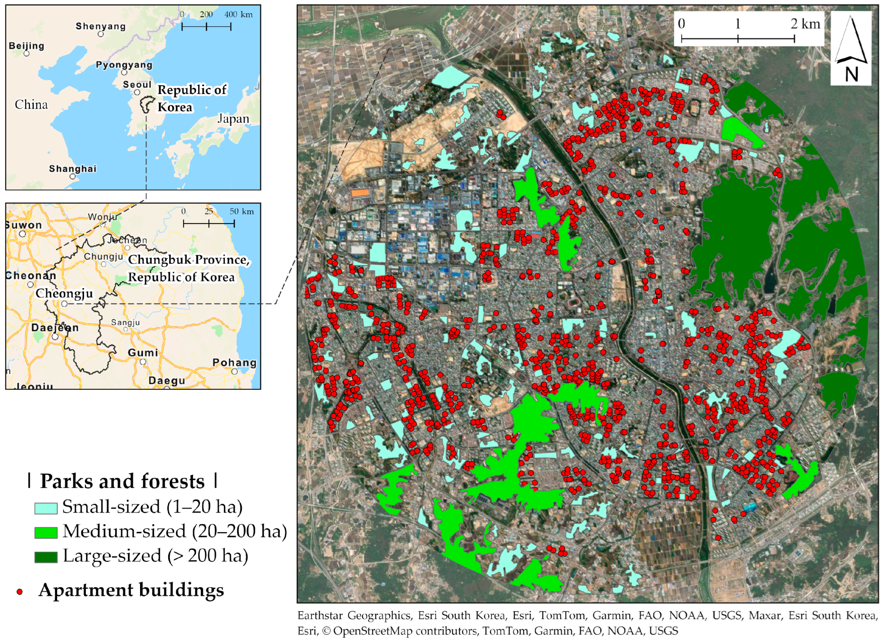
2.2. Study Area and Data
3. Empirical Analysis, Results, and Discussion
3.1. SAR Model
3.2. GAM
4. Conclusions
Author Contributions
Funding
Data Availability Statement
Acknowledgments
Conflicts of Interest
References
- Swanwick, C.; Dunnett, N.; Woolley, H. Nature, role and value of green space in towns and cities: An overview. Built Environ. 2003, 29, 94–106. [Google Scholar] [CrossRef]
- Kawachi, I.; Berkman, L.F. Social ties and mental health. J. Urban Health 2001, 78, 458–467. [Google Scholar] [CrossRef] [PubMed]
- Loukaitou-Sideris, A.; Levy-Storms, L.; Chen, L.; Brozen, M. Parks for an aging population: Needs and preferences of low-income seniors in Los Angeles. J. Am. Plan. Assoc. 2016, 82, 236–251. [Google Scholar] [CrossRef]
- Enssle, F.; Kabisch, N. Urban green spaces for the social interaction, health and well-being of older people—An integrated view of urban ecosystem services and socio-environmental justice. Environ. Sci. Policy 2020, 109, 36–44. [Google Scholar] [CrossRef]
- Bolund, P.; Hunhammar, S. Ecosystem services in urban areas. Ecol. Econ. 1999, 29, 293–301. [Google Scholar] [CrossRef]
- Nowak, D.J.; Hirabayashi, S.; Bodine, A.; Greenfield, E. Tree and forest effects on air quality and human health in the United States. Environ. Pollut. 2014, 193, 119–129. [Google Scholar] [CrossRef] [PubMed]
- Baycan-Levent, T.; Nijkamp, P. Evaluation of urban green spaces. In Beyond Benefit Cost Analysis: Accounting for Non-Market Values in Planning Evaluation; Miller, D., Patassini, D., Eds.; Ashgate Publishing: Aldershot, UK, 2005; pp. 63–87. [Google Scholar]
- Arvanitidis, P.A.; Lalenis, K.; Petrakos, G.; Psycharis, Y. Economic aspects of urban green space: A survey of perceptions and attitudes. Int. J. Environ. Technol. Manag. 2009, 11, 143–168. [Google Scholar] [CrossRef]
- Crompton, J.L. The impact of parks on property values: Empirical evidence from the past two decades in the United States. Manag. Leis. 2005, 10, 203–218. [Google Scholar] [CrossRef]
- Alonso, W. Location and Land Use; Harvard University Press: Cambridge, MA, USA, 1964. [Google Scholar]
- Brueckner, J.K.; Thisse, J.F.; Zenou, Y. Why is central Paris rich and downtown Detroit poor?: An amenity-based theory. Eur. Econ. Rev. 1999, 43, 91–107. [Google Scholar] [CrossRef]
- Cho, C.J. Amenities and urban residential structure: An amenity-embedded model of residential choice. Pap. Reg. Sci. 2001, 80, 483–498. [Google Scholar]
- O’Sullivan, A. Urban Economics; Irwin Professional Publishing: Chicago, IL, USA, 1996. [Google Scholar]
- Votsis, A. Planning for green infrastructure: The spatial effects of parks, forests, and fields on Helsinki’s apartment prices. Ecol. Econ. 2017, 132, 279–289. [Google Scholar] [CrossRef]
- Papastergiou, E.; Latinopoulos, D.; Evdou, M.; Kalogeresis, A. Exploring associations between subjective well-being and non-market values when used in the evaluation of urban green spaces: A scoping review. Land 2023, 12, 700. [Google Scholar] [CrossRef]
- Baycan-Levent, T.; Vreeker, R.; Nijkamp, P. A multi-criteria evaluation of green spaces in European cities. Eur. Urban. Reg. Stud. 2009, 16, 193–213. [Google Scholar] [CrossRef]
- More, T.A.; Stevens, T.; Allen, P.G. Valuation of urban parks. Landsc. Urban Plan. 1988, 15, 139–152. [Google Scholar] [CrossRef]
- Pearce, D. Economics and Environment: Essays on Ecological Economics and Sustainable Development; Edward Elgar Publishing: Cheltenham Glos, UK, 1999. [Google Scholar]
- LeSage, J.; Pace, R.K. Introduction to Spatial Econometrics; Chapman and Hall/CRC: New York, NY, USA, 2009. [Google Scholar]
- Gleditsch, K.; Ward, M.D. Spatial Regression Models; Sage Publications Inc.: Thousand Oaks, CA, USA, 2008; Volume 155. [Google Scholar]
- Lin, T.M.; Wu, E.E.; Lee, F.Y. Neighborhood influence on the formation of national identity in Taiwan: Spatial regression with disjoint neighborhoods. Political Res. Q. 2006, 59, 35–46. [Google Scholar] [CrossRef]
- Elhorst, J.P. Applied spatial econometrics: Raising the bar. Spat. Econ. Anal. 2010, 5, 9–28. [Google Scholar] [CrossRef]
- Fischer, M.M.; Wang, J. Spatial Data Analysis: Models, Methods, and Techniques; Springer: London, UK, 2011. [Google Scholar]
- Golgher, A.B.; Voss, P.R. How to interpret the coefficients of spatial models: Spillovers, direct and indirect effects. Spat. Demogr. 2016, 4, 175–205. [Google Scholar] [CrossRef]
- LeSage, J.P. What regional scientists need to know about spatial econometrics. Rev. Reg. Stud. 2014, 44, 13–32. [Google Scholar]
- Seya, H.; Yoshida, T.; Yamagata, Y. Spatial econometric models. In Spatial Analysis Using Big Data; Yamagata, Y., Seya, H., Eds.; Academic Press: London, UK, 2020; pp. 113–158. [Google Scholar]
- Wood, S.N. Generalized Additive Models: An Introduction with R; Chapman and Hall/CRC Press: Boca Raton, FL, USA, 2017. [Google Scholar]
- Wood, S.N.; Pya, N.; Säfken, B. Smoothing parameter and model selection for general smooth models. J. Am. Stat. Assoc. 2016, 111, 1548–1563. [Google Scholar] [CrossRef]
- Baayen, R.H.; Linke, M. An introduction to the generalized additive model. In A Practical Handbook of Corpus Linguistics; Paquot, M., Gries, S.T., Eds.; Springer: New York, NY, USA, 2020; pp. 563–591. [Google Scholar]
- Simpson, G.L. Modelling palaeoecological time series using generalized additive models. Front. Ecol. Evol. 2018, 6, 149–170. [Google Scholar] [CrossRef]
- Larsen, K. GAM: The predictive modeling silver bullet. Multithreaded. Stitch Fix 2015, 30, 1–27. [Google Scholar]
- Laurinec, P. Doing Magic and Analyzing Seasonal Time Series with GAM (Generalized Additive Model) in R. Available online: https://petolau.github.io/Analyzing-double-seasonal-time-series-with-GAM-in-R/ (accessed on 3 March 2024).
- Wood, S.N. Fast stable restricted maximum likelihood and marginal likelihood estimation of semiparametric generalized linear models. J. R. Stat. Soc. B 2011, 73, 3–36. [Google Scholar] [CrossRef]
- Reiss, P.T.; Todd Ogden, R. Smoothing parameter selection for a class of semiparametric linear models. J. R. Stat. Soc. Ser. B Stat. Methodol. 2009, 71, 505–523. [Google Scholar] [CrossRef]
- Chungbuk. Statistical Information System. Available online: https://www.chungbuk.go.kr/stat/index.do (accessed on 3 March 2024).
- Cheongju City. Statistical Information System. Available online: https://www.cheongju.go.kr/stat/index.do (accessed on 3 March 2024).
- Haeler, E.; Bolte, A.; Buchacher, R.; Hänninen, H.; Jandl, R.; Juutinen, A.; Kuhlmey, K.; Kurttila, M.; Lidestav, G.; Mäkipää, R.; et al. Forest subsidy distribution in five European countries. For. Policy Econ. 2023, 146, 102882. [Google Scholar] [CrossRef]
- ESRI. ArcGIS Pro; Version 3.1; Esri Inc.: Redlands, CA, USA, 2023. [Google Scholar]
- Bivand, R. Comparing estimation methods for spatial econometrics techniques using R. In NHH Dept. of Economics Discussion Paper No. 26; Elsevier: Amsterdam, The Netherlands, 2010. [Google Scholar]
- Bivand, R.; Millo, G.; Piras, G. A review of software for spatial econometrics in R. Mathematics 2021, 9, 1276. [Google Scholar] [CrossRef]
- Kelejian, H.H.; Prucha, I.R. HAC estimation in a spatial framework. J. Econom. 2007, 140, 131–154. [Google Scholar] [CrossRef]
- Kelejian, H.H.; Prucha, I.R. The relative efficiencies of various predictors in spatial econometric models containing spatial lags. Reg. Sci. Urban Econ. 2007, 37, 363–374. [Google Scholar] [CrossRef]
- Piras, G. sphet: Spatial models with heteroskedastic innovations in R. J. Stat. Softw. 2010, 35, 1–21. [Google Scholar] [CrossRef]
- Bivand, R.; Anselin, L.; Berke, O.; Bernat, A.; Carvalho, M.; Chun, Y.; Dormann, C.; Dray, S.; Halbersma, R.; Lewin-Koh, N. Spdep: Spatial Dependence: Weighting Schemes, Statistics and Models. R Package Version 0.5-31, URL. 2011. Available online: http://CRAN.R-project.org/package=spdep (accessed on 3 March 2024).
- Ozus, E.; Dokmeci, V.; Kiroglu, G.; Egdemir, G. Spatial analysis of residential prices in Istanbul. Eur. Plan. Stud. 2007, 15, 707–721. [Google Scholar] [CrossRef]
- Ligus, M.; Peternek, P. Measuring structural, location and environmental effects: A hedonic analysis of housing market in Wroclaw, Poland. Procedia Soc. Behav. Sci. 2016, 220, 251–260. [Google Scholar] [CrossRef]
- Tyrväinen, L.; Miettinen, A. Property prices and urban forest amenities. J. Environ. Econ. Manag. 2000, 39, 205–223. [Google Scholar] [CrossRef]
- Melichar, J.; Vojáček, O.; Rieger, P.; Jedlička, K. Measuring the value of urban forest using the hedonic price approach. Czech Reg. Stud. 2009, 2, 13–20. [Google Scholar]
- Landis, J.; Reina, V.J. Do restrictive land use regulations make housing more expensive everywhere? Econ. Dev. Q. 2021, 35, 305–324. [Google Scholar] [CrossRef]
- Ewane, E.B.; Bajaj, S.; Velasquez-Camacho, L.; Srinivasan, S.; Maeng, J.; Singla, A.; Luber, A.; de-Miguel, S.; Richardson, G.; Broadbent, E.N.; et al. Influence of urban forests on residential property values: A systematic review of remote sensing-based studies. Heliyon 2023, 9, e20408. [Google Scholar] [CrossRef]
- Łaszkiewicz, E.; Heyman, A.; Chen, X.; Cimburova, Z.; Nowell, M.; Barton, D.N. Valuing access to urban greenspace using non-linear distance decay in hedonic property pricing. Ecosyst. Serv. 2022, 53, 101394. [Google Scholar] [CrossRef]
- Marra, G.; Wood, S.N. Coverage properties of confidence intervals for generalized additive model components. Scand. J. Stat. 2012, 39, 53–74. [Google Scholar] [CrossRef]
- Paquot, M.; Gries, S.T. A Practical Handbook of Corpus Linguistics; Springer Nature: Berlin/Heidelberg, Germany, 2021; p. 686. [Google Scholar]
- Crompton, J.L. The impact of parks on property values: A review of the empirical evidence. J. Leis. Res. 2001, 33, 1–31. [Google Scholar] [CrossRef]
- Zhou, H.; Wang, J.; Wilson, K. Impacts of perceived safety and beauty of park environments on time spent in parks: Examining the potential of street view imagery and phone-based GPS data. Int. J. Appl. Earth Obs. Geoinf. 2022, 115, 103078. [Google Scholar] [CrossRef]


| Variable | Description | Unit | Mean | Std. Dev. |
|---|---|---|---|---|
| Dependent variable | ||||
| PRICE | Apartment selling price per m2 (in 2018 price) | USD 7.69/m2 (KRW 10,000/m2) | 217.19 | 77.41 |
| Structural variables | ||||
| FLOORAREA | Total floor area | m2 | 76.10 | 31.22 |
| FLOOR | The floor on which the unit is situated | 7.19 | 4.08 | |
| AGE | Building age (the period between the year the building was constructed and the year the property was sold) | Years | 21.40 | 9.97 |
| Locational variables | ||||
| DISBUSTOP | Road distance to nearest bus stop | m | 244.89 | 121.97 |
| DISPROVIN | Road distance to provincial government office | m | 3799.00 | 1560.84 |
| DISKINDER | Road distance to nearest kindergarten | m | 557.05 | 333.26 |
| DISELEMENT | Road distance to nearest elementary school | m | 607.20 | 289.65 |
| DISHIGH | Road distance to nearest high school | m | 921.32 | 408.27 |
| DISHOSPIT | Road distance to nearest general hospital | m | 1570.79 | 626.86 |
| DISHOPING | Road distance to nearest shopping center | m | 1666.16 | 767.20 |
| Environmental variables | ||||
| DISROAD | Euclidean distance to adjacent street | m | 82.37 | 55.26 |
| DISGREENSM | Road distance to nearest small-sized green space | m | 451.75 | 300.15 |
| DISGREENMD | Road distance to nearest medium-sized green space | m | 1481.42 | 946.42 |
| DISGREENLR | Road distance to nearest large-sized green space | m | 3331.16 | 1908.18 |
| Variable | Coeff. | Std. Error | t-Value | p-Value | |
|---|---|---|---|---|---|
| Wy | 0.086802 | 0.046722 | 1.8578 | 0.063192 | • |
| (Intercept) | 5.148492 | 0.255860 | 20.1223 | 0.000000 | *** |
| FLOORAREA | −0.000596 | 0.000197 | −3.0294 | 0.002450 | ** |
| FLOOR | 0.017397 | 0.001762 | 9.8760 | 0.000000 | *** |
| AGE | −0.021964 | 0.001069 | −20.5490 | 0.000000 | *** |
| DISBUSTOP | −0.000132 | 0.000047 | −2.8397 | 0.004515 | ** |
| DISPROVIN | 0.000037 | 0.000007 | 5.1946 | 0.000000 | *** |
| DISKINDER | 0.000011 | 0.000025 | 0.4303 | 0.666945 | |
| DISELEMENT | −0.000026 | 0.000028 | −0.9358 | 0.349394 | |
| DISHIGH | −0.000090 | 0.000016 | −5.6653 | 0.000000 | *** |
| DISHOSPIT | 0.000022 | 0.000010 | 2.0999 | 0.035739 | * |
| DISHOPING | 0.000045 | 0.000009 | 4.9963 | 0.000000 | *** |
| DISROAD | −0.000271 | 0.000108 | 2.5158 | 0.011876 | * |
| DISGREENSM | −0.000034 | 0.000020 | −1.6777 | 0.093397 | • |
| DISGREENMD | −0.000014 | 0.000006 | −2.4892 | 0.012802 | * |
| DISGREENLR | 0.000009 | 0.000005 | 1.9282 | 0.053825 | • |
| Residuals: | |||||
| Minimum | 1st quartile | Median | 3rd quartile | Maximum | |
| −0.970288 | −0.086318 | 0.017733 | 0.104464 | 0.614417 | |
| Variable | Direct | Indirect | Total |
|---|---|---|---|
| FLOORAREA | −0.000596 | −0.000056 | −0.000653 |
| FLOOR | 0.017415 | 0.001635 | 0.019051 |
| AGE | −0.021987 | −0.002064 | −0.024052 |
| DISBUSTOP | −0.000133 | −0.000012 | −0.000145 |
| DISPROVIN | 0.000037 | 0.000003 | 0.000041 |
| DISKINDER | 0.000011 | 0.000001 | 0.000012 |
| DISELEMENT | −0.000026 | −0.000002 | −0.000028 |
| DISHIGH | −0.000090 | −0.000008 | −0.000098 |
| DISHOSPIT | 0.000022 | 0.000002 | 0.000024 |
| DISHOPING | 0.000045 | 0.000004 | 0.000049 |
| DISROAD | −0.000271 | −0.000025 | −0.000297 |
| DISGREENSM | −0.000034 | −0.000003 | −0.000037 |
| DISGREENMD | −0.000014 | −0.000001 | −0.000015 |
| DISGREENLR | 0.000009 | 0.000001 | 0.000010 |
| A. Parametric coefficients | |||||
| Variable | Coeff. | Std. error | t-value | p-value | |
| (Intercept) | 5.727103 | 0.031545 | 181.555 | 0.000000 | *** |
| FLOORAREA | −0.000673 | 0.000189 | −3.544 | 0.000414 | *** |
| FLOOR | 0.018206 | 0.001997 | 9.115 | 0.000000 | *** |
| AGE | −0.022872 | 0.000825 | −27.725 | 0.000000 | *** |
| B. Approximate significance of smooth terms | |||||
| Smooth term | EDF (1) | Ref. DF (2) | F-value | p-value | |
| s(DISBUSTOP) | 7.401 | 8.371 | 1.525 | 0.142935 | |
| s(DISPROVIN) | 45.195 | 47.862 | 2.524 | 0.000000 | *** |
| s(DISKINDER) | 7.093 | 7.999 | 5.113 | 0.000002 | *** |
| s(DISELEMENT) | 6.592 | 7.596 | 2.448 | 0.012865 | * |
| s(DISHIGH) | 8.421 | 8.858 | 4.458 | 0.000009 | *** |
| s(DISHOSPIT) | 1.385 | 1.675 | 2.223 | 0.137499 | |
| s(DISHOPING) | 14.980 | 17.175 | 2.415 | 0.000000 | *** |
| s(DISROAD) | 4.511 | 5.578 | 2.757 | 0.014079 | * |
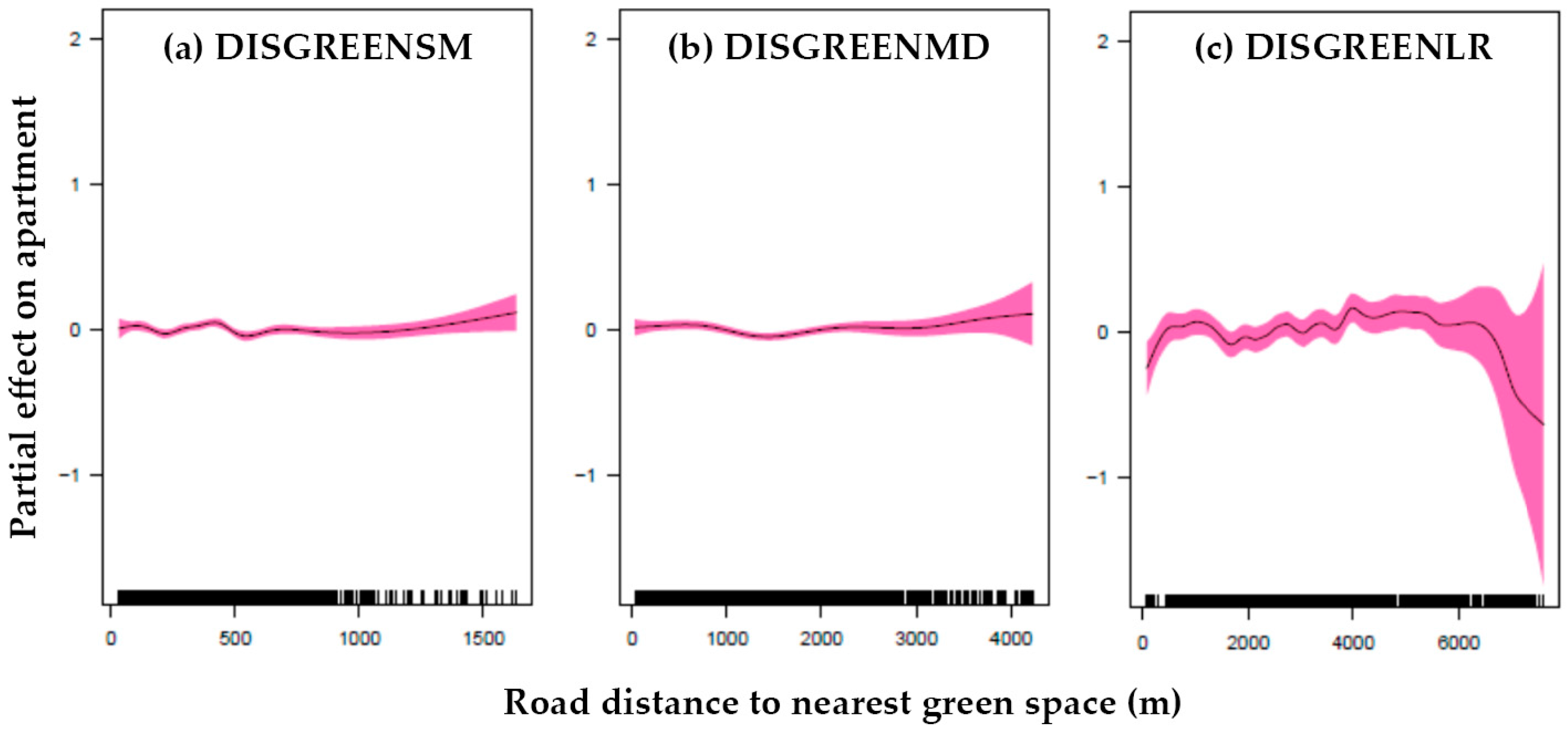
| s(DISGREENSM) | 8.891 | 8.891 | 2.701 | 0.003640 | ** |
| s(DISGREENMD) | 6.340 | 7.479 | 2.724 | 0.007506 | ** |
| s(DISGREENLR) | 25.348 | 30.745 | 2.113 | 0.000368 | *** |
| R-sq.(adj) = 0.813 Deviance explained = 83.7% GCV = 0.025496 Scale est. = 0.024245 n = 1102 | |||||
Disclaimer/Publisher’s Note: The statements, opinions and data contained in all publications are solely those of the individual author(s) and contributor(s) and not of MDPI and/or the editor(s). MDPI and/or the editor(s) disclaim responsibility for any injury to people or property resulting from any ideas, methods, instructions or products referred to in the content. |
© 2024 by the authors. Licensee MDPI, Basel, Switzerland. This article is an open access article distributed under the terms and conditions of the Creative Commons Attribution (CC BY) license (https://creativecommons.org/licenses/by/4.0/).
Share and Cite
Cho, C.-J.; Cheon, K.; Kang, W. Assessment of the Spatial Variation of the Economic Benefits of Urban Green Spaces in a Highly Urbanized Area. Land 2024, 13, 577. https://doi.org/10.3390/land13050577
Cho C-J, Cheon K, Kang W. Assessment of the Spatial Variation of the Economic Benefits of Urban Green Spaces in a Highly Urbanized Area. Land. 2024; 13(5):577. https://doi.org/10.3390/land13050577
Chicago/Turabian StyleCho, Cheol-Joo, Kwangil Cheon, and Wanmo Kang. 2024. "Assessment of the Spatial Variation of the Economic Benefits of Urban Green Spaces in a Highly Urbanized Area" Land 13, no. 5: 577. https://doi.org/10.3390/land13050577
APA StyleCho, C.-J., Cheon, K., & Kang, W. (2024). Assessment of the Spatial Variation of the Economic Benefits of Urban Green Spaces in a Highly Urbanized Area. Land, 13(5), 577. https://doi.org/10.3390/land13050577