
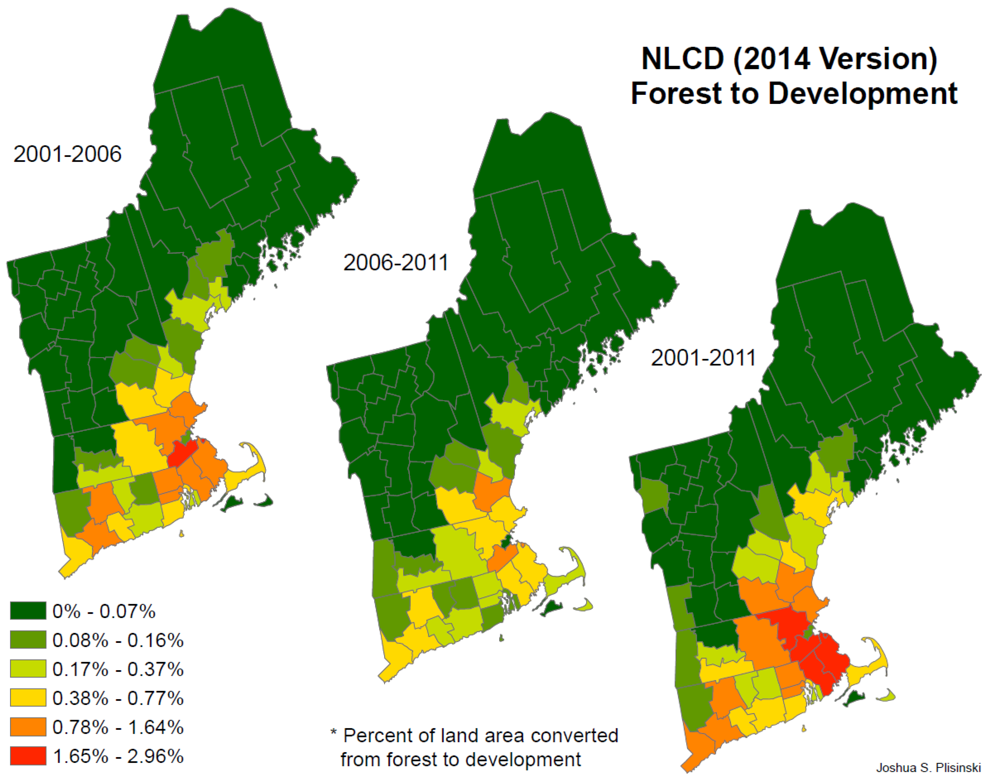
Patterns and Predictors of Recent Forest Conversion in New England

Abstract
:1. Introduction
2. Materials and Methods
2.1. Study Area
2.2. Data
2.3. Analysis
3. Results
4. Discussion
Supplementary Materials
Acknowledgments
Author Contributions
Conflicts of Interest
Abbreviations
| BRT | boosted regression tree |
| NLCD | National Land Cover Database |
Appendix A

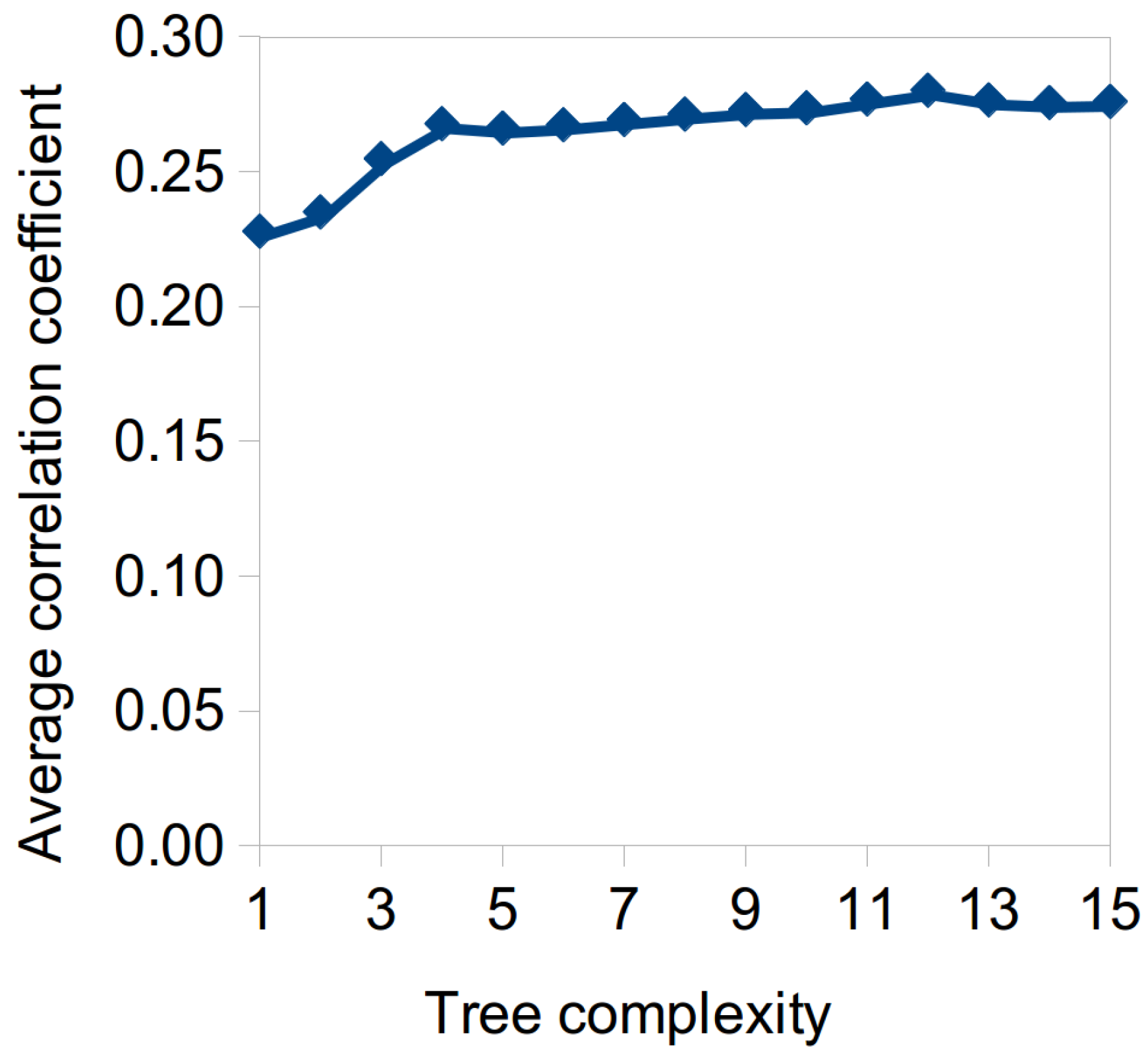
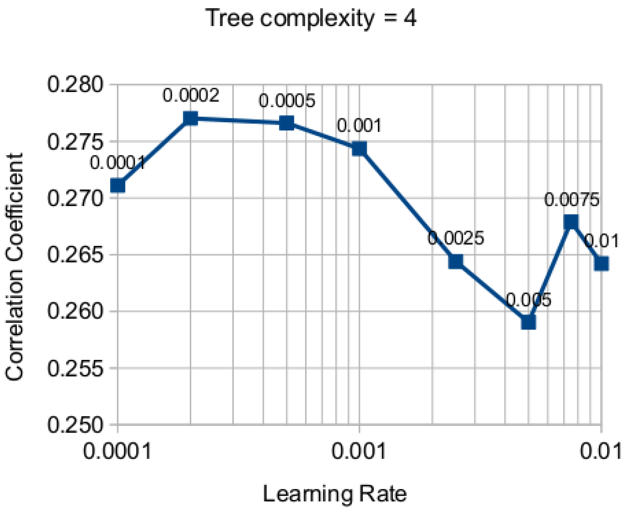
| Tree Complexity | Learning Rate | ||||||
|---|---|---|---|---|---|---|---|
| 0.0100 | 0.0075 | 0.0050 | 0.0025 | 0.0010 | 0.0005 | Row Mean | |
| 1 | 0.2150 | 0.2171 | 0.2212 | 0.2329 | 0.2396 | 0.2416 | 0.2279 |
| 2 | 0.2167 | 0.2273 | 0.2291 | 0.2353 | 0.2488 | 0.2529 | 0.2350 |
| 3 | 0.2447 | 0.2539 | 0.2522 | 0.2556 | 0.2615 | 0.2609 | 0.2548 |
| 4 | 0.2642 | 0.2679 | 0.2590 | 0.2644 | 0.2744 | 0.2766 | 0.2678 |
| 5 | 0.2585 | 0.2461 | 0.2648 | 0.2706 | 0.2762 | 0.2805 | 0.2661 |
| 6 | 0.2514 | 0.2610 | 0.2679 | 0.2699 | 0.2744 | 0.2794 | 0.2673 |
| 7 | 0.2688 | 0.2602 | 0.2658 | 0.2680 | 0.2688 | 0.2843 | 0.2693 |
| 8 | 0.2620 | 0.2654 | 0.2570 | 0.2753 | 0.2822 | 0.2860 | 0.2713 |
| 9 | 0.2723 | 0.2673 | 0.2684 | 0.2679 | 0.2782 | 0.2842 | 0.2730 |
| 10 | 0.2657 | 0.2536 | 0.2700 | 0.2752 | 0.2876 | 0.2899 | 0.2736 |
| 11 | 0.2569 | 0.2749 | 0.2787 | 0.2757 | 0.2856 | 0.2899 | 0.2770 |
| 12 | 0.2766 | 0.2892 | 0.2640 | 0.2752 | 0.2840 | 0.2920 | 0.2802 |
| 13 | 0.2659 | 0.2658 | 0.2821 | 0.2756 | 0.2847 | 0.2854 | 0.2766 |
| 14 | 0.2662 | 0.2777 | 0.2682 | 0.2719 | 0.2840 | 0.2857 | 0.2756 |
| 15 | 0.2735 | 0.2732 | 0.2664 | 0.2721 | 0.2827 | 0.2882 | 0.2760 |


References
- Breunig, K. Losing Ground: At What Cost? Changes in Land Use and Their Impacts on Habitat, Biodiversity and Ecosystem Services in Massachusetts; Summary Report; Advocacy Department, Mass Audubon: Lincoln, MA, USA, 2003. [Google Scholar]
- Foster, D.; Donahue, B.M.; Kittredge, D.B.; Lambert, K.F.; Hunter, M.L.; Hall, B.R.; Irland, L.C.; Lilieholm, R.J.; Orwig, D.A.; D’Amato, A.W.; et al. Wildlands and Woodlands: A Vision for the New England Landscape; Harvard Forest; Harvard University Press: Cambridge, MA, USA, 2010. [Google Scholar]
- Levesque, C.A. New Hampshire Statewide Forest Resources Assessment—2010: Important Data and Information about New Hampshire’s Forests; New Hampshire Department of Resources and Economic Development Division of Forests and Lands: Concord, NH, USA, 2010. [Google Scholar]
- Zheng, D.; Heath, L.S.; Ducey, M.J.; Butler, B. Relationships between major ownerships, forest aboveground biomass distributions, and landscape dynamics in the New England Region of USA. Environ. Manag. 2010, 45, 377–386. [Google Scholar] [CrossRef] [PubMed]
- Zheng, D.; Heath, L.S.; Ducey, M.J. Potential overestimation of carbon sequestration in the forested wildland-urban interface in Northern New England. J. For. 2012, 110, 105–111. [Google Scholar] [CrossRef]
- Zheng, D.; Ducey, M.J.; Heath, L.S. Assessing net carbon sequestration on urban and community forests of northern New England, USA. Urban For. Urban Green. 2013, 12, 61–68. [Google Scholar] [CrossRef]
- Blumstein, M.; Thompson, J.R. Land-use impacts on the quantity and configuration of ecosystem service provisioning in Massachusetts, USA. J. Appl. Ecol. 2015, 52, 1009–1019. [Google Scholar] [CrossRef]
- USDA Forest Service. Standard Tables of Forest Carbon Stock Estimates by State; USDA Forest Service: Washington, DC, USA, 2014. [Google Scholar]
- Smith, J.E.; Heath, L.S.; Nichols, M.C. US Forest Carbon Calculation Tool: Forest-Land Carbon Stocks and Net Annual Stock Change; General Technical Report NRS-13; USDA Forest Service, Northern Research Station: Durham, NH, USA, 2007. [Google Scholar]
- U.S. Environmental Protection Agency. Land Use, Land-Use Change, and Forestry. In Inventory of U.S. Greenhouse Gas Emissions and Sinks: 1990–2013; Number EPA 430-R- 15 -004; U.S. Environmental Protection Agency: Washington, DC, USA, 2015. [Google Scholar]
- Meyer, S.R.; Johnson, M.L.; Lilieholm, R.J.; Cronan, C.S. Development of a stakeholder-driven spatial modeling framework for strategic landscape planning using Bayesian networks across two urban-rural gradients in Maine, USA. Ecol. Model. 2014, 291, 42–57. [Google Scholar] [CrossRef]
- Bierwagen, B.G.; Theobald, D.M.; Pyke, C.R.; Choate, A.; Groth, P.; Thomas, J.V.; Morefield, P. National housing and impervious surface scenarios for integrated climate impact assessments. Proc. Natl. Acad. Sci. USA 2010, 107, 20887–20892. [Google Scholar] [CrossRef] [PubMed]
- Stein, S.M.; McRoberts, R.E.; Mahal, L.G.; Carr, M.A.; Alig, R.J.; Comas, S.J.; Theobald, D.M.; Cundiff, A. Private Forests, Public Benefits: Increased Housing Density and Other Pressures on Private Forests Contributions; General Technical Report PNW-GTR-795; U.S. Department of Agriculture, Forest Service, Pacific Northwest Research Station: Portland, OR, USA, 2009.
- Thompson, J.; Fallon Lambert, K.; Foster, D.; Blumstein, M.; Broadbent, E.; Almeyda Zambrano, A. Changes to the Land: Four Scenarios for the Future of the Massachusetts Landscape; Technical Report; Harvard Forest: Petersham, MA, USA, 2014. [Google Scholar]
- Drummond, M.A.; Loveland, T.R. Land-use pressure and a transition to forest-cover loss in the Eastern United States. BioScience 2010, 60, 286–298. [Google Scholar] [CrossRef]
- Jeon, S.B.; Olofsson, P.; Woodcock, C.E. Land use change in New England: A reversal of the forest transition. J. Land Use Sci. 2014, 9, 105–130. [Google Scholar] [CrossRef]
- Alcamo, J.; Kok, K.; Busch, G.; Priess, J.A.; Eickhout, B.; Rounsevell, M.; Rothman, D.S.; Heistermann, M. Searching for the future of land: Scenarios from the local to global scale. In Land-Use and Land-Cover Change; Springer: Berlin, Germany, 2006; pp. 137–155. [Google Scholar]
- Tayyebi, A.; Pijanowski, B.C.; Linderman, M.; Gratton, C. Comparing three global parametric and local non-parametric models to simulate land use change in diverse areas of the world. Environ. Model. Softw. 2014, 59, 202–221. [Google Scholar] [CrossRef]
- Thompson, J.R.; Foster, D.R.; Scheller, R.; Kittredge, D. The influence of land use and climate change on forest biomass and composition in Massachusetts, USA. Ecol. Appl. 2011, 21, 2425–2444. [Google Scholar] [CrossRef] [PubMed]
- Rounsevell, M.; Reginster, I.; Araújo, M.; Carter, T.; Dendoncker, N.; Ewert, F.; House, J.; Kankaanpää, S.; Leemans, R.; Metzger, M.; et al. A coherent set of future land use change scenarios for Europe. Agric. Ecosyst. Environ. 2006, 114, 57–68. [Google Scholar] [CrossRef]
- Schneider, L.C.; Pontius, R.G. Modeling land-use change in the Ipswich watershed, Massachusetts, USA. Agric. Ecosyst. Environ. 2001, 85, 83–94. [Google Scholar] [CrossRef]
- Sohl, T.; Sayler, K. Using the FORE-SCE model to project land-cover change in the southeastern United States. Ecol. Model. 2008, 219, 49–65. [Google Scholar] [CrossRef]
- Radeloff, V.C.; Nelson, E.; Plantinga, A.J.; Lewis, D.J.; Helmers, D.; Lawler, J.J.; Withey, J.C.; Beaudry, F.; Martinuzzi, S.; Butsic, V.; et al. Economic-based projections of future land-use under alternative economic policy scenarios in the conterminous US. Ecol. Appl. 2012, 22, 1036–1049. [Google Scholar] [CrossRef] [PubMed]
- Mockrin, M.H.; Stewart, S.I.; Radeloff, V.C.; Hammer, R.B.; Johnson, K.M. Spatial and temporal residential density patterns from 1940 to 2000 in and around the Northern Forest of the Northeastern United States. Popul. Environ. 2012, 34, 400–419. [Google Scholar] [CrossRef]
- Johnson, K.M.; Beale, C.L. Nonmetro recreation counties: Their identification and rapid growth. Rural Am. 2002, 17, 4. [Google Scholar]
- Tyrrell, M.; Hall, M.; Sampson, R. Dynamic Models of Land Use Change in Northeastern USA: Deveoping Tools Techniques, and Talents for Effective Conservation Action; Yale University School of Forestry and Environmental Studies: New Haven, CT, USA, 2004. [Google Scholar]
- Duveneck, M.J.; Thompson, J.R.; Wilson, B.T. An imputed forest composition map for New England screened by species range boundaries. For. Ecol. Manag. 2015, 347, 107–115. [Google Scholar] [CrossRef]
- Foster, D.R.; Aber, J.D. (Eds.) Forests in Time: The Environmental Consequences of 1000 Years of Change in New England; Yale University Press: New Haven, CT, USA, 2004.
- Homer, C.G.; Dewitz, J.A.; Yang, L.; Jin, S.; Danielson, P.; Xian, G.; Coulston, J.; Herold, N.D.; Wickham, J.D.; Megown, K. Completion of the 2011 National Land Cover Database for the conterminous United States - Representing a decade of land cover change information. Photogramm. Eng. Remote Sens. 2015, 81, 345–354. [Google Scholar]
- Gesch, D.; Oimoen, M.; Greenlee, S.; Nelson, C.; Steuck, M.; Tyler, D. The National Elevation Dataset. Photogramm. Eng. Remote Sens. 2002, 68, 5–11. [Google Scholar]
- QGIS Development Team. QGIS Geographic Information System; Open Source Geospatial Foundation Project; Open Source Geospatial Foundation: Beaverton, OR, USA, 2015. [Google Scholar]
- R Core Team. R: A Language and Environment for Statistical Computing; R Foundation for Statistical Computing: Vienna, Austria, 2015. [Google Scholar]
- Dormann, C.F.; Elith, J.; Bacher, S.; Buchmann, C.; Carl, G.; Carré, G.; Marquéz, J.R.G.; Gruber, B.; Lafourcade, B.; Leitão, P.J.; et al. Collinearity: A review of methods to deal with it and a simulation study evaluating their performance. Ecography 2013, 36, 27–46. [Google Scholar] [CrossRef]
- Levers, C.; Verkerk, P.J.; Müller, D.; Verburg, P.H.; Butsic, V.; Leitão, P.J.; Lindner, M.; Kuemmerle, T. Drivers of forest harvesting intensity patterns in Europe. For. Ecol. Manag. 2014, 315, 160–172. [Google Scholar] [CrossRef]
- Elith, J.; Leathwick, J.R.; Hastie, T. A working guide to boosted regression trees. J. Anim. Ecol. 2008, 77, 802–813. [Google Scholar] [CrossRef] [PubMed]
- Elith, J.; Graham, C.H.; Anderson, R.P.; Dudík, M.; Ferrier, S.; Guisan, A.; Hijmans, R.J.; Huettmann, F.; Leathwick, J.R.; Lehmann, A.; et al. Novel methods improve prediction of species’ distributions from occurrence data. Ecography 2006, 29, 129–151. [Google Scholar] [CrossRef]
- Leathwick, J.R.; Elith, J.; Francis, M.P.; Hastie, T.; Taylor, P. Variation in demersal fish species richness in the oceans surrounding New Zealand: An analysis using boosted regression trees. Mar. Ecol. Prog. Ser. 2006, 321, 267–281. [Google Scholar] [CrossRef]
- Marmion, M.; Luoto, M.; Heikkinen, R.K.; Thuiller, W. The performance of state-of-the-art modelling techniques depends on geographical distribution of species. Ecol. Model. 2009, 220, 3512–3520. [Google Scholar] [CrossRef]
- Thomaes, A.; Kervyn, T.; Maes, D. Applying species distribution modelling for the conservation of the threatened saproxylic Stag Beetle (Lucanus cervus). Biol. Conserv. 2008, 141, 1400–1410. [Google Scholar] [CrossRef]
- Li, X.; Wang, Y. Applying various algorithms for species distribution modelling. Integr. Zool. 2013, 8, 124–135. [Google Scholar] [CrossRef] [PubMed]
- Johnstone, J.F.; Hollingsworth, T.N.; Chapin, F.S.; Mack, M.C. Changes in fire regime break the legacy lock on successional trajectories in Alaskan boreal forest. Glob. Chang. Biol. 2010, 16, 1281–1295. [Google Scholar] [CrossRef]
- Greve, M.; Lykke, A.M.; Blach-Overgaard, A.; Svenning, J.C. Environmental and anthropogenic determinants of vegetation distribution across Africa: Determinants of African vegetation distribution. Glob. Ecol. Biogeogr. 2011, 20, 661–674. [Google Scholar] [CrossRef]
- Snelder, T.H.; Lamouroux, N.; Leathwick, J.R.; Pella, H.; Sauquet, E.; Shankar, U. Predictive mapping of the natural flow regimes of France. J. Hydrol. 2009, 373, 57–67. [Google Scholar] [CrossRef]
- Nolan, B.T.; Fienen, M.N.; Lorenz, D.L. A statistical learning framework for groundwater nitrate models of the Central Valley, California, USA. J. Hydrol. 2015, 531, 902–911. [Google Scholar] [CrossRef]
- Marmion, M.; Hjort, J.; Thuiller, W.; Luoto, M. A comparison of predictive methods in modelling the distribution of periglacial landforms in Finnish Lapland. Earth Surf. Process. Landf. 2008, 33, 2241–2254. [Google Scholar] [CrossRef]
- Martin, M.P.; Wattenbach, M.; Smith, P.; Meersmans, J.; Jolivet, C.; Boulonne, L.; Arrouays, D. Spatial distribution of soil organic carbon stocks in France. Biogeosciences 2011, 8, 1053–1065. [Google Scholar] [CrossRef]
- Mosleh, Z.; Salehi, M.H.; Jafari, A.; Borujeni, I.E.; Mehnatkesh, A. The effectiveness of digital soil mapping to predict soil properties over low-relief areas. Environ. Monit. Assess. 2016, 188, 195. [Google Scholar] [CrossRef] [PubMed]
- Parisien, M.A.; Moritz, M.A. Environmental controls on the distribution of wildfire at multiple spatial scales. Ecol. Monogr. 2009, 79, 127–154. [Google Scholar] [CrossRef]
- Müller, D.; Leitão, P.J.; Sikor, T. Comparing the determinants of cropland abandonment in Albania and Romania using boosted regression trees. Agric. Syst. 2013, 117, 66–77. [Google Scholar] [CrossRef]
- Linard, C.; Tatem, A.J.; Gilbert, M. Modelling spatial patterns of urban growth in Africa. Appl. Geogr. 2013, 44, 23–32. [Google Scholar] [CrossRef] [PubMed]
- Aertsen, W.; Kint, V.; van Orshoven, J.; Özkan, K.; Muys, B. Comparison and ranking of different modelling techniques for prediction of site index in Mediterranean mountain forests. Ecol. Model. 2010, 221, 1119–1130. [Google Scholar] [CrossRef]
- Ridgeway, G. GBM: Generalized Boosted Regression Models; R Package Version 2.1.1; R Foundation for Statistical Computing: Vienna, Austria, 2015. [Google Scholar]
- Hijmans, R.J.; Phillips, S.; Leathwick, J.; Elith, J. dismo: Species Distribution Modeling; R Package Version 1.0-12; R Foundation for Statistical Computing: Vienna, Austria, 2015. [Google Scholar]
- Ridgeway, G. Generalized Boosted Regression Models: A Guide to the GBM Package, 2012.
- Pontius, R.G.; Boersma, W.; Castella, J.C.; Clarke, K.; de Nijs, T.; Dietzel, C.; Duan, Z.; Fotsing, E.; Goldstein, N.; Kok, K.; et al. Comparing the input, output, and validation maps for several models of land change. Annal. Reg. Sci. 2008, 42, 11–37. [Google Scholar] [CrossRef]
- Theobald, D.M. Landscape patterns of exurban growth in the USA from 1980 to 2020. Ecol. Soc. 2005, 10, 32. [Google Scholar]
- Woodall, C.W. An overview of the forest products sector downturn in the United States. For. Prod. J. 2011, 61, 595–603. [Google Scholar] [CrossRef]
- Wickham, J.D.; Stehman, S.V.; Gass, L.; Dewitz, J.; Fry, J.A.; Wade, T.G. Accuracy assessment of NLCD 2006 land cover and impervious surface. Remote Sens. Environ. 2013, 130, 294–304. [Google Scholar] [CrossRef]
- Stein, S.; McRoberts, R.; Alig, R.J.; Nelson, M.; Theobald, D.; Eley, M.; Dechter, M.; Carr, M. Forests on the Edge: Housing Development on America’s Private Forests; General Technical Report PNW-GTR-636; U.S. Department of Agriculture, Forest Service, Pacific Northwest REsearch STation: Portland, OR, USA, 2005.
- Stein, S.M.; Alig, R.J.; White, E.M.; Comas, S.J.; Carr, M.; Eley, M.; Elverum, K.; O’Donnell, M.; Theobald, D.M.; Cordell, K. National Forests on the Edge: Development Pressures on America’s National Forests and Grasslands; General Technical Report PNW-GTR-728; U.S. Department of Agriculture, Forest Service, Pacific Northwest Research Station: Portland, OR, USA, 2007.
- Mackun, P.J.; Wilson, S.; Fischetti, T.R.; Goworowska, J. Population Distribution and Change: 2000 to 2010; U.S. Census Briefs; US Department of Commerce, Economics and Statistics Administration, US Census Bureau: Washington, DC, USA, 2011.


| Predictor variable | Units | Source | Processing |
|---|---|---|---|
| Median Household Income | U.S. dollars | U.S. Census (2000) | Unmodified |
| Population Density | people per km2 | Calculated from U.S. Census (2000) Population densities in 2000, calculated from U.S. Census tract-level population data | |
| Population Density Change | people per km2 | Calculated from U.S. Census (2000, difference between the population densities in 2000 and 2010, calculated from U.S. Census tract-level population data | |
| Population per Housing Unit | people per housing unit | U.S. Census (2000) | Tract-level population density divided by tract-level housing unit density |
| Distance to Cities | meters | U.S. Census Urban Areas (2013) | Distance raster generated from the center of mass of all urban areas in New England and New York State |
| Relative Change in Population Density | percent | Calculated from U.S. Census (2000, 2010) | Population density in 2010 decided by population density in 2000 |
| Distance to Built | meters | USGS NLCD (2001) | Distance raster generated from 2001 NLCD developed Classes 22, 23, 24; excludes Class 21 “developed open space” |
| Distance to Road | meters | Calculated from U.S. Census Topologically Integrated Geographic Encoding and Referencing (TIGER)shapefiles (2013) | Distance raster generated from roads in Classes S1100, S1200 or S1400 |
| Distance to Highway | km of road per km2 | Calculated from U.S. Census TIGER shapefiles (2013) | Distance raster generated from roads in Classes S1100 and S1200 |
| Elevation | meters | National Elevation Database (2007) | 30-meter digital elevation model [30] |
| Slope | degrees | National Elevation Database (2007) | Slope computed from 30-m NED elevation data |
| State | categorical | U.S. Census (2010) | Rasterized Census Cartographic Boundary Files |
| Owner Type | categorical | USGS Protected Areas Database (2011) | The categories in the Protected Areas Database were reclassified using the Own_Type field. Public = Own_Type Domain Codes 1,3,4,5. private protected = 6,7,8,9,10 and private = 2, and all other areas. |
| Retirement County | categorical | USDA Economic Research Service (2004) | Raster map generated from U.S. Census cartographic boundary files and USDA ERS 2004 County Typology Code indicator for retirement destination county |
| Recreation County | categorical | USDA Economic Research Service (2004) | Raster map generated from U.S. Census cartographic boundary files and USDA ERS 2004 County Typology Code indicator for non-metro recreation county |
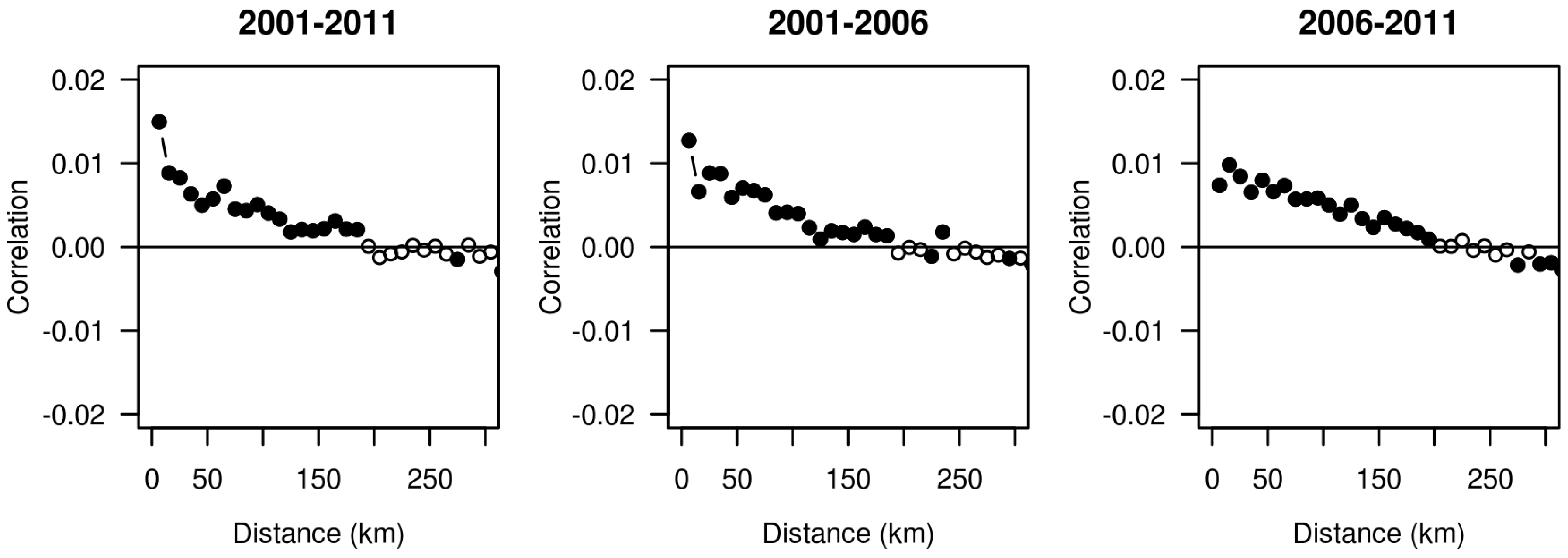
| 2001–2006 | 2006–2011 | 2001–2011 | |
|---|---|---|---|
| Tree complexity | 5 | 3 | 1 |
| Learning rate | 0.0005 | 0.005 | 0.0005 |
| Number of trees | 9150 | 5300 | 8700 |
| CV r | 0.213 | 0.136 | 0.263 |
| CV r2 | 0.045 | 0.018 | 0.069 |
| Training r | 0.374 | 0.296 | 0.358 |
| Training r2 | 0.140 | 0.088 | 0.128 |
| Mean total deviance | 0.032 | 0.018 | 0.046 |
| Mean residual deviance | 0.019 | 0.012 | 0.028 |
| CV standard error | 0.015 | 0.022 | 0.018 |
| Estimated CV deviance | 0.021 | 0.014 | 0.030 |
| Estimated CV deviance standard error | 0.000416 | 0.000388 | 0.000678 |
© 2016 by the authors; licensee MDPI, Basel, Switzerland. This article is an open access article distributed under the terms and conditions of the Creative Commons Attribution (CC-BY) license (http://creativecommons.org/licenses/by/4.0/).
Share and Cite
Thorn, A.M.; Thompson, J.R.; Plisinski, J.S. Patterns and Predictors of Recent Forest Conversion in New England. Land 2016, 5, 30. https://doi.org/10.3390/land5030030
Thorn AM, Thompson JR, Plisinski JS. Patterns and Predictors of Recent Forest Conversion in New England. Land. 2016; 5(3):30. https://doi.org/10.3390/land5030030
Chicago/Turabian StyleThorn, Alexandra M., Jonathan R. Thompson, and Joshua S. Plisinski. 2016. "Patterns and Predictors of Recent Forest Conversion in New England" Land 5, no. 3: 30. https://doi.org/10.3390/land5030030