Article

Identifying Employment Subcenters: The Method of Exponentially Declining Cutoffs

1
Fannie Mae, 4000 Wisconsin Ave NW, Washington, DC 20016, USA
2
Department of Economics, University of California, Riverside, 900 University Avenue, Riverside, CA 92521, USA
3
Nova School of Business and Economics, Universidade Nova de Lisboa, Lisbon 1099-032, Portugal
*
Author to whom correspondence should be addressed.
Submission received: 20 December 2016 / Accepted: 21 February 2017 / Published: 1 March 2017

Abstract

:
The standard method of identifying subcenters is due to Giuliano and Small. While simple, robust and easy to apply, because it uses absolute employment density and employment cutoffs, it identifies “too few” subcenters at the metropolitan periphery. This paper presents a straightforward modification to this method aimed at remedying this weakness. The modification entails using cutoffs that decline exponentially with distance from the metropolitan center, thereby giving consideration to the employment density of a location relative to that of its locality. In urban studies, there is a long history of estimating employment density “gradients”, the exponential rate at which employment density declines with distance from the metropolitan center. These density gradients differ substantially across metropolitan areas and across time for a particular metropolitan area. Applying our method to Los Angeles, Calgary and Paris, we have found that using cutoffs that decline exponentially at one-half the estimated density gradients achieves an appealing balance between subcenters identified close to the metropolitan center and those identified at the metropolitan periphery. Many other methods of subcenter identification have been proposed that use sophisticated econometric procedures. Our method should appeal to practitioners who are looking for a simple method to apply.

1. Introduction

There is a vast literature that aims to describe metropolitan spatial structure. Since metropolitan spatial structures are so complex and diverse, it is not surprising that many different approaches have been applied, each providing a different filter through which to extract some order and structure from this spatial complexity. Different methods extract different signals, each of which provides useful information in some contexts. The most obvious context in which such ordered description is useful is transportation planning; others include land use planning and the location of public facilities.
One of the main approaches to describing metropolitan spatial structure is subcenter identification. The foundational paper in this literature is Giuliano and Small (GS) [1], which lays out a method of employment subcenter identification based on absolute employment and absolute employment density (hereafter the GS method) and applies it to the Greater Los Angeles area. When the Planning Department at the Southern California Association of Governments (SCAG) extended the application of the GS method with high cutoffs (GS(20,20), which is explained later) to the entire Greater Los Angeles area, it found that four employment subcenters were identified in Orange County, but none in the three peripheral counties, Riverside, San Bernardino and Ventura, which at the time had a combined population of over four million. The Department posed the question: How can the GS method be extended to identify peripheral, as well as central subcenters? Broadly, the answer is clear. In defining a subcenter, consideration should be given not only to absolute employment and absolute employment density within an area, but also to the area’s employment and employment density relative to those of proximate areas. This paper explores a simple extension of the GS method that provides one way of making this idea operational.
The extension is based on a conceptualization of metropolitan spatial structure that draws on the monocentric city model (Alonso [2]; Mills [3]; and Muth [4]), whose inspiration was the evolution in the spatial structure of the North American city. In 1900, North American cities had a dense central business district (CBD) where most primary employment was located, surrounded by a residential hinterland connected to the central city by radial transportation corridors. In the 20th century, with growth in population and per capita income, the major cities evolved into metropolitan areas, and technological improvements, particularly those related to motorized vehicles, caused transportation costs to fall. The results were spatial expansion and decentralization. Residential decentralization occurred first, followed by employment decentralization. The same forces of spatial agglomeration responsible for CBDs applied to suburban employment, leading to the creation of suburban subcenters. To describe the evolving metropolitan spatial structure, starting in the 1950s, urban economists estimated population density gradients, the proportional/exponential rate at which population falls with distance from the city center, and starting in the 1970s, they estimated employment density gradients.
In our method, employment subcenters within a particular metropolitan area are identified by applying the high GS employment and employment density cutoffs at the CBD, but adjusting them downward according to distance to the CBD. We actually present two related methods. In the first, the method of exponentially declining cutoffs (EDC), the exponential rate at which the cutoffs decline with distance is specified exogenously; in the second, the method of density-gradient-related cutoffs (DGC), the exponential rate is some fraction of the particular metropolitan area’s employment density gradient. With a fraction of zero, the DGC method reduces to the GS method. With a fraction of one, the exponential rate at which cutoffs decline with distance equals the employment density gradient, so that subcenters in a locality are identified according to employment density relative to the fitted employment density (more specifically the central cutoff density adjusted downward according to the estimated density gradient) there. The size of this fraction can therefore be interpreted as the weight given to relative compared to absolute employment and employment density in the identification of employment subcenters. For the three metropolitan areas that we investigate, Los Angeles, Calgary and Paris, we find that having the cutoffs decline exponentially at a rate equal to one-half of the respective employment density gradients identifies respective sets of employment subcenters that achieve a balance between central and peripheral employment subcenters and conform well to at least our intuition. The fraction one-half is appealing since it gives equal weight to absolute and relative measures of employment and employment density in the definition of an employment subcenter.
The literature contains many more sophisticated methods of subcenter identification. The principal virtue of ours is that, in contrast to the more sophisticated methods, it is simple to understand and apply. Since it is inspired by the evolution of spatial structure in North American cities, our method of subcenter identification may be better suited to North America than to Europe, where historical cities, towns and villages have coalesced into metropolitan areas.
Later in the paper, we shall discuss how our method might be extended to identify other types of subcenters and how our extended method might be applied in some planning contexts. In the course of our discussion, we shall mention relevant papers from the literature, but shall not attempt a comprehensive literature review and shall compare the results of our method only to Redfearn’s [5] for the Los Angeles CMSA.

2. Identifying Employment Subcenters

The Method of Exponentially Declining Cutoffs

It is standard to use the Giuliano–Small [1] method to identify employment subcenters. A subcenter is defined to be a set of contiguous zones, each of which has an employment density of at least D ̲ employees/unit area and which together have a total employment of at least E ̲ . The word “contiguous” is not without ambiguity. Two standard types of contiguity are rook contiguity and queen contiguity. Two zones are rook contiguous if they share a common border of finite length while two zones are queen contiguous if they share only a common point. Giuliano and Small defined two zones to be contiguous if they share a common border of at least a quarter of a mile, a form of rook contiguity, while in this paper we use queen contiguity. We refer to D ̲ as the employment density cutoff and to E ̲ as the total employment cutoff. Further, we denote this method of identifying subcenters as GS( D ̲ , e ̲ ), where e ̲ = E ̲ 1000 ; thus, for example, GS(49.42, 20) denotes the Giuliano–Small method when D ̲ = 49.42 employees per hectare and e ̲ = 20 (so that E ̲ = 20,000 employees) are used as the cutoffs. Giuliano and Small used employment density cutoffs of 20 employees per acre. In this paper, we employ metric units throughout using a density cutoff of 49.42 employees per hectare, which is the metric equivalent of 20 employees per acre.
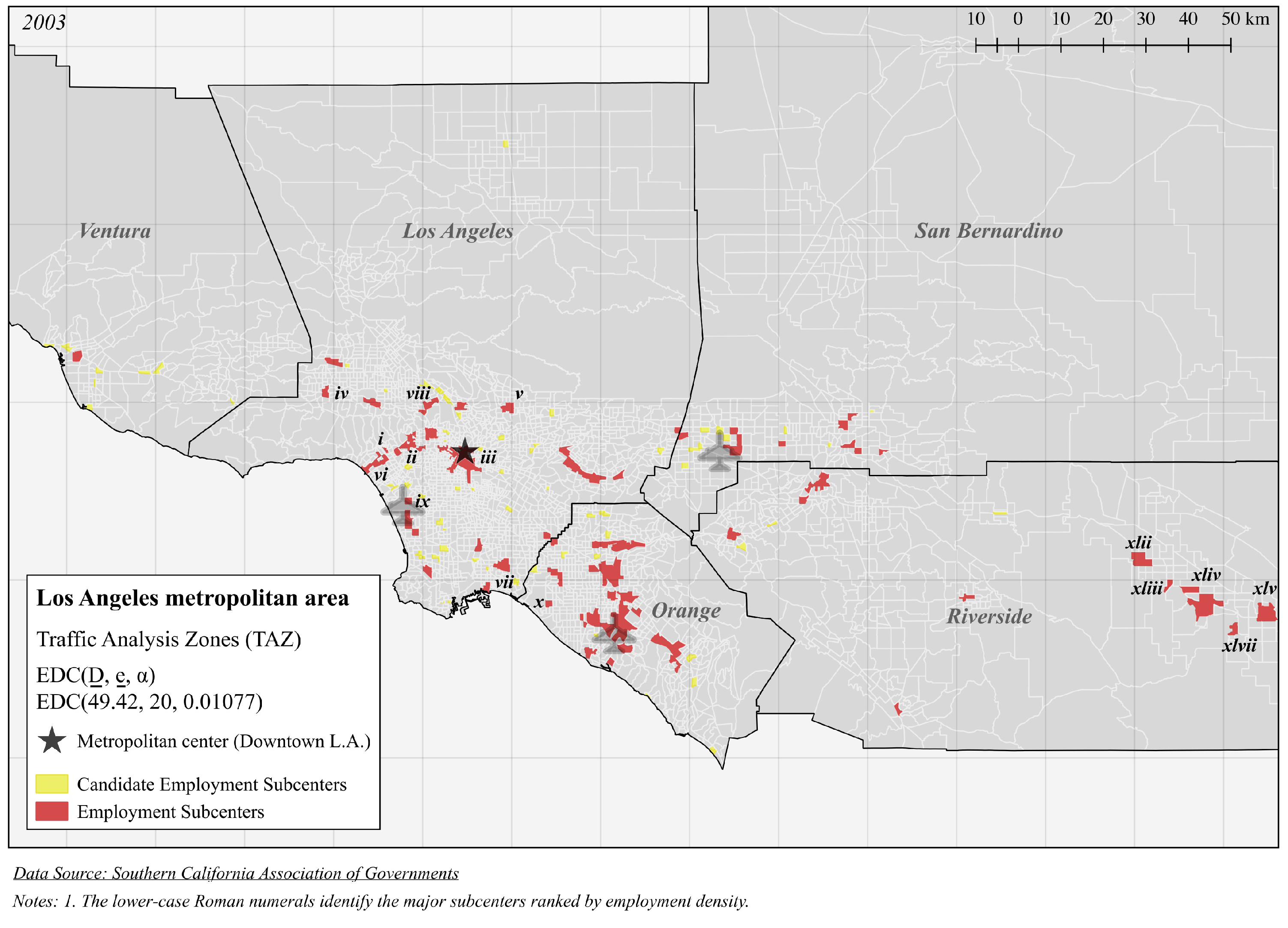
Figure 1 displays a map of the employment subcenters in the Los Angeles metropolitan area identified by applying GS(49.42, 20) to employment data for the 3999 traffic analysis zones (TAZs) in 2003. In that year, the Los Angeles metropolitan area had an area of 21,759,397 hectares, a total employment of 7,478,925 and a total population of 17,438,806. The Census Bureau defines the Los Angeles-Long Beach-Santa Ana Metropolitan Statistical Area to include Los Angeles and Orange Counties and the Los Angeles-Long Beach-Riverside Combined Statistic Area or the Greater Los Angeles Area to include Los Angeles, Orange, Riverside, San Bernardino and Ventura Counties. When we use the term “Los Angeles metropolitan area”, using small letters for metropolitan area, we are referring to the Greater Los Angeles Area. Appendix Table A1 lists data sources, summary statistics and units of measurement for the metropolitan areas of Los Angeles, Calgary and Paris.
One noteworthy feature, on which this paper focuses is that according to GS(49.42, 20) in 2003, there were no subcenters in Riverside, San Bernardino or Ventura Counties, even though the counties had 2000 Census populations of 1,545,387, 1,709,434 and 753,197, respectively. From the GS(49.42, 20) perspective, these three counties appear to be a vast, undifferentiated wasteland. Though this may be the perception of many Los Angelenos, residents of each of the three peripheral counties would assert that, to the contrary, there is a well-recognized set of employment subcenters in their county. That GS(49.42, 20) does not identify peripheral subcenters is a natural consequence of defining a subcenter based on absolute employment and absolute employment density.
The aim of this paper is to present an alternative method of identifying subcenters that identifies peripheral, as well as central, subcenters. An obvious approach is to identify subcenters on the basis of employment density relative to that of the surrounding area and of total employment relative to that of the surrounding area. The major problem with this approach is that it identifies “too many” subcenters at the metropolitan periphery; in the context of Los Angeles, it identifies most desert communities as subcenters. Clearly, what is needed is some intermediate method that combines absolute and relative employment density and total employment. Many such methods can be devised.
This paper explores a method that is particularly easy to understand and apply, is a simple extension of the GS method and, at least for the three illustrative metropolitan areas we consider, gives results that accord well with what the metropolitan area’s residents would identify as its major subcenters. The general approach entails having the employment density and total employment cutoffs fall off in some systematic way with distance from the metropolitan center. In our method, the employment density and total employment cutoffs fall off exponentially with distance from the metropolitan center. There is a long history in urban studies of estimating employment density gradients, the exponential rate at which employment density falls off with distance from the metropolitan center for a specific metropolitan area. Kemper and Schmenner [6] provides a history of thought of population and employment density gradients. According to them, the concept of a population density gradient was popularized by Clark [7]. Muth [4] provided economic microfoundations for the concept. The density gradient concept was first extended to employment by Niedercorn [8]. The particular method we investigate employs metropolitan-specific cutoffs that fall off exponentially at some fraction, θ, of the employment density gradient estimated for the metropolitan area. θ can be interpreted as the weight given to relative compared to absolute employment density and employment in identifying subcenters. For our three illustrative metropolitan areas, Los Angeles, Calgary and Paris, θ = 0.5 gives results that accord well with local knowledge. This is appealing since it means that our approach works well when giving equal weight to relative and absolute employment densities and employment levels.
We do not think that there is a right method to identify employment (or other types of) subcenters, nor therefore that our method is superior to other methods. It would be straightforward to apply the GS method, and indeed our method, to identify other types of subcenters, such as retail, residential, and trip subcenters. We elaborate on this point in Section 5. Different methods are appropriate for people with different levels of statistical training and for different purposes. Our method is appropriate for students and practitioners who have only basic statistical training and wish to undertake a “first-pass” analysis that identifies peripheral as well as central subcenters. For this purpose, we provide a hard copy of the documented Subcenter Identification Algorithm R Script for our method in the Appendix, that would make it straightforward to apply to other metropolitan areas on the basis of employment data available at the census tract or TAZ level. There are many other methods that are considerably more sophisticated in terms of both their statistical methods employed and their conceptual foundations (Cladera et al. [9]; Craig and Ng [10]; Gilli [11]; Giuliano et al. [12]; McMillen [13,14]; Marmelejo et al. [15]; and Redfearn [5]). Such methods would be more appropriate for academic researchers, more technical planning practitioners, and for more refined analysis.
Section 3 introduces our method with an exogenous employment density gradient and illustrates its application to a hypothetical city, and then to the Los Angeles metropolitan area in 2003. Section 4 introduces and discusses a refinement of the method, in which, for a particular metropolitan area, the cutoff employment density gradient is a fraction θ of the estimated employment density gradient for that metropolitan area, and illustrates its application to the Los Angeles, Calgary and Paris metropolitan areas. With θ = 0 , our method reduces to the GS method, in which the same density cutoffs are applied throughout the metropolitan area, and which therefore is based on absolute employment density and employment level; with θ = 1 , our method is based on relative employment density and employment level; and with θ = 0.5 , our method gives equal weighting to absolute and relative employment density and employment level. Section 5 discusses technical issues and possible uses of our method, and Section 6 concludes. The Appendix provides the data sources and summary statistics for each metropolitan area, tables of subcenter level characteristics for those identified by the method and shown in the maps, higher resolution maps highlighting the individual counties of Los Angeles, and an algorithm developed under the R language for identifying subcenters according to our method, as well as instructions on how to combine the elements for actual application to a different metropolitan area.

3. The Method of Exponentially Declining Cutoffs

As in the Giuliano–Small method, an employment subcenter is a set of contiguous zones, each of which has an employment density that exceeds the cutoff employment density for that zone and such that its total employment exceeds the cutoff total employment for its constituent zones. The method of exponentially declining cutoffs differs from the Giuliano–Small method in two respects. First and more importantly, the cutoffs fall off exponentially with distance from the metropolitan center, which is defined as the centroid of the zone with the highest employment density. Second, we employ a definition of contiguity that is slightly different and easier to apply than the definition used in Giuliano–Small.
We employ the following notation:
Demployment density
Etotal employment
αcutoff gradient
x(Euclidean) distance from the metropolitan center
zzonal index
C Z set of candidate zones
C S set of candidate subcenters
The method of exponentially declining cutoffs has five steps for determining subcenters.
  • Determine the cutoff level of employment density for each zone.
    D z ̲ = D ̲ e α x z or ln D z ̲ = ln D ̲ α x z
    where D z ̲ is the cutoff employment density in zone z, D ̲ is the cutoff employment density at the metropolitan center, x z is the distance between the zone centroid and the metropolitan center and α is the cutoff gradient, the proportional rate of decline of the cutoff with distance (e.g., 20% per kilometer). In other words, the cutoff employment density in zone z equals the cutoff employment density at the metropolitan center, adjusted downward as a function of distance from the metropolitan center according to e α x z .
  • Determine the set of candidate zones.
    A candidate zone is a zone whose actual employment density, D z , exceeds the cutoff employment density for that zone. Denoting by C Z the set of candidate zones,
    z C Z iff D z > D z ̲ .
    In other words, a zone is a candidate zone if and only if its employment density exceeds its cutoff employment density based on distance from the metropolitan center.
  • Group zones into candidate subcenters.
    A candidate subcenter is a set of candidate zones that form a contiguous set and are contiguous to no other candidate zones. By definition, candidate subcenters are mutually exclusive (i.e., a candidate zone cannot be in more than one candidate subcenter). Let s index the candidate subcenters and C S denote the set of candidate subcenters. By definition s C S .
  • Determine the cutoff level of total employment for each candidate subcenter.
    E s ̲ = E ̲ e α x s ,
    where E s ̲ is cutoff total employment in candidate subcenter s, E ̲ is cutoff total employment at the metropolitan center and x s is the employment-weighted distance between the candidate subcenter and the metropolitan center. In particular, where n is the number of zones in candidate subcenter s, x z ( z = 1 , , n ) is the distance between zone z and the metropolitan center, and E z is the total employment of zone z, x s is defined as Σ E z x z Σ E z . In other words, the cutoff level of total employment for a candidate subcenter equals the cutoff level of total employment for a subcenter at the metropolitan center, adjusted downward as a function of the distance from the employment-weighted centroid of the candidate subcenter to the metropolitan center according to e α x s .
  • Determine the set of subcenters.
    Where S is the set of (proper) subcenters and E s is the total employment of candidate subcenter s,
    s S iff E s > E s ̲
    In other words, a candidate subcenter is a (proper) subcenter if and only if its total employment exceeds its total employment cutoff based on distance from the metropolitan center.
We denote this method of exponentially declining cutoffs by EDC( D ̲ , e ̲ , α).
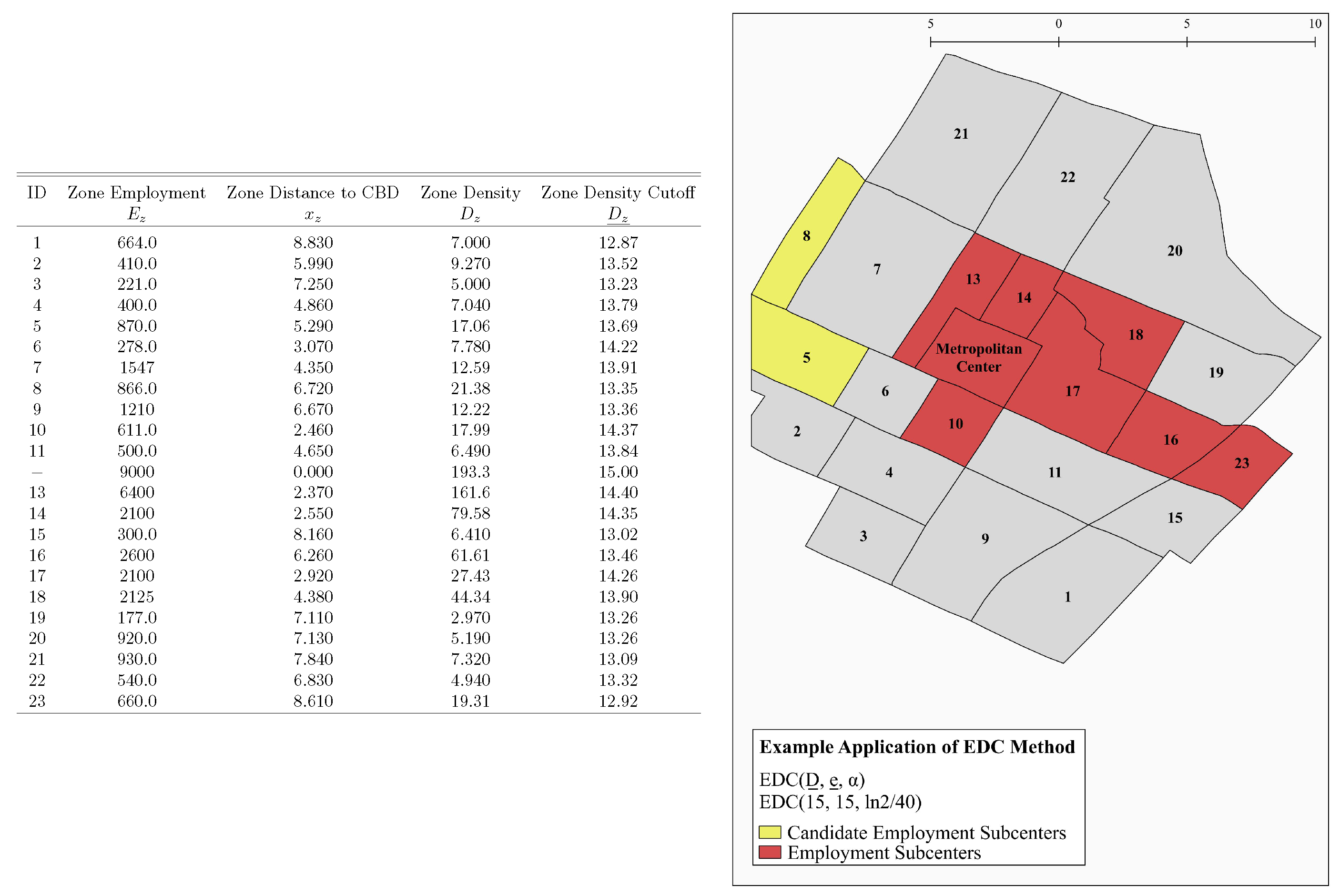
Figure 2 illustrates an application of this method in an example with D ̲ = 15 , e ̲ = 15 and α = l n 2 40 = 0.01732 . The hypothetical metropolitan area contains 23 zones. The table lists each zone’s employment, employment density, cutoff employment density based on the distance of the zone centroid from the metropolitan center, and distance of the zone centroid from the metropolitan center ( x z ). Zone z’s cutoff employment density is D ̲ e α x z . The cutoff gradient is chosen so that the cutoff employment density halves every 40 distance units from the metropolitan center. To see this, solve the α for which D z / D ̲ = e α x z = 0.5 when x z = 40 : e α ( 40 ) = 0.5 . Taking the natural logarithm of both sides yields 40 α = l n 0.5 , so that α = l n ( 0.5 ) 40 = l n 2 40 . At a distance of 5 units for example, the cutoff employment is 15 · e x p { ( l n 2 40 ) 5 } = 13.76 .
In the example, there are ten zones whose employment density exceeds the distance-dependent employment density cutoffs, zones 5, 8, the metropolitan center, 10, 13, 14, 16, 17, 18, and 23, and which are therefore candidate zones. These zones form two mutually exclusive contiguous sets, each of which is a candidate subcenter. The first candidate subcenter (shown as the yellow area) comprises zones 5 and 8, and the second candidate subcenter (shown as the red area) comprises the metropolitan center, 10, 13, 14, 16, 17, 18, and 23. A candidate subcenter is a (proper) subcenter iff its total employment exceeds its cutoff total employment, calculated as E ̲ e α x s , where E ̲ = 15,000 is the total employment cutoff at the metropolitan center, and x s is the employment-weighted distance between the candidate subcenter and the metropolitan center. In the example, the first candidate subcenter is not a proper subcenter, while the second candidate subcenter is a proper subcenter.
When we first started work on this paper, we used Anglo-Saxon units. Our initial somewhat educated guess was that we would get a good balance between central and peripheral subcenters with cutoffs that halved every 40 miles. In metric units, this corresponds to α = 0.01077 . Figure 3 illustrates the set of employment subcenters determined by applying EDC(49.42, 20, 0.01077) to the 3999 TAZs in the Greater Los Angeles metropolitan area in 2003.
The most noteworthy feature of the figure is that subcenters appear in the wasteland: 11 subcenters emerge in Riverside County, 5 in San Bernardino County and 1 in Ventura County. With one qualification, these subcenters are what residents would identify as the major employment centers in their counties. The qualification concerns the Palm Spring area, which runs along the Coachella Valley from Palm Springs to Indio, and includes subcenters xlii to xlv in Figure 3. First, the Palm Springs area is arguably part of the Greater Los Angeles metropolitan area only by definition and should properly be viewed as a separate metropolitan area. In the United States, metropolitan areas are defined on the basis of their constituent counties. The distance from Corona, which is at the west end of Riverside County, to Blythe, which is at the east end, is 291.6 km.
Second, most Riverside County residents would view the Palm Springs area as a single employment subcenter. The reason our method identifies it as having several subcenters derives from its narrowness, which results from a combination of topography and microclimate. Predominantly commercial zones alternate with predominantly residential zones. Our reaction is that any simple method of subcenter identification will generate anomalies that are best dealt with on ad hoc basis. Our method identifies 47 subcenters in the entire metro area. In addition to those in the peripheral counties, it identifies 19 subcenters in Los Angeles County, nine in Orange County and two subcenters overlapping between counties, the first between Los Angeles and San Bernardino and the second between Los Angeles and Orange County.
Redfearn [5] identifies subcenters in the Los Angeles CMSA, which comprises Los Angeles and Orange Counties, for the year 2000 using census tracts as zones. His subcenter identification procedure is considerably more sophisticated than ours but like ours considers relative employment densities. It is of interest to compare the subcenters he identified with those that we identified in the Los Angeles CMSA. Redfearn identifies 41 (statistically significant) employment subcenters, which are shown in Figure 9 of his paper. We obtained 30 employment subcenters (the 19 in Los Angeles County, the nine in Orange County, the one that overlaps Los Angeles and Orange County and the one that overlaps Los Angeles and San Bernardino County), which are shown in Figure 3 of our paper. To our eyes at least, there is a close correspondence between the two sets of subcenters identified. We have identified four sources of the differences. First, Redfearn’s zones are census tracts, whereas ours are TAZs; and second, Redfearn’s data are for the year 2000, whereas ours are for the year 2003. Neither of these differences appears important. The third is that Redfearn identifies subcenters based on (smoothed) relative employment density, not including total employment cutoffs, which by itself would result in Redfearn’s method identifying more subcenters than ours. The fourth difference is that Redfearn’s method entails spatial smoothing, which results in some subcenters identified by our method merging along freeway corridors, which by itself would result in Redfearn’s method identifying fewer subcenters than ours.
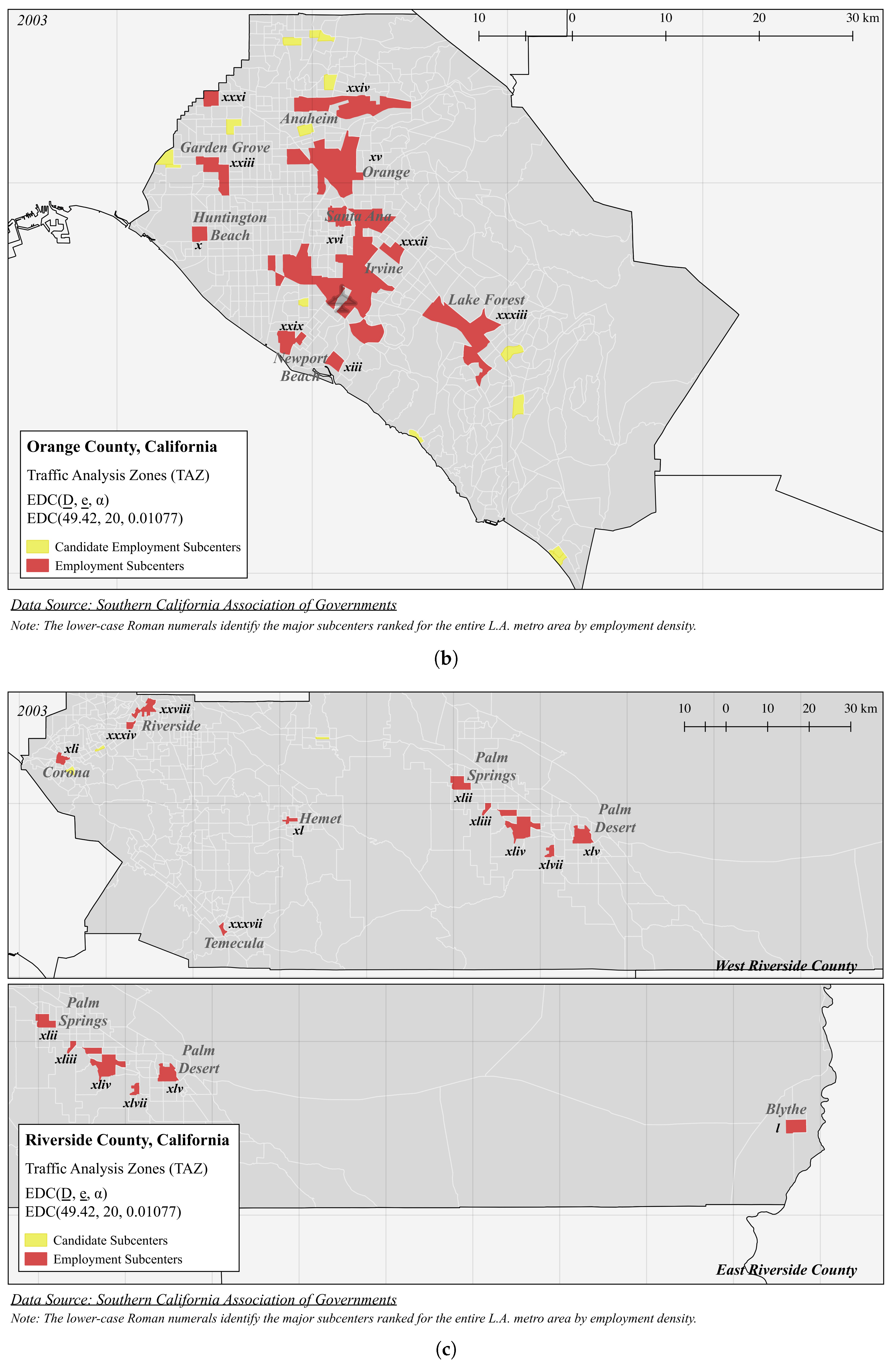
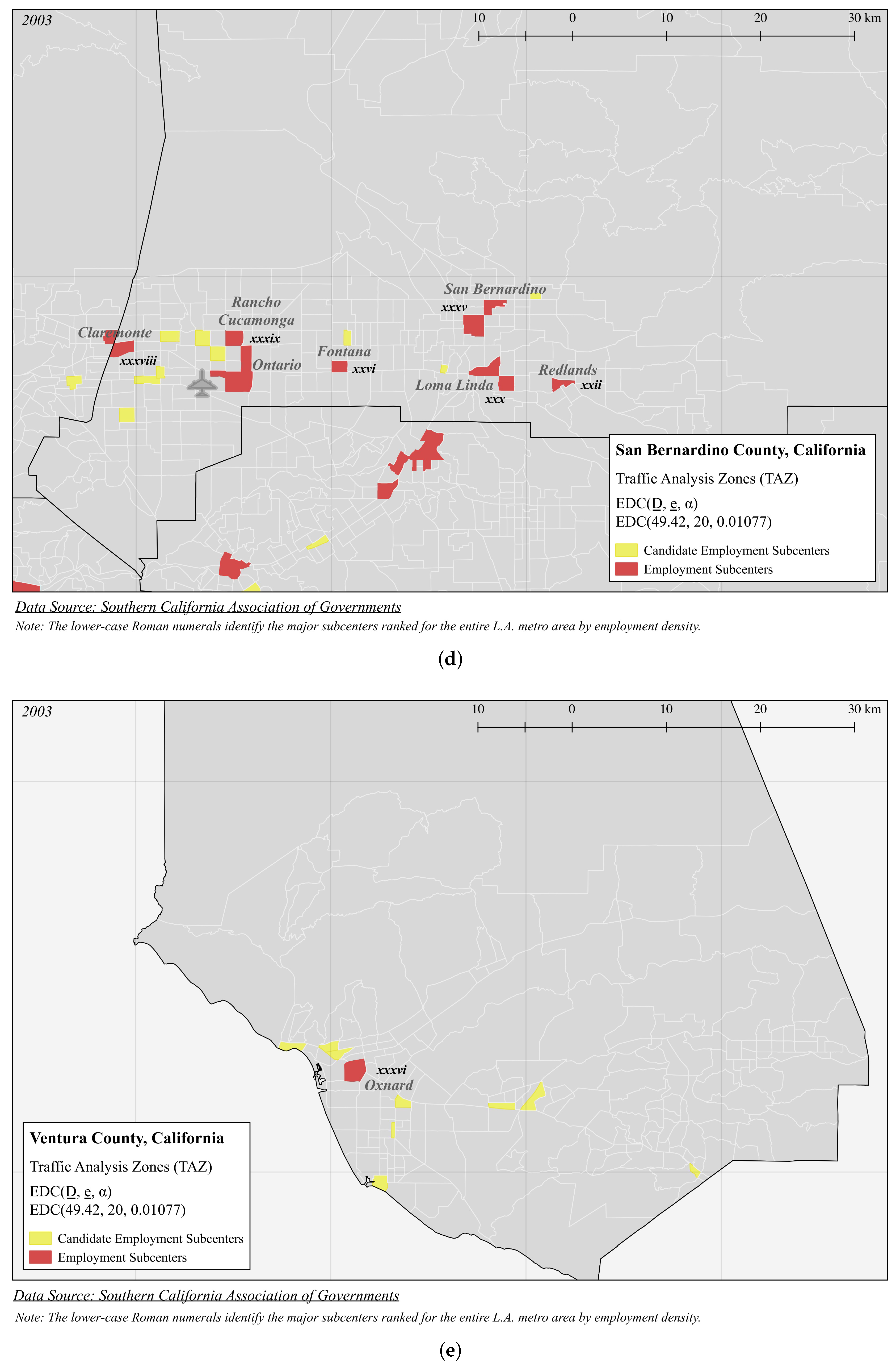
The Appendix displays separate maps of the subcenters identified by applying EDC(49.42, 20, 0.0177) for each of the area’s constituent counties, identifying the major city associated with each subcenter. In each map, the top ten subcenters, as ranked by their employment density, are highlighted with further information for each in the appendix.
The EDC procedure is based on four assumptions, and the results of its application are only as good as the soundness of these assumptions. The first is that cutoff employment density should fall off with distance from the metropolitan center in a spatially symmetric fashion. The second is that cutoff employment density should fall off exponentially with distance from the metropolitan center. The third is that cutoff total employment in subcenters should fall off exponentially with distance from the metropolitan center at the same rate as cutoff employment density. Additionally, the fourth is that the assumed cutoff gradient (for both employment density and total subcenter employment) achieves the best balance between identifying central and peripheral subcenters.
One way of establishing the soundness of these assumptions is to appeal to the empirical evidence; another is to appeal to theory. Appealing to the empirical evidence is the more persuasive, but the latter may be a defensible alternative where empirical evidence is scant.
The voluminous literature on the estimation of urban employment density gradients assumes that average employment density falls off symmetrically and exponentially from the city center. These assumptions are sufficiently strongly supported by the empirical literature to justify the analogous assumptions with respect to cutoff employment density in the type of first-pass analysis that we have in mind. More sophisticated methods of subcenter identification, such as that in McMillen [13], relax these two assumptions. The third assumption is, to our knowledge, untested empirically. The empirical analysis presented later in the paper is broadly consistent with the fourth assumption, but, since it employs a sample size of three (the three metropolitan areas to which we apply our method), this hardly constitutes compelling evidence.
Since the empirical evidence regarding the third and fourth assumptions is weak, we consider theoretical justifications for them. Central place theory, as represented in Christaller [16] and Lösch [17], considers a spatially repeated pattern of a hierarchy of subcenters on a large, homogeneous plain. Now introduce a “pole of attraction” into this space, with the location of the pole being the result of a natural advantage such as a good harbor (“first nature”: Cronon [18]). The pole causes each spatial unit of replication to be compressed and by more the closer is the spatial unit of replication to the pole of attraction. We envision a metropolitan area’s center to be located at this pole of attraction. By itself, this compression does not alter the total employment at each level of hierarchy of subcenters. To achieve this, one may introduce the notion of location potential, whereby a location develops base employment when and only when production is profitable there. Then compression of a spatial unit of replication causes total employment at each level of its hierarchy of subcenters to increase.
Fujita, Krugman, and Mori [19] derive qualitatively the same spatial pattern in a new economic geography model of an isolated line segment with multiple manufacturing industries (in each of which the constituent firms produce differentiated products), a taste for variety, and a growing population. At low levels of population, manufacturing is concentrated in a single center. As population increases, a bifurcation is reached at which a new subcenter emerges when production of one of the manufactured goods there becomes profitable. As population continues to increase, an increasingly rich hierarchy of subcenters develops, with employment at subcenters at each level of the hierarchy increasing with proximity to the center.
These two conceptualizations provide somewhat different rationales for the third assumed empirical regularity. Later we shall be more explicit about the fourth assumption. Roughly, it is supported if employment becomes relatively more spatially concentrated as distance from the metropolitan center increases. One explanatory factor is the indivisibility of road land width; road lane width does not shrink as employment density decreases. A central firm that requires close proximity to the freeway system has many locations to choose between but a peripheral firm has only a few.

4. A Refinement of the Procedure

In this section we propose that the employment density gradient for the entire metropolitan area, which we denote by γ, be pivotal in the choice of α. The employment density gradient gives the “average” proportional rate at which employment density falls off with distance from the metropolitan center. If α is set equal to γ, then a zone is identified as a candidate zone by its employment density relative to the fitted employment density at that distance from the metropolitan center. In this sense, candidate zones are identified by their relative employment densities (more specifically, relative to the fitted employment density at that distance from the metropolitan center). Note that this notion of relative employment density is different from a zone’s employment density relative to the average employment density of proximate zones.
More generally, one can set α = θ γ , where θ measures the weight attached to relative employment density compared to absolute employment density. When θ = 0 , all the weight is attached to absolute employment density, and our method reduces to the corresponding GS method. When θ = 1 , all the weight is attached to employment density relative to the fitted employment density at that distance from the metropolitan center. Values of θ greater than one are possible, but we cannot think of situations where one would want to identify subcenters by having the employment density cutoff fall off at a faster rate with distance from the metropolitan center than the metropolitan area’s employment density gradient. We define DGC( D ̲ , e ̲ , θ; γ) to be the method of density-gradient-related cutoffs. The method is characterized by three parameters, D ̲ , e ̲ , and θ, in addition to a metropolitan area’s estimated employment density gradient.
How should the employment density gradient be estimated? The simple employment density gradient is the estimated value of γ by OLS in the regression equation:
l n D z = c γ x z + u z
where z indexes the zone and u z is the error term [20]. More sophisticated estimates of the employment density function can be obtained by adding other accessibility co-variates, such as distance from the nearest freeway and, in the case of the Los Angeles metropolitan area, distance from the ocean (but not distance from nearby subcenters, since they are endogenous to the procedure), by taking account of spatial correlation in the error term, and by using more flexible functional specifications and non-parametric specifications. For our method, we favor the use of the simple employment density gradient since its estimation follows a simple, standard procedure. In contrast, if non-standard methods were used, different studies would employ different sophisticated methods, which would make comparability of studies for the same metropolitan area more difficult.
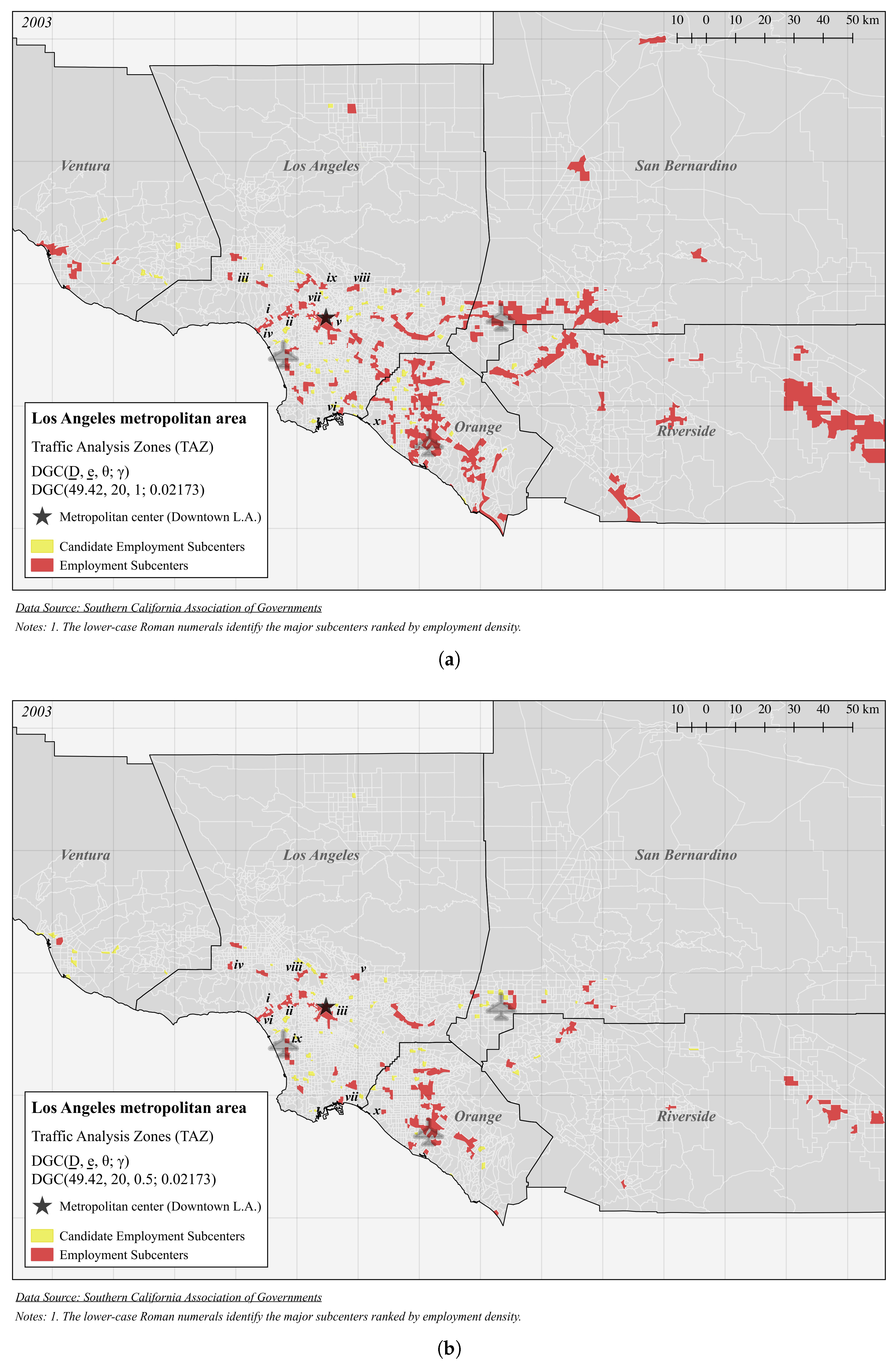
Using TAZs, the estimated value of γ for the Los Angeles metropolitan area in 2003 is 0.02173, which indicates that employment density falls off at a rate of approximately 2.2% per kilometer. Figure 4a shows the subcenters identified according to DGC(49.42, 20, 1; 0.02173), the Giuliano–Small method, but with cutoffs declining exponentially at the rate of the simple employment density gradient. To our eyes, applying the DGC method with θ = 1 to the area identifies too many subcenters, especially at the metropolitan periphery. The reason seems to be that employment is more spatially concentrated at the metropolitan periphery, lying close to the freeways. Figure 4b shows the subcenters identified according to DGC(49.42, 20, 0.5; 0.02173), the Giuliano–Small method, but with the cutoffs declining exponentially at a rate equal to one-half of the simple employment density gradient. The employment subcenters identified using values of θ = 0.5 are very similar to those identified in Figure 3. The reason is that the rate of exponential decay in Figure 3, α = 0.01077 , is very similar to 0.5 times the density gradient of 0.02173. Thus, applying the DGC method to the Los Angeles metropolitan area with equal weight on relative and absolute employment density gives reasonable results, while complete weight on absolute employment density or relative employment density identifies too few or too many subcenters respectively.
To check on the transferability of our procedure, we applied it to two other metropolitan areas, Calgary, Canada, and Paris, France. We chose those two metropolitan areas only because the data for them were readily available, having previously been used by Arnott in other contexts. For these metropolitan areas we consider only the DGC procedure.

4.1. Calgary

Calgary, Canada is a metropolitan area on the immediate eastern side of the Rockies. Since oil was discovered at Leduc, Alberta, in 1947, it has become the center of Canada’s oil and gas industry, and its population has grown at a high average rate. The Calgary census metropolitan area (CMA) includes nine municipalities: 3 cities (Calgary, Airdrie, Chestermere); 1 municipal district (Rocky View County); 3 towns (Cochrane, Crossfield, Irricana); 1 village (Beiseker); and 1 First Nations reserve (Tsuu T’ina Nation 145). In 2011, the population of the Calgary CMA was 1,214,839 of which the City of Calgary itself was 1,096,833, with an additional 21,258 in the Foothills No. 31 municipal district to the south, 3893 in Vulcan County and 8285 in Wheatland County.
We employ exactly the same procedure for Calgary as for Los Angeles, using TAZs, a central employment density cutoff of 49.42 employees per hectare, and a central total employment cutoff of 20,000. The data for Calgary are for the year 2006, when there were 1869 TAZs. At that time the total employment of the CMA was 664,290 and its total land area was 1,383,138 hectares. We apply the procedure to the Calgary metropolitan area, inclusive of the Calgary CMA, the Foothills No. 31 municipal district, and Vulcan and Wheatland Counties. The estimated employment density gradient for Calgary is 0.1139, over five times that of Los Angeles. At first glance, this is surprising since until quite recently Calgary was very much an automobile city. Starting in the mid-1980s, the Calgary metropolitan planning and transportation agencies have been pushing transit-oriented development hard, through aggressive expansion of the LRT network and a soft downtown parking freeze. The high density gradient is explained by the fact that Calgary’s base employment has been dominated by the corporate headquarters of firms in the oil and gas industry, which have been located in the central business district.
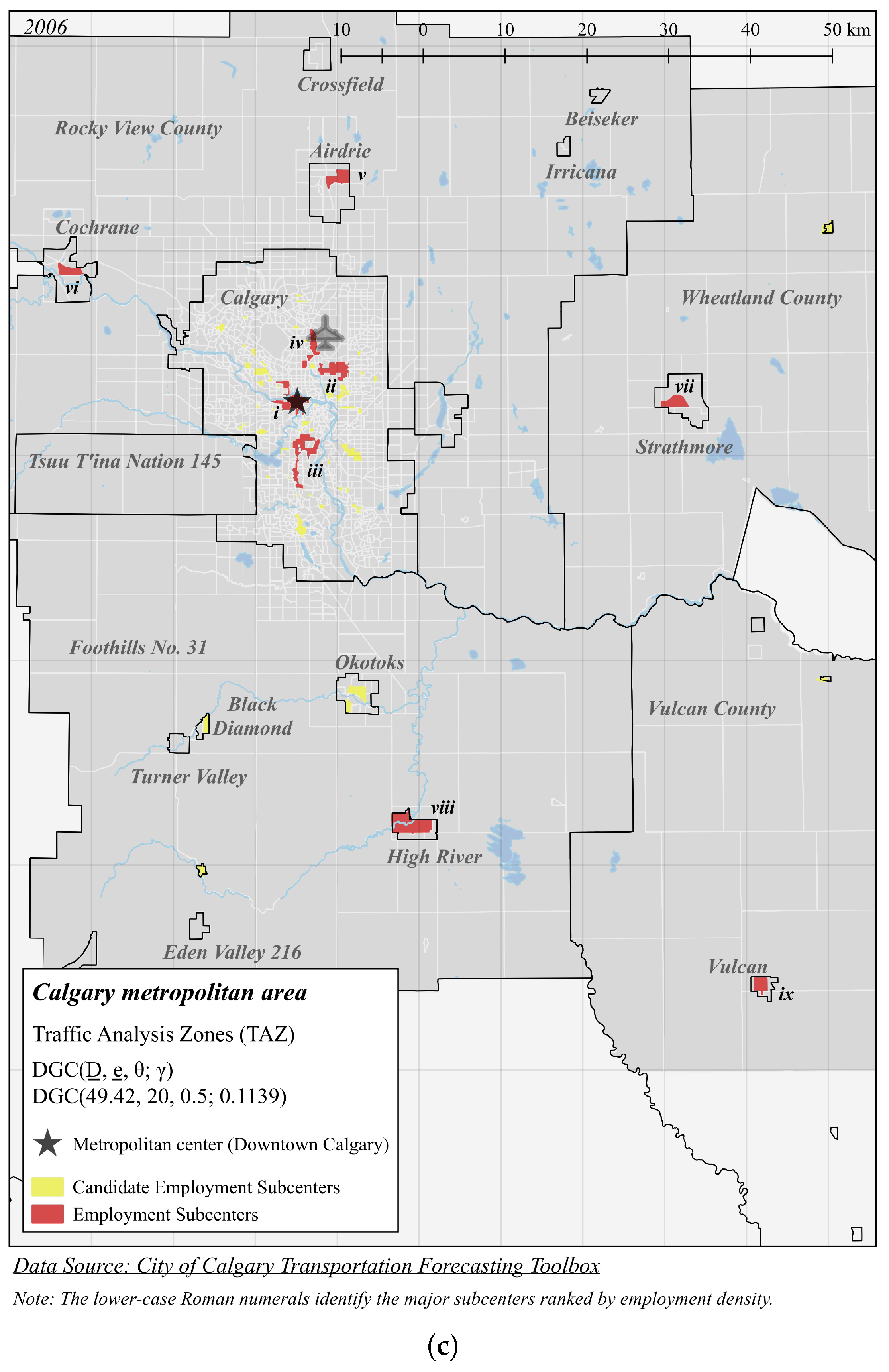
Figure 5 contains three panels. The first, Figure 5a, maps candidate employment subcenters and proper subcenters using DGC(49.42, 20, 0; 0.1139). This is the same as the GS procedure, and consequently identifies subcenters on the basis of absolute employment density and employment. The second, Figure 5b, maps candidate subcenters and proper subcenters using DGC(49.42, 20, 1; 0.1139). This procedure identifies subcenters on the basis of relative employment density and employment. The third, Figure 5c, maps candidate subcenters and proper subcenters using DGC(49.42, 20, 0.5; 0.1139). This procedure places equal weight on absolute and relative employment in the identification of subcenters; as with the Los Angeles metropolitan area, it does this by employing exponentially declining cutoffs that decline at the rate equal to one half the estimated employment density gradient.
As θ increases from zero to one, more employment subcenters are identified, with an increasing proportion away from the downtown core. One might think that the number of subcenters always increases as θ increases since the criteria to become a subcenter are weakened. The number of candidate zones (those that meet the employment density cutoff) does indeed always increase. However, as θ increases the number of candidate subcenters does not always increase since what were previously separate subcenters may meld together.
Under the GS-equivalent specification ( θ = 0 ) of Figure 5a, only two employment subcenters are identified, the downtown core and an area south of the airport. At the opposite extreme with θ = 1 , Figure 5b identifies nine subcenters in the City itself and 15 in the metropolitan hinterland outside the City limits. The latter 15 all started as small entrepôts in Calgary’s agricultural hinterland. Several have subsequently become bedroom communities for Calgary. Figure 5c displays the intermediate case with θ = 0.5 . Four subcenters are identified in the City and five outside the city. They correspond closely to what Calgarians would identify as the area’s employment subcenters. Thus, as with the Los Angeles example, the DGC method with θ = 0.5 achieves a balance between identifying too few and too many subcenters at the urban periphery.

4.2. Paris

Until about 1960, Paris was known for the dominance of central Paris, la ville de Paris or Paris intra muros, within metropolitan Paris (the Île-de-France). Since then the French government has followed a program of decentralization, by building the villes nouvelles in the 1960s, more recently by imposing height and redevelopment restrictions in central Paris and extending the subway system to the suburbs (the RER), and even more recently by decentralizing land use planning. The decentralization of population was followed by the decentralization of employment, to the point where the bulk of commutes are now suburb-to-suburb. See Gilli [11] for a more detailed discussion of the recent evolution of spatial structure in the Île-de-France.
The data for the Paris metropolitan area are for the year 2005. At that time, its population was 11,433,302, its area was 1,206,953 hectares, and its employment was 5,359,731. We employ almost exactly the same procedure for Paris as we did for Los Angeles. The only difference is that the Paris data were collected by commune, of which there are 1299. The employment density gradient calculated for the Île-de-France is 0.08041 which is almost four that for Los Angeles.
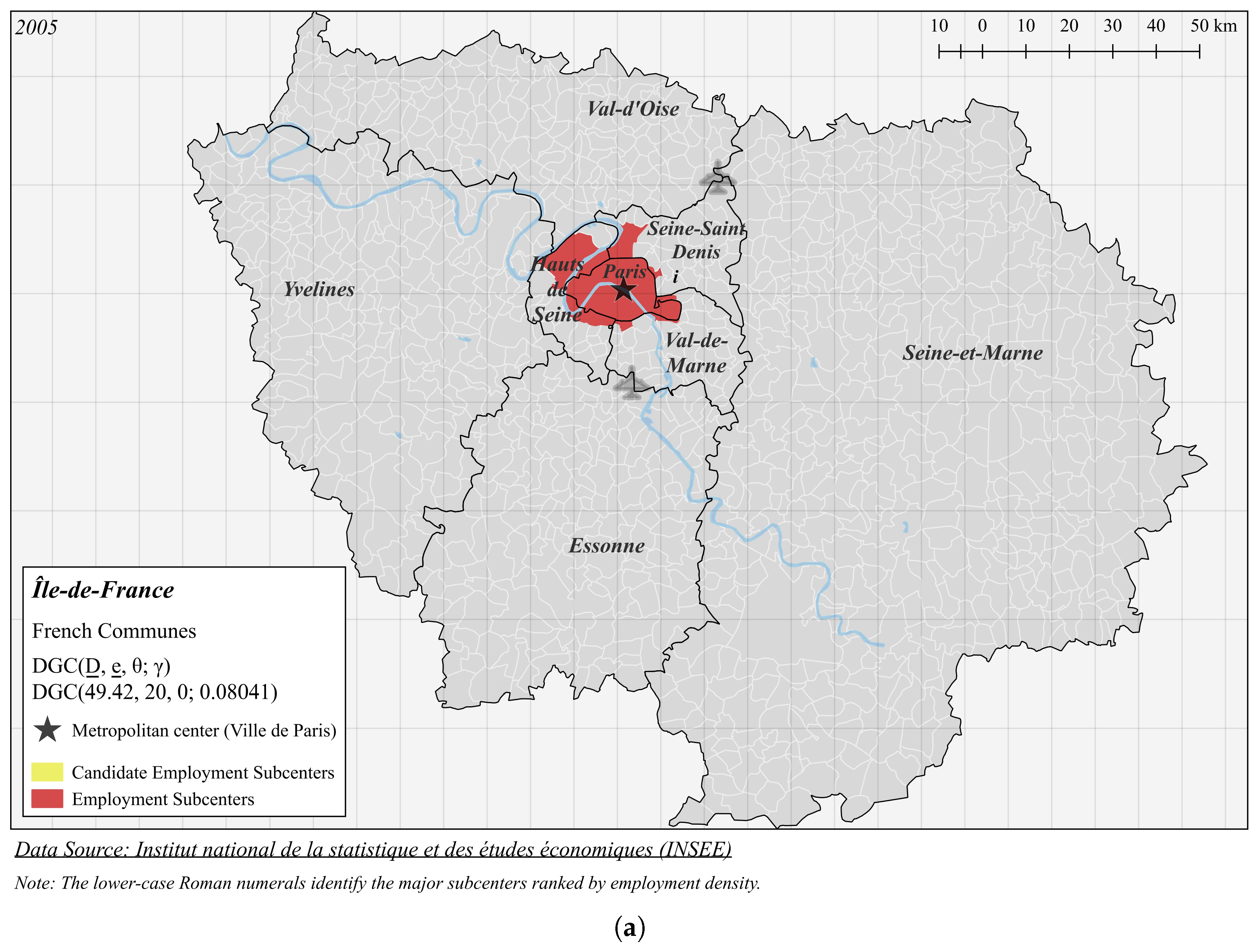
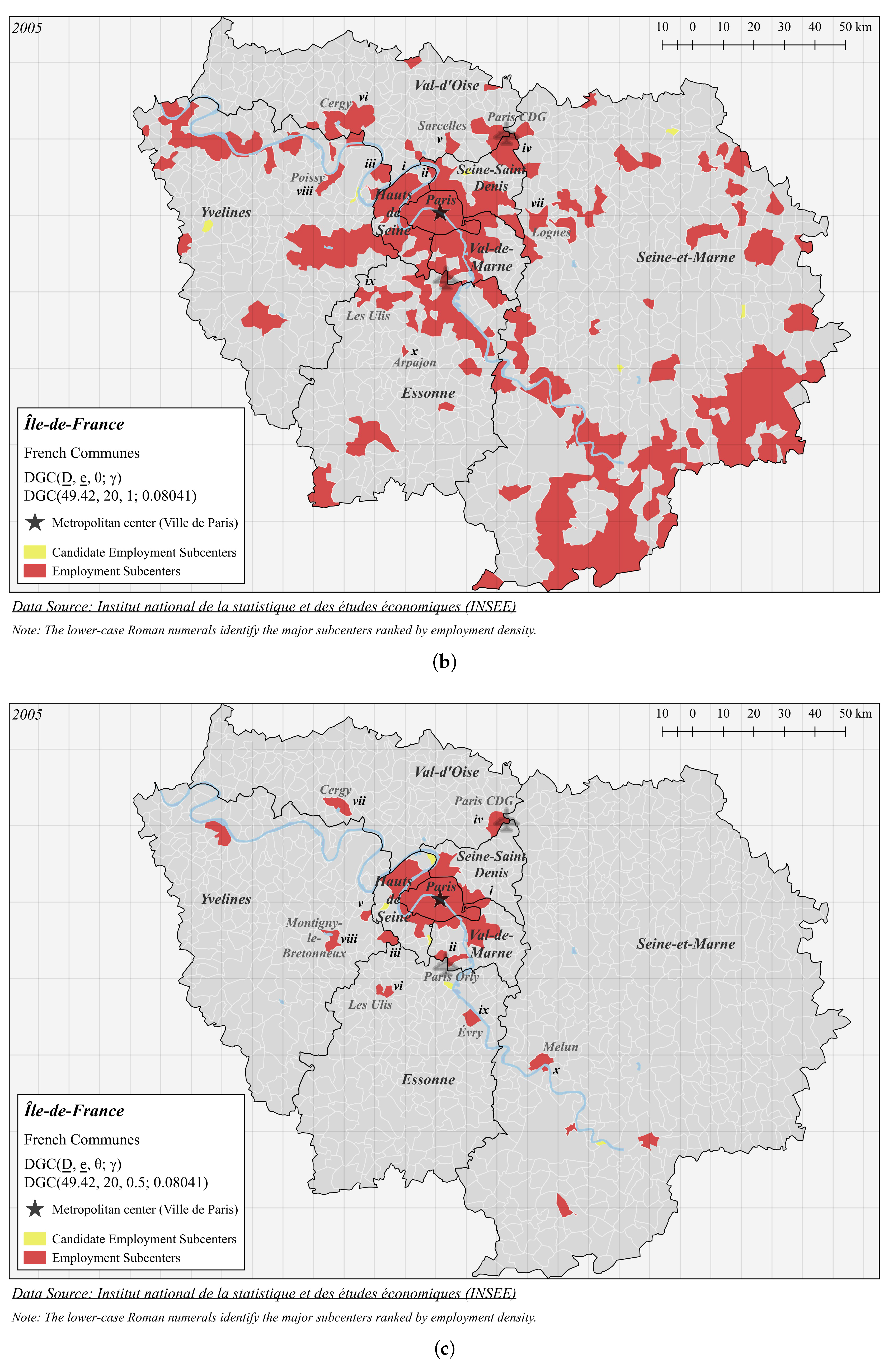
Figure 6 contains three panels. The first, Figure 6a, maps candidate employment subcenters and proper subcenters using DGC(49.42, 20, 0; 0.08041). This is the same as the GS procedure, and consequently identifies subcenters on the basis of absolute employment density and employment. The second, Figure 6b, maps candidate employment subcenters and proper subcenters using DGC(49.42, 20, 1; 0.08041). This procedure identifies subcenters on the basis of relative employment density and employment. The third, Figure 6c, maps candidate employment subcenters and proper subcenters using DGC(49.42, 20, 0.5; 0.08041). This procedure places equal weight on absolute and relative measures in the identification of subcenters. Information on the identified subcenters are in the appendix. In the figure, the labels in black are the names of the départements that together constitute the Île-de-France.
The maps are strongly different from one another. Figure 6a identifies only one employment center, which covers la ville de Paris and several of the communes adjacent to the city center. This reflects the traditional dominance of central Paris in the Paris Region. Figure 6b, in sharp contrast, identifies 49 employment subcenters, with about half bordering on or including the Seine River, which is marked in blue on the map. Also noteworthy is that there are very few candidate subcenters that are not proper subcenters, indicating that most subcenters that meet the employment density cutoff also meet the total employment cutoff. As discussed later, this likely reflects that communes tend to be larger than TAZs. The results displayed in Figure 6c are, of course, in between. There are 14 proper subcenters, with only a handful that are neither airport subcenters nor including or abutting the Seine River.
None of us knows the Île-de-France sufficiently well to assert with confidence that the subcenters identified in Figure 6c accord with what the region’s residents perceive to be the subcenters. However, the spacing between subcenters and the proportion of space occupied by subcenters, suggest that this is so. Thus, it appears that the DGC method with θ = 0.5 achieves a balance between identifying what residents would perceive as too many or too few subcenters, or putting insufficient or excessive weight on absolute size in identifying subcenters.

5. Discussion

There is much to be said for the GS method of employment subcenter identification. It is intuitive, easy to implement, and robust. There is also much to be said for continuing to use the standard method, whatever it is, since it facilitates comparison of results across time and metropolitan areas. Since it is not difficult to come up with methods that are superior to the GS method in some respects (see, for example, Giuliano et al., [12], McMillen [13], Redfearn [5]), there is also the danger of method proliferation if alternative methods start to be used, which would compromise the comparability of results across studies. Thus, an alternative method needs a strong justification to be considered.
In this paper we have put forward an alternative method of employment subcenter identification, the method of exponentially declining cutoffs (EDC), and a refinement of it, the method of density-gradient-related cutoffs (DGC). Both methods generalize the GS method by applying employment density and employment cutoffs that fall off exponentially with distance from the metropolitan center, and have the GS method as a limiting case. The most obvious justification for our method is straightforward. Being based on absolute employment density and absolute total employment, the GS method may fail to identify important subcenters in the suburbs and exurbs. For example, applying the GS(49.42, 20) method to 2003 data for the Los Angeles metropolitan area identifies no subcenters at all in the peripheral counties, which at the time had a combined population of over four million. Thus, application of the GS method in this context results in the false perception that the periphery of the Los Angeles metropolitan area is a vast undifferentiated wasteland.
The methods we propose have employment density and total employment cutoffs that fall off exponentially with distance from the metropolitan center. In the EDC method, for a particular metropolitan area, the exponential rate at which the cutoffs fall off with distance from the metropolitan center, α, is chosen to achieve what the user perceives to be an appealing balance between central and peripheral employment centers for that metropolitan area. In the DGC method, for a particular metropolitan area, the exponential rate at which the cutoffs fall off with distance from the metropolitan center is some fraction, θ, of the simple employment density gradient estimated for that metropolitan area, γ, and θ is chosen to achieve what the user perceives to be an appealing balance between central and peripheral subcenters. θ is the weight attached to relative compared to absolute cutoffs; with θ = 1 , the cutoffs at a location are determined relative to the fitted employment density at that location; with θ = 0 , the method is based on absolute cutoffs and is essentially identical to the GS method. For the three metropolitan areas that we investigated, a balance between central and peripheral employment subcenters was achieved with a value of θ = 0.5 , which has the neat interpretation of providing equal weighting to absolute and relative employment density in the choice of the location-dependent cutoffs.
One may reasonably argue that there are other methods of extending the GS method to identify peripheral subcenters that are simpler than either the EDC or DGC methods. For Los Angeles, we experimented with other methods. The most obvious is to lower the cutoffs. As the cutoffs are lowered, the area of land in subcenters increases. Peripheral subcenters are identified, but the central subcenters become larger and some meld together, blurring their identity. For example, in the Los Angeles metropolitan area, the entire Wilshire Corridor, which extends all the way from downtown Los Angeles to the coast, a distance of 15 to 20 miles, becomes one large subcenter, which accords neither with the perception of residents nor with the skyline. Another method is to apply one pair of higher cutoffs to central areas and another pair of lower cutoffs to peripheral areas. One problem with this method is that the division between central and peripheral areas is arbitrary. Another is that the “wasteland” problem reemerges but at a reduced spatial scale. Exurbia becomes a wasteland from the perspective of the suburbs, and the central areas that are furthest from the metropolitan center may appear to be wasteland too.
Since the employment density gradient differs strongly across metropolitan areas (see Glaeser and Kahn [21]), we advocate the use of our methods for identifying subcenters within a particular metropolitan area but not for the comparison of subcenters across metropolitan areas.
We are agnostic concerning whether the EDC or the DGC method be employed. Both entail an element of arbitrariness in the choice of the exponential rate of decline of the employment density and total employment cutoffs. In the EDC method, this comes through the choice of α, and in the DGC method through the choice of θ. The essential difference between the two concerns interpretation. In the DGC method, but not in the EDC method, the exponential rate of decline of the cutoffs for a particular metropolitan area is made explicitly with reference to that metropolitan area’s employment density gradient, γ. With α = θ γ , the two methods give exactly the same results.

5.1. Technical Issues

In this subsection, we discuss a number of technical issues related to our methods that were raised by the referees. Some relate to robustness. Others entail refinements. In subcenter identification, there is a strong incentive to refine existing methods. Individually the proposed refinements are reasonable. Once one starts adding refinements to a method, however, applying it requires increasing technical skill and increasingly rich and detailed data, which run counter to our objective of presenting a single refinement of the GS method that requires only readily-available data and is simple to apply. Adding refinements also comes at the cost of making results more difficult to compare across studies. For these reasons, we have resisted further refinement. However, we have no objection to individual users applying refinements or adjustments of their choice. Indeed we encourage them to do so, since the process of investigating refinements should generate additional insight into a metropolitan area’s spatial structure.
How sensitive are the subcenter identification procedures we have presented to the size of the zone? Consider one extreme where each city block is a separate zone. Each block with an office building or a small shopping center would then become a candidate zone. However, because many blocks are primarily residential, it would be rare to find enough contiguous candidate zones (which together would form a candidate employment subcenter) to satisfy the total employment requirement of a proper subcenter. Thus, few proper subcenters would be identified. Consider the other extreme where the entire metropolitan area is a single zone. If this zone meets the employment density requirement, there is one “subcenter”; if it does not, then according to our definitions, there is no proper subcenter. Thus, there is some intermediate size of zone for which the number of subcenters identified is maximized. For the three cities studied above, the median size of a zone is the smallest in Calgary and the largest in Paris. In Paris, therefore, one would expect to see relatively few candidate subcenters that are not proper subcenters, and that is what is observed. Thus, while our methods and indeed GS give intuitively appealing results when applied to traffic analysis zones, census tracts, or other types of zones of comparable size, they should not be expected to do so when applied to zones that are either considerably larger or considerably smaller.
How sensitive are the subcenter identification procedures we have presented to the way in which zones are defined? One potential problem is the way in which metropolitan areas are defined. The Île-de-Paris, defined as an aggregation of départements, does seem to conform quite well to the intuitive concept of a metropolitan area as a sufficiently large spatial agglomeration surrounded by its commuting hinterland; similarly for metropolitan Calgary, which is defined as an aggregation of counties. However, it strains credulity to think of Blythe, California, which is 340 kilometers from Los Angeles, as part of Los Angeles’ commuting hinterland. Another potential problem is the way in which zones are defined. Communes in France are historical geographical units that vary widely in terms of population and employment. In the United States, transportation analysis zones are aggregations of census blocks, with the aggregations done in an unstandardized way by individual metropolitan transportation planning authorities. That employment is one of the variables used to define TAZs presents obvious potential problems. Only because our procedures generate intuitive results (with only a few anomalies that can readily be explained), even though the definition of zones and of metropolitan areas differ between the metropolitan areas we have looked at, our conjecture is that the broad results are not sensitive to alternative definitions of zones that are comparable in average size, so that, for example, in the United States and Canada, similar results would be obtained using census tracts rather than TAZs.
How should a zone’s land area be defined? Should it include land that is “undevelopable”, either because it has been assigned to some public use, such as a utilities corridor or as natural habitat, or because it is topographically unsuitable for urban development? Should it include land that is developable but vacant? Should it include land that has been developed in residential use or has been zoned exclusively for residential use? Because a primary virtue of our method is simplicity in application, our inclination is to just use the crude data, without attempting to adjust them.
How should the central employment density and total employment cutoffs be chosen? In their published paper, Giuliano and Small [1] used their low employment density and total employment cutoffs, D ̲ = 24.71 and e ̲ = 10 , which are one half our chosen central cutoffs. We found the cutoffs that we employed, D ̲ = 49.42 , e ̲ = 20 to be more satisfactory. With GS’s low cutoffs, “too much” of the central area was defined to be part of a subcenter, and many subcenters so defined contained what residents would identify as more than one subcenter. We also chose to apply the central cutoffs that we had chosen for the Los Angeles metro area to the Calgary and Paris metro areas, without adjustment. One reason is that choosing central cutoffs specific to each metro area would add a refinement, and we wished to keep the number of refinements to a minimum. Another reason is that applying the central cutoffs for the Los Angeles metro area to the Calgary and Paris metro areas worked well enough, as has indeed the GS method applied to metro areas of substantially different sizes. Yet another reason is that, perhaps based on our common experience of historical central business districts, there is an element of absoluteness to what people perceive as downtown density. Relatedly, in the DGC procedure we chose to employ a standardized central cutoff density rather than different cutoff densities across metropolitan areas, perhaps based on the constant term in the OLS regression used to estimate the simple employment density gradient.
In applying our methods, how should a metropolitan area’s center be identified? We took it to be the centroid of the TAZ with the highest employment density. However, there are some metropolitan areas with two centers. In some there is an old center and a new center. In others, there is a financial center and a commercial/recreational center. We have argued that the primary advantage of our methods is ease of application. Accordingly, we advocate employing our definition of the metropolitan center unless it is obviously inappropriate, in which case we would advocate using a more sophisticated method, such as basing a zone’s employment density and total employment cutoffs on its distance to both centers. At first glance, it might appear that a metropolitan area’s employment centroid would be a good choice for a metropolitan area’s center. However, in metropolitan areas that grew up around port cities the employment centroid would be inland.

5.2. Extensions and Applications

While we have applied our methods to identify employment subcenters, they could readily be adapted to treat other types of subcenters: population/residential, retail, entertainment/recreational, floor area, trip, etc. Consider retail for example. The density of retail could be defined in terms of either retail employment, retail floor area, or dollar retail sales, all per unit land area, and total retail could be defined correspondingly. A candidate retail zone might then be defined to be a zone with a density of retail employment exceeding the cutoff retail employment density at the distance of the zone centroid from the metropolitan center; a candidate retail subcenter would then be a set of contiguous candidate retail zones; and a proper retail subcenter would then be a candidate retail subcenter whose total retail employment exceeds the cutoff total retail employment at the distance of the candidate retail subcenter employment centroid from the metropolitan center. For US cities, a potential problem is that the zone with the highest retail density might not be downtown. To deal with this, one could replace “metropolitan center” in the definition with the retail center of gravity. In the EDC method, α would be chosen to achieve an appealing balance between central and peripheral retail subcenters; and in the DGC method, γ would be the econometrically estimated retail density gradient, and θ would be chosen to achieve an appealing balance between central and peripheral retail subcenters.
Overlaying maps for the different types of subcenters would provide a particular visualization of metropolitan spatial structure.
One can also define various types of hybrid subcenter. How a hybrid subcenter is defined depends on the particular planning context in which the identification of subcenters at the metropolitan periphery is important and valuable. Two related examples come immediately to mind, both in the context of the new urbanist/smart growth planning movements, with their emphases on mixed-use subcenters and transit-oriented development as ways to combat sprawl and to encourage greener lifestyles. Suppose that the planning aim is to foster mixed-used subcenters in which residents can undertake most of their activities locally, without resort to the car. One policy to foster such subcenters is improve their urban public amenities, including pedestrian-only streets, arcades, small parks, and children’s playgrounds; another is to improve their transportation infrastructure for modes other than private car; another is to permit higher-density development in these subcenters; and yet another is to facilitate mixed-use development in these subcenters through flexible zoning based on general “good planning principles” rather than through Euclidean zoning with its separation of land uses. For a mixed-use subcenter to achieve the stated aim, it should have a balance of land uses, not only residential land use and its attendant local retail services and employment but also some basic employment, and it should have a density and scale that are above some cutoffs. One might define a zone to be a candidate mixed-use zone if it has population, retail, and employment densities above specified cutoffs that would depend on distance from the metropolitan center; a candidate mixed-use subcenter to be a set of contiguous mixed-use zones; and a proper mixed-use subcenter to be a candidate mixed-use subcenter whose overall scale, measured in terms of some weighted average of population, retail employment, and non-retail employment, exceeds a cutoff that depends on distance from the metropolitan center. Suppose instead that the aim is to foster transit-oriented development, which would permit residents who live close to transit stations to take their longer trips by mass transit rather than by car. Since the aim of transit-oriented development is complementary to that of mixed-use development, the local planning community might choose to site transit stations in mixed-used subcenters. However, another consideration in the siting of transit stations should be trip density, with the trip density of a zone being defined as the density of trips with that zone as its origin or destination. Thus, transit stations might be sited in mixed-use subcenters that have a trip density above some cutoff level. Finally, suppose that the aim is to encourage lifestyle alternatives that do not involve car ownership. One way to foster this goal is to permit particularly high-density development in mixed-use subcenters with a transit station. Since many city dwellers choose to own a car because of the superior scheduling flexibility it provides, increasing transit frequency decreases the attractiveness of car ownership and can be achieved most cost effectively by reducing bus size and the number of cars per LRT “train”.
However defined, employment subcenters differ from one another not only in the distribution of jobs across industries but also in their character. In older metropolitan areas, many employment centers are historical towns that have become absorbed into the metropolitan fabric. Some of these have retained their historical character, remaining district administrative centers or keeping jobs in their traditional basic industries. Others are essentially bedroom communities, with the bulk of employment providing local services to resident households. Both types of subcenters in turn differ from some of Garreau’s [22] edge cities that are sited at freeway intersections, where there was no prior settlement. Because of these differences in character, several subcenter identification papers by European authors (Cladera et al., [9]; Marmolejo et al., [15], and Veneri [23]) have argued for identifying subcenters on the basis not only of employment but also of functional specialization, which is akin to distinguishing between different types of hybrid subcenter.
Hybrid subcenter identification could also be a useful planning tool in the siting of corridor roads, highways, and freeways at the metropolitan periphery. The transportation planner could identify “emerging” subcenters on the basis of zonal population forecasts, and, at least as part of the planning exercise, consider using these as nodes in the transportation network. In earlier unpublished work on the Los Angeles metropolitan area, we used historical data and SCAG population forecasts to ascertain whether the emerging subcenters so identified later became proper subcenters according to our definition. Since the population forecasts were sound, not surprisingly the method was broadly successful. In a different type of transportation application, Modarres [24] used subcenter analysis to identify sections of Los Angeles County that are underserved in terms of mass transit accessibility.
We have applied the EDC method for quite a different purpose, for what Arnott has termed zonation. We were asked to assist in dividing the SCAG (Southern California Association of Governments) Region (the five counties of Greater Los Angeles, plus Imperial County) into 100 zonesfor the application of a dynamic, computable general equilibrium model of land use, transportation, and environmental quality, RELU-TRAN (see Anas and Liu [25]), to the Los Angeles metropolitan area. The “zone” defined here is quite distinct from the smaller zones that are elements of proper subcenters. The original proposal was to build zones around randomly located seeds. We proposed instead that the zones be built around employment subcenters. This would not have worked well if we had employed the GS method since it identified no subcenters in Riverside, San Bernardino, and Ventura Counties. Application of the EDC method was more successful since it identified peripheral as well as central subcenters. By itself, however, building zones around subcenters identified per the EDC method was not completely successful because, as the central employment density and total employment cutoffs were lowered, not only did new subcenters emerge but also existing subcenters merged, particularly along freeways, with the result that at no level of the central cutoffs were as many as 100 subcenters identified. A hybrid method, which built zones not only around the subcenters identified by the EDC method but also around some random seeds, was eventually chosen, and was generally judged to have been successful. (See Li et al. [26] for a detailed description of the actual method chosen).
The employment subcenter identification methods presented in this paper are designed to take into account that average employment density tends to fall systematically with distance from the CBD, thereby identifying a mix of central and peripheral subcenters. They are also designed to be simple to apply, requiring only data that should be readily available for most metropolitan areas and only basic econometric skills. They should be suitable for first-pass analysis, for use in everyday planning work, and for classroom application. However, this simplicity comes at the cost of imprecision. Many other more sophisticated procedures for employment subcenter identification have been developed and applied. Some use advanced econometric techniques, taking into account that the smoothed employment density surface over a metropolitan area may have a considerably more complicated form than the symmetric, negative exponential form assumed in our method. Other procedures aim to distinguish different types of employment subcenters, based on their occupational mix, history, and trip patterns. Yet others draw on more sophisticated conceptualizations of metropolitan spatial structure. These more sophisticated procedures are more suitable for in-depth analysis by academic researchers and planning practitioners with advanced econometric skills and access to rich GIS databases.
Generally, subcenter identification can be used as a particular type of lens for the description of metropolitan spatial structure. How subcenters are best identified depends on the context. For that reason, we believe that the search of a one-size-fits-all definition of subcenters is misguided, and that subcenter identification should contain an element of subjectivity. Furthermore, experimenting with different definitions of subcenters provides a way of learning about a metropolitan area’s spatial structure.
A “lens” in the sense the term is used in the previous paragraph not only filters out “noise” (extraneous detail), but also distorts perception. The type of employment subcenter map presented in this paper leads the viewer to perceive the spatial structure of metropolitan employment as a network or hierarchy of employment centers, which neglects that in many metropolitan areas much, and sometimes most, employment is dispersed, occurring outside subcenters (Anas, Arnott, and Small [27]). Such a map also provides no information on the variation of employment density within a subcenter or outside a subcenter. Spatial smoothing of employment density is an alternative lens through which to view the spatial structure of employment. It imparts its own bias, making employment appear less spatially concentrated than it actually is. Nevertheless, a spatially smoothed map of employment density (which is referred to as a loess surface—see Figure 2 in Redfearn [5]) conveys more information than this paper’s type of employment subcenter diagram, and in a way that is intuitive. Subcenters are identifiable as local peaks in employment density, so that both central and peripheral subcenters are identified. Furthermore, scale is taken into account since small subcenters, however dense, are smoothed away. A further strength of the spatial smoothing method is that it can be applied to data that is on a finer spatial scale than census tracts or TAZs, which largely eliminates dependence of results on the way in which zones are defined. The compensating advantage of the methods we have presented in this paper is their relative ease of application.

6. Concluding Comments

Metropolitan spatial structure is complex. Viewing this complexity through the lens of identifying subcenters is one way of making this complexity more comprehensible. The standard method of identifying subcenters, the Giuliano–Small method, is intuitive, robust and simple to apply, as well as being a sound method for comparing one aspect of the spatial structure of different metropolitan areas. Employing a standardized method has the considerable advantage that it permits te comparability of results over time and across metropolitan areas. Deriving new and more sophisticated methods of subcenter identification is not difficult. However, new methods should be embraced with caution since the proliferation of methods undermines the comparability of results across studies.
Even with this conservative caveat in mind, we believe that this paper’s extension of the GS method merits serious consideration for adoption in some intra-metropolitan applications. When applied to the Los Angeles metropolitan area in 2003, the GS(49.42, 20) method identifies no subcenters in the peripheral counties of Riverside, San Bernardino and Ventura, despite their having a combined population at the time of four million and despite their having well-defined spatial structures, albeit at lower employment densities. The reason is simply that the GS method identifies employment subcenters on the basis of absolute employment density and absolute total employment. However, in some planning contexts, it is desirable to identify employment subcenters giving some weight at least to employment densities and total employment relative to averages in the locality. The method we presented entails the employment density cutoff and the total employment cutoff of the GS method falling off exponentially with distance from the metropolitan center. We actually presented two related methods. In the first, the method of exponentially declining cutoffs (EDC), the exponential rate at which the cutoffs decline exponentially with distance from the metropolitan center is chosen by the user to achieve what she/he views as the appropriate mix of central and peripheral subcenters. We showed that applying the EDC method to the Los Angeles metro area with an educated guess of the exponential rate at which the cutoffs decline with distance from the metropolitan center yields sensible and intuitive results, conforming well to what local residents would view as the area’s major subcenters. The second, the method of density-gradient-related cutoffs (DGC), is a refinement of the first. Using a simple procedure, the user estimates econometrically the employment density gradient (the exponential rate at which employment density declines with distance from the metropolitan center) and then chooses the fraction of this exponential rate at which the cutoffs decline with distance from the metropolitan center. This fraction is then interpreted as the weight given to relative employment density compared to absolute employment density. With a weight of zero, the method reduces to the GS method. With a weight of one, the exponential rate at which the cutoffs fall off with distance from the metropolitan center equals the metropolitan area’s employment density gradient. We applied this method to three metropolitan areas, Los Angeles, Calgary and Paris. For these three metropolitan areas, we found that applying equal weights to relative and absolute in the choice of cutoffs identified an appealing mix of central and peripheral subcenters.
Giuliano and Small [1] identified employment subcenters. Most of the subsequent literature has followed GS’s lead in identifying subcenters primarily on the basis employment density and total employment. However, depending on the context in which subcenter identification is to be applied, it might be appropriate to consider other types of economic activity, as well. The paper provided a brief discussion of other types of pure subcenters, such as residential, retail, floor-area and trip subcenters. It also provided a longer discussion of how identifying hybrid subcenters, defined in terms of a mix of economic activities, might be useful to planning practitioners, particularly in the context of modern planning philosophy.
There is now quite a sizeable number of papers that have goals broadly similar to ours, but that use advanced econometric methods, including non-parametric regression and locally-weighted regression. The method we propose cannot compete with these papers’ methods in terms of statistical sophistication, nor in the accuracy of subcenter identification. However, it has the virtues that it is more intuitive, has modest data requirements and requires less technical skill to implement and, for these reasons, would be more suitable for day-to-day planning practice and in classroom use.

Acknowledgments

We would like to thank the Multicampus Research Programs and Initiatives (MRPI) program of the University of California, Grant Number 142934, for financial support, the Southern California Association of Governments for providing the Los Angeles data used in this paper, Anatolii Kokoza for excellent research assistance, Juan Carlos Lopez for providing the Calgary data and Alex Anas the Île-de-France data and four referees for constructive recommendations for improvements in substance and in exposition. The views and recommendations expressed in this report are those of the authors and do not necessarily represent those of the Regents of the University of California.

Author Contributions

Jifei Ban came up with the idea of exponentially declining cutoffs and did all the data preparation and mapping for the original working paper, which dealt only with the Los Angeles metropolitan area. Richard Arnott coordinated the research and did the writing. Jacob Macdonald took over from Jifei Ban, doing all the data preparation and mapping on the published version of the paper, which extended the analysis to treat Paris and Calgary.

Conflicts of Interest

The authors declare no conflict of interest.

Appendix A.

Table A1. Data sources and descriptive statistics.
StatisticNMeanMedianSDMinMaxUnits
Panel A: Los Angeles Metropolitan Area (TAZ).
Employment39991870949.02828045,295
Density399915.316.28156.390.0002107employees/hectare
Area39992202167.623,45510.54717,928hectares
Distance to CBD399957.8844.7047.680.000381.4kilometers
Panel B: Calgary Metropolitan Area (TAZ).
Employment1869355.488.00923.30.00016,236
Density186919.471.235118.10.0002823employees/hectare
Area1869740.065.5630000.23073,478hectares
Distance to CBD186916.0012.3014.220.000100.4kilometers
Panel C: Paris metropolitan area (Communes).
Employment12994126358.013,3545.000200,697
Density12998.9740.442038.970.009400632.2employees/hectare
Area1299929.1765.7775.27.97717,205hectares
Distance to CBD129941.1439.7620.600.00092.57kilometers
Data source for Los Angeles: Southern California Association of Governments 2003 [28]; data source for Calgary: City of Calgary Transportation Forecasting Toolbox 2006 [29]; data source for Paris: Institut national de la statistique et des études économiques (INSEE) 2005. Notes: The various statistics for density and distance to CBD correspond to the distributions across zones. Thus, for example, mean density is the mean employment density across zones and not across the metropolitan area. The same applies to Table A2, Table A3 and Table A4.
Table A2. Los Angeles Metropolitan Area subcenters. Density = employees per hectare; area = hectares; distance to CBD = kilometers; and # zones indicate TAZ units; IDs link subcenters to their location in respective figures; Subcenters are ordered according by subcenter employment density. The same applies to Table A3 to Table A4. EDC, exponentially declining cutoff; DGC, density-gradient-related cutoff.
IDDensityEmploymentAreaDistance to CBD# Zones
Panel A (Figure 3): EDC(49.42, 20, 0.01077)
i489.447,46396.980.26604
ii125.8149,66511894.96419
iii123.3378,392306717.7558
iv118.045,609386.419.194
v103.160,041582.629.886
vi98.5999,89410134.29614
vii96.2337,892393.840.205
viii87.6935,234401.820.306
ix80.8620,890258.413.322
x78.8020,425261.652.611
Panel B (Figure 4a): DGC(49.42, 20, 1; 0.02173)
i489.447,46396.980.26604
ii121.9152,21612495.00720
iii107.547,423441.119.235
iv98.5999,89410134.29614
v98.37439,633446918.1380
vi96.2337,892393.840.205
vii96.0114,576151.814.653
viii85.3665,090762.629.737
ix82.7736,697443.420.307
x78.0820,425261.652.611
Panel C (Figure 4b): DGC(49.42, 20, 0.5; 0.02173)
i489.447,46396.980.26604
ii125.8149,66511894.96419
iii123.3378,392306717.7558
iv118.045,609386.419.194
v103.160,041582.629.886
vi98.5999,89410134.29614
vii96.2337,892393.840.205
viii87.6935,234401.820.306
ix80.8620,890258.413.322
x78.0820,425261.652.611
Table A3. Calgary Metropolitan Area subcenters. Density = employees per hectare; area = hectares; distance to CBD = kilometers; and # zones indicate TAZ units; IDs link subcenters to their location in respective figures.
IDDensityEmploymentAreaDistance to CBD# Zones
Panel A (Figure 5a): DGC(49.42, 20, 0; 0.1139)
i274.2164,787601.00.686046
ii74.1325,006337.36.22515
Panel B (Figure 5b): DGC(49.42, 20, 1; 0.1139)
i244.1169,117692.80.717050
ii192.212,16163.285.0642
iii60.1543,042715.56.69130
iv58.2613,155225.85.7764
v49.0763,34012906.17348
vi46.834734101.112.905
vii28.6011,121388.914.9717
viii27.4716,589604.08.89812
ix21.446606308.210.671
x7.3468999122527.628
Panel C (Figure 5c): DGC(49.42, 20, 0.5; 0.1139)
i255.6167,386654.90.708048
ii65.2429,712455.56.25820
iii62.6741,328659.46.71328
iv43.8113,751313.96.6478
v14.095530392.627.842
vi11.493271284.731.982
vii10.913856353.546.061
viii0.1166098997.053.643
ix3.610985272.990.922
x1.739343197.276.101
Table A4. Paris Metropolitan Area subcenters. Density = employees per hectare; area = hectares; distance to CBD = kilometers; and # zones indicate Communes; IDs link subcenters to their location in respective Figures.
IDDensityEmploymentAreaDistance to CBD# Zones
Panel A (Figure 6a): DGC(49.42, 20, 0; 0.08041)
i126.52,502,36519,7754.66546
Panel B (Figure 6b): DGC(49.42, 20, 1; 0.08041)
i48.053,649,41975,9577.871137
ii44.2212,731287.97.7711
iii19.0924,442128014.082
iv19.06146,555769019.746
v18.2915,358839.613.881
vi14.7990,421611526.797
vii14.2620,729145321.713
viii14.0417,870127323.841
ix14.0245.021321122.844
x9.6842516259.831.761
Panel C (Figure 6c): DGC(49.42, 20, 0.5; 0.08041)
i104.42,746,07026,3025.08857
ii39.1141,596106314.012
iii35.4831,950900.514.201
iv30.4544,650146619.821
v29.5012,525424.616.261
vi25.6914,479563.723.811
vii24.3334,849143228.661
viii23.1324,568106224.951
ix18.1515,445851.027.541
x14.8520,380137242.592
Figure A1. Los Angeles metropolitan area subcenters by county identified by EDC(49.42, 20, 0.01077): (a) Los Angeles County; (b) Orange County; (c) Riverside County; (d) San Bernardino County; (e) Ventura County.
Land 06 00017 g007aLand 06 00017 g007bLand 06 00017 g007c

Appendix B. Subcenter Identification Algorithm (R Script)

############################################################################################
#####################################################################################
#####  SUBCENTER IDENTIFICATION ALGORITHM companion to:
####  Ban, Arnott, Macdonald
###   "Identifying Employment Subcenters: The Method of Exponentially
##   Declining Cutoffs"
#
#
# R Code which reads in a shapefile of a metropolitan area with employment data for each
# geography (i.e. Census Tract; TAZ). This data is used in identifying employment subcenters
# based on the accompanying paper’s Density Gradient Cutoff (DGC) methodology. Special cases
# of this function determine subcenters based on the Giuliano--Small (GS) or Exponentially
# Declining Cutoff (EDC) methodologies.
#
# INPUTS:
# [shapefile] -- SpatialPolygonsDataFrame
#  ".shp" file of metropolitan area with employment by zone
# [output]  -- character (default: working directory)
#  Output folder location where to save files
# [employment] -- character
#  Name of the employment variable
# [location] -- character (vector)
#  Vector of the names of ID, County, or Location variables that should be kept with the
#  shapefile (additional variables are then deleted)
# [D]     -- numeric
#  User specified cutoff employment density threshold at metropolitan center.
#  Should be specified in the same units as the algorithm (if units=="metric" then D
#  should be specified as employees/hectare; if units=="imperial" then D should be
#  specified as employees/acre)
# [E]     -- numeric
#  User specified cutoff total employment threshold at metropolitan center.
# [type]   -- ("DGC" (default) or "EDC")
#  If =="EDC" then employs the method of Exponentially Declining Cutoff (EDC)
#  If =="DGC" then employs the method of Density Gradient Cutoff (DGC)
# [alpha]   -- numeric (default: ln2/40)
#  Used only under the "EDC" method. User specified value of the cutoff gradient.
# [theta]   -- numeric in [0,1]
#  Weight used in absolute and relative density and employment cutoffs (theta==0 => all
#  weight on absolute density; equivalent to G.S. methodology)
# [gamma]   -- numeric (optional)
#  Used only under the "DGC" method and can be manually specified.
#  Default calculates employment density gradient estimated by: ln(D_z) = c - gamma∗x_z
#  Where "D" and "x" are zone level employment densities and distance to CBD.
# [units]   -- ("metric" (default) or "imperial")
#  If "metric" then analysis is done with distance in kilometers and area in hectares.
#  If "imperial then analysis done with distance in miles and area in acres.
# [generate] -- TRUE | FALSE (default: TRUE)
#  Set to FALSE if the output files should not be saved - subcenter results will only be
#  available in the R environment.
#
# OUTPUTS:
# subcenters[[1]]
#  ".shp" file with variable "subcenter" which identifies candidate subcenters (= 1)
#  and full subcenters (= 2)
# subcenters[[2]]
#  ".csv" file labeling each subcenter starting from the highest subcenter density
#  with respective employment, area, density and zone information.
# subcenters[[3]]
#  Value of the density cutoff gradient ([alpha] or [gamma]).
 
x <- c("sp", "spdep", "rgdal", "geosphere", "rgeos", "maptools")
uninstalled <- x[!(x %in% installed.packages()[,"Package"])]
if(length(uninstalled)) install.packages(uninstalled)
lapply(x, library, character.only = TRUE)
rm(x, uninstalled)
 
############################################################################################
############################################################################################
subcenters <- function(shapefile, output=getwd(), employment, location, type="DGC", D, E,
 alpha, theta, gamma=NULL, units="metric", generate=TRUE){
 
SESSION <- paste0(unlist(strsplit(as.character(Sys.Date()), "[-]"))[[3]],
 paste0(unlist(strsplit(as.character(Sys.Date()), "[-]"))[[2]],
 substr(unlist(strsplit(as.character(Sys.Date()), "[-]"))[[1]], 3, 4)))
 
# RETREIVE INTERNAL POLYGON ID
shapefile@data$IDpg <- as.factor(sapply(slot(shapefile, "polygons"),
 function(x) slot(x, "ID")))
 
# CHANGE THE NAME OF THE VARIABLE THE USER IDENTIFIES AS EMPLOYMENT
names(shapefile@data)[names(shapefile@data)==employment] <- "employment"
 
shapefile@data$area <- rep(0, length(shapefile@data[,1]))
for(i in 1:length(shapefile@data[,1])){
 shapefile@data$area[i] <- areaPolygon(lapply(slot(shapefile, "polygons"),
  function(x) lapply(slot(x, "Polygons"),
  function(y) slot(y, "coords")))[[i]][[1]])
}
 
if(units=="metric"){
 shapefile@data$area <- shapefile@data$area∗0.0001
} else if(units=="imperial"){
 shapefile@data$area <- shapefile@data$area∗0.000247105
} else {
 shapefile@data$area <- NA
}
 
# CALCULATE EMPLOYMENT DENSITY USED TO DETERMINE THE CBD
shapefile@data$density <- shapefile@data$employment/shapefile@data$area
shapefile@data$density <- ifelse(is.na(shapefile@data$density), 0, shapefile@data$density)
 
# CBD IS DEFINED AS THE CENSUS TRACT WITH THE MAXIMUM EMPLOYMENT DENSITY
# DISTANCE IS CALCULATED BETWEEN CENSUS CENTROIDS AND CALCULATED IN MILES
shapefile@data$distance <- 3963.0∗acos(sin(coordinates(shapefile[shapefile@data$density==
 max(shapefile@data$density),])[2]/57.2958)∗sin(coordinates(shapefile)[,2]/57.2958) +
 cos(coordinates(shapefile[shapefile@data$density==
 max(shapefile@data$density),])[2]/57.2958)∗cos(coordinates(shapefile)[,2]/57.2958)∗
 cos(coordinates(shapefile)[,1]/57.2958 -
 coordinates(shapefile[shapefile@data$density==max(shapefile@data$density),])[1]/57.2958))
 
if(units=="metric"){
 shapefile@data$distance <- shapefile@data$distance∗1.60934
} else if(units=="imperial"){
 shapefile@data$distance <- shapefile@data$distance
} else {
 shapefile@data$distance <- NA
}
 
# GAMMA IS EITHER LOG(2)/40 IN THE NEG. EXPONENTIAL MODEL OR THE EMPLOYMENT GRADIENT IN DGC
# MODELS
 if(type=="EDC") {
  gradient <- alpha
  theta <- 1
 } else if(type=="DGC" & !is.null(gamma)) {
  gradient <- gamma
 } else if(type=="DGC" & is.null(gamma)) {
  gradient <- abs(as.numeric(as.character(lm(log(ifelse(shapefile@data$density > 0,
   shapefile@data$density, 0.5)) ~ shapefile@data$distance)$coefficients[2])))
 }
 
# KEEP ONLY THE VARIABLES NEEDED FOR SC IDENTIFICATION AND IMPORTANT LOCATION AND
# IDENTIFYING VARIABLES
 keeps <- c("IDpg", "employment","area", "distance", "density", location)
 shapefile <- shapefile[ , (colnames(shapefile@data) %in% keeps)]
 rm(keeps)
 
 shapefile@data$longitude <- coordinates(shapefile)[,1]
 shapefile@data$latitude <- coordinates(shapefile)[,2]
 
# FOR EACH INDIVIDUAL CENSUS TRACT DETERMINE WHETHER THE DENSITY MEETS THE EXPONENTIALLY
# DECREASING DENSITY THRESHOLD. IF YES THEN IT CAN BE CONSIDERED A CANDIDATE SUBCENTER (==1)
 shapefile@data$Dcutoff <- D∗exp(-theta∗gradient∗shapefile@data$distance)
 shapefile@data$subcenter <- ifelse(shapefile@data$density > shapefile@data$Dcutoff, 1, 0)
 
# THE TOTAL EMPLOYMENT CUTOFF MUST BE APPLIED TO CONTIGUOUS TRACTS OF CANDIDATE SUBCENTERS
# TO IDENTIFY CONTIGUOUS TRACTS, WE FIRST DEFINE THE ADJACENCY MATRIX WHICH DETERMINES WHAT
# CENSUS TRACTS ARE ADJACENT TO EACH OTHER AND FURTHER DEFINES ALL CONTIGUOUS BLOCKS OF
# CANDIDATE SUBCENTERS.
 candidates <- shapefile[shapefile@data$subcenter==1,]
 adjacency <- gTouches(candidates, returnDense=TRUE, byid=TRUE)
 adjacency[adjacency == FALSE] <- 0
 adjacency[adjacency ==TRUE] <- 1
 
 colnames(adjacency) <- rownames(adjacency)
 n = nrow(adjacency)
 amat <- matrix(0,nrow=n,ncol=n)
 amat[row(amat)==col(amat)] <- 1
 colnames(amat) <- colnames(adjacency)
 rownames(amat) <- rownames(adjacency)
 bmat <- adjacency
 wmat1 <- adjacency
 newnum = sum(bmat)
 cnt = 1
 while (newnum > 0) {
  amat <- amat+bmat
  wmat2 <- wmat1%∗%adjacency
  bmat <- ifelse(wmat2 > 0 & amat==0, 1, 0)
  wmat1 <- wmat2
  newnum = sum(bmat)
  cnt = cnt+1
 }
 
 Ez <- amat%∗%diag(candidates@data$employment)
 Xz <- amat%∗%diag(candidates@data$distance)
 Az <- amat%∗%diag(candidates@data$area)
 EzXz <- Ez∗Xz
 
 IDz <- amat∗as.numeric(colnames(amat))
 IDz[IDz==0] <- 999999999999999999
 IDz <- apply(cbind(apply(IDz, 1, min), apply(IDz, 2, min)), 1, min)
 
# FOR EACH CANDIDATE SUBCENTER WE CALCULATE THE TOTAL EMPLOYMENT, DISTANCE WEIGHTED
# EMPLOYMENT AND AREA FROM THE RESPECTIVE BROADER CONTIGUOUS GROUP OF SUBCENTERS.
 candidates@data$SCemployment <- rowSums(Ez, na.rm = FALSE, dims = 1)
 candidates@data$SCdistance <- rowSums(EzXz, na.rm = FALSE, dims = 1)/candidates@data$SCemployment
 candidates@data$SCarea <- rowSums(Az, na.rm = FALSE, dims = 1)
 candidates@data$SCdensity <- candidates@data$SCemployment/candidates@data$SCarea
 
# EACH CANDIDATE SUBSCENTER IS COMPARED AGAINSED THE TOTAL EMPLOYMENT CUTOFF FOR THE BROADER
# GROUP OF CONTIGUOUS TRACTS.
 candidates@data$Ecutoff <- E∗exp(-theta∗gradient∗candidates@data$SCdistance)
 candidates@data$subcenter <- ifelse(candidates@data$SCemployment > candidates@data$Ecutoff,
  candidates@data$subcenter + 1, candidates@data$subcenter)
 
 candidates@data$SCidz <- IDz
 
 SCs <- candidates@data[,c("subcenter", "SCemployment", "SCdistance", "SCarea",
  "SCdensity", "SCidz")]
 SCs <- merge(SCs, as.data.frame(table(SCs$SCidz)), by.x="SCidz", by.y="Var1", all.x=T)
 colnames(SCs)[colnames(SCs)=="Freq"] <- "Nzones"
 SCs <- SCs[SCs$subcenter==2,]
 SCs <- unique(SCs)
 SCs <- as.data.frame(SCs[order(SCs$SCdensity, decreasing=T),])
 rownames(SCs) <- NULL
 SCs$subcenter <- NULL
 SCs <- as.data.frame(cbind(SCs, tolower(as.roman(1:length(SCs[,1])))))
 colnames(SCs) <- c("SCidz", "Employment", "DistanceCBD", "Area", "Density", "Nzones", "SCID")
 
 candidates@data <- merge(candidates@data, SCs[,c("SCidz", "SCID")], by.x="SCidz",
  by="SCidz", all.x=T, sort=F)
 SCs$SCidz <- NULL
 keeps <- c("IDpg", "subcenter","SCemployment", "SCdistance", "SCarea", "SCdensity",
  "Ecutoff", "SCID")
 candidates <- candidates[ , (colnames(candidates@data) %in% keeps)]
 rm(keeps)
 
 shapefile@data$subcenter <- NULL
 
 shapefile <- sp::merge(shapefile, candidates, by.x="IDpg", by.y="IDpg", all.x=T, sort=F)
 rownames(shapefile) <- rownames(shapefile)
 shapefile@data$subcenter[is.na(shapefile@data$subcenter)] <- 0
 
 SCs <- SCs[,c("SCID", "Density", "Employment", "Area", "DistanceCBD", "Nzones")]
 
# IF GENERATE=TRUE THEN BOTH A SHAPEFILE AND CSV FILE ARE EXPORTED TO THE OUTPUT LOCATION
 if(generate){
  suppressWarnings(writeOGR(shapefile, dsn = output, layer = paste0("subcenter", type,
  ifelse(type=="EDC", strsplit(as.character(as.character(round(alpha, 3))), "[.]")[[1]][2],
  gsub(".", "", as.character(theta), fixed=T)), "_", SESSION), driver="ESRI Shapefile",
  check_exists=TRUE, overwrite_layer=TRUE))
  write.csv(SCs, paste0(output, "/subcenter", type, ifelse(type=="EDC",
  strsplit(as.character(as.character(round(alpha, 3))), "[.]")[[1]][2],
  gsub(".", "", as.character(theta), fixed=T)), "_", SESSION, ".csv"))
 }
 
# THERE ARE THREE OUTPUTS WHICH ARE SAVED IN R: THE SHAPEFILE WITH CANDIDATE SUBCENTERS == 1
# AND FULL SUBCENTERS == 2; A TABLE WITH EACH FULL SUBCENTER IDENTIFIED BY ROMAN NUMERAL WITH
# RESPECTIVE DATA ON TOTAL EMPLOYMENT, DENSITY AND AREA; THE VALUE OF THE GRADIENT ESTIMATED
 
 out <- list(shapefile, SCs, gradient)
 names(out) <- c("SHAPEFILE", "CSV", "Gradient")
 return(out)
}

References

  1. Giuliano, G.; Small, K. Subcenters in the Los Angeles region. Reg. Sci. Urban Econ. 1991, 21, 163–182. [Google Scholar] [CrossRef]
  2. Alonso, W. Location and Land Use; Harvard University Press: Cambridge, MA, USA, 1964. [Google Scholar]
  3. Mills, E. Studies in the Structure of the Urban Economy; Johns Hopkins University Press: Baltimore, MD, USA, 1972. [Google Scholar]
  4. Muth, R. Cities and Housing: The Spatial Pattern of Urban Residential Land Use; University of Chicago Press: Chicago, IL, USA, 1969. [Google Scholar]
  5. Redfearn, C. The topography of metropolitan employment: Identifying centers of employment in a polycentric urban area. J. Urban Econ. 2007, 61, 519–541. [Google Scholar] [CrossRef]
  6. Kemper, P.; Schmenner, R. The density gradient for manufacturing industry. J. Urban Econ. 1974, 1, 410–427. [Google Scholar] [CrossRef]
  7. Clark, C. Urban Population Densities. J. R. Stat. Soc. Ser. A (Gen.) 1951, 114, 490–496. [Google Scholar] [CrossRef]
  8. Niedercorn, J. A negative exponential model of urban land use densities and its implications for metropolitan development. J. Reg. Sci. 1971, 11, 317–326. [Google Scholar] [CrossRef]
  9. Cladera, J.; Duarte, C.; Moix, M. Urban structure and polycentricism: Towards a redefinition of the sub-centre concept. Urban Stud. 2009, 46, 2841–2868. [Google Scholar] [CrossRef]
  10. Craig, S.; Ng, P. Using quantile smoothing splines to identify employment subcenters in a multicentric urban area. J. Urban Econ. 2001, 49, 100–120. [Google Scholar] [CrossRef]
  11. Gilli, F. The dynamics of employment deconcentration and industrial transformation in Greater Paris. Urban Stud. 2009, 46, 1385–1420. [Google Scholar] [CrossRef]
  12. Giuliano, G.; Redfearn, C.; Agarwal, A.; Li, C.; Zhuang, D. Employment concentrations in Los Angeles, 1980–2000. Environ. Plan. A 2007, 39, 2935–2957. [Google Scholar] [CrossRef]
  13. McMillen, D. Nonparametric employment subcenter identification. J. Urban Econ. 2001, 50, 448–473. [Google Scholar] [CrossRef]
  14. McMillen, D. Employment densities, spatial autocorrelation, and subcenters in large metropolitan areas. J. Reg. Sci. 2004, 44, 225–243. [Google Scholar] [CrossRef]
  15. Marmolejo, C.; Aguirre, C.; Roca, J. Revisiting employment density as a means to detect metropolitan subcentres: An analysis for Barcelona and Madrid. Archit. City Environ. 2013, 8, 33–64. [Google Scholar]
  16. Christaller, W. Central Places in Southern Germany; Prentice-Hall: Englewood Cliffs, NJ, USA, 1960. [Google Scholar]
  17. Lösch, A. The Economics of Location; Yale University Press: New Haven, CT, USA, 1960. [Google Scholar]
  18. Cronon, W. Nature’s Metropolis: Chicago and the Great West; Norton: New York, NY, USA, 1961. [Google Scholar]
  19. Fujita, M.; Krugman, P.; Mori, T. On the evolution of urban systems. Eur. Econ. Rev. 1999, 43, 209–251. [Google Scholar] [CrossRef]
  20. Mills, E.; Pan, J.P. A comparison of urban population density gradients in developed and developing countries. Urban Stud. 1980, 17, 313–321. [Google Scholar] [CrossRef]
  21. Glaeser, E.; Kahn, M. Decentralized employment and the transformation of the American City; NBER Working Paper; NBER: Cambridge, MA, USA, 2001; p. 8117. [Google Scholar]
  22. Garreau, J. Edge City: Life on the New Frontier; Anchor Books: New York, NY, USA, 1992. [Google Scholar]
  23. Veneri, P. The identification of sub-centers in two Italian metropolitan areas: A functional approach. Cities 2013, 31, 177–185. [Google Scholar] [CrossRef]
  24. Modarres, A. Polycentricity and transit service. Transp. Res. A 2003, 37, 841–864. [Google Scholar] [CrossRef]
  25. Anas, A.; Liu, Y. A regional economy, land use, and transportation model (RELU-TRAN): Formulation, algorithm design, and testing. J. Reg. Sci. 2007, 47, 415–455. [Google Scholar] [CrossRef]
  26. Li, W.; Goodchild, M.; Church, R.L. An efficient measure of compactness for 2d shapes and its application in regionalization problems. Int. J. Geogr. Inf. Sci. 2013, 27, 1227–1250. [Google Scholar] [CrossRef]
  27. Anas, A.; Arnott, R.; Small, K. Urban spatial structure. J. Econ. Lit. 1998, 36, 1426–1464. [Google Scholar]
  28. Virtual Co-laboratory for Policy Analysis in Greater Los Angeles. Available online: http://www.webcitation.org/6ocGO8T67 (accessed on 28 February 2017).
  29. City of Calgary Transportation Forecasting Toolbox. Available online: http://www.webcitation.org/6ocH218HM (accessed on 28 February 2017).
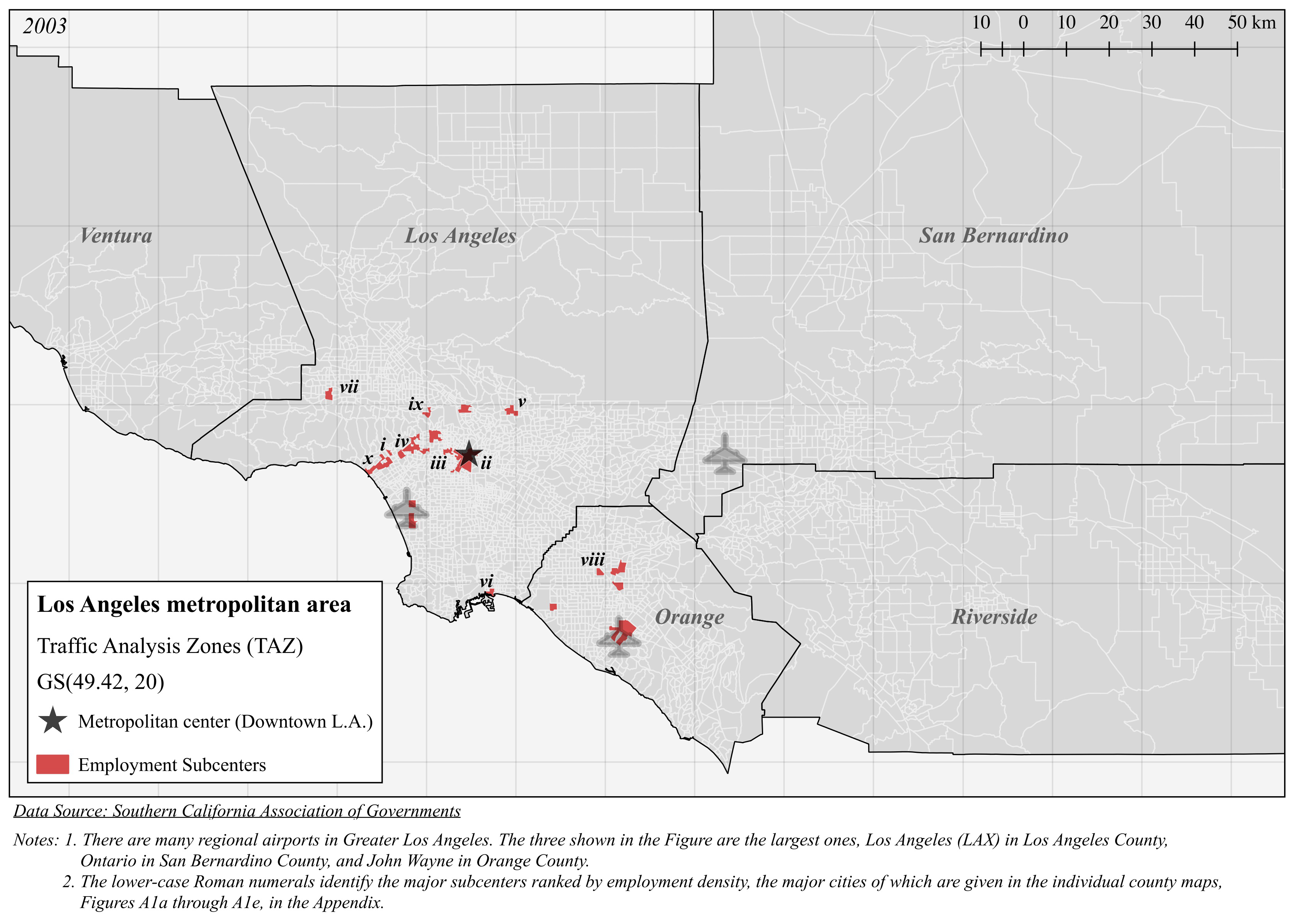
Figure 1. Los Angeles metropolitan area subcenters identified by GS(49.42, 20).
Land 06 00017 g001
Figure 2. Hypothetical metropolitan area subcenters identified by EDC(15, 15, l n 2 40 ).
Land 06 00017 g002
Figure 3. Los Angeles metropolitan area subcenters identified by EDC(49.42, 20; 0.01077).
Land 06 00017 g003
Figure 4. Los Angeles metropolitan area subcenters identified by: (a) DGC(49.42, 20, 1; 0.02173); (b) DGC(49.42, 20, 0.5; 0.02173).
Land 06 00017 g004
Figure 5. Calgary metropolitan area subcenters identified by: (a) DGC(49.42, 20, 0; 0.1139); (b) DGC(49.42, 20, 1; 0.1139); (c) DGC(49.42, 20, 0.5; 0.1139).
Land 06 00017 g005aLand 06 00017 g005b
Figure 6. Paris metropolitan area subcenters identified by: (a) DGC(49.42, 20, 0; 0.08041); (b) DGC(49.42, 20, 1; 0.08041); (c) DGC(49.42, 20, 0.5; 0.08041).
Land 06 00017 g006aLand 06 00017 g006b