Fire Data as Proxy for Anthropogenic Landscape Change in the Yucatán
by
Marco Millones
1,*, 
John Rogan
2, 
B.L. Turner II
3,
Benoit Parmentier
4,
Robert Clary Harris
5 and
Daniel A. Griffith
6 1
Department of Geography, University of Mary Washington, 1301 College Ave, Fredericksburg, VA 23219, USA
2
Graduate School of Geography, Clark University, 950 Main St. Worcester, MA 01610, USA
3
School of Geographical Sciences and Urban Planning, and School of Sustainability, Arizona State University, Tempe, AZ 88281-5302, USA
4
Sustainability Solutions Initiative, Mitchell Center, 5710 Norman Smith Hall, University of Maine, Orono, ME 04469, USA
5
Independent Scholar
6
School of Economic, Political and Policy Sciences, University of Texas at Dallas, 800 W Campbell Rd, Richardson, TX 75080, USA
*
Author to whom correspondence should be addressed.
Land 2017, 6(3), 61; https://doi.org/10.3390/land6030061
Submission received: 14 August 2017
/
Revised: 14 August 2017
/
Accepted: 8 September 2017
/
Published: 12 September 2017
(This article belongs to the Special Issue Anthropogenic Biomes)
Abstract
:Fire is one of the earliest and most common tools used by humans to modify the earth surface. Landscapes in the Yucatán Peninsula are composed of a mosaic of old growth subtropical forest, secondary vegetation, grasslands, and agricultural land that represent a well-documented example of anthropogenic intervention, much of which involves the use of fire. This research characterizes land use systems and land cover changes in the Yucatán during the 2000–2010 time period. We used an active fire remotely sensed data time series from the Moderate Resolution Imaging Spectroradiometer (MODIS), in combination with forest loss, and anthrome map sources to (1) establish the association between fire and land use change in the region; and (2) explore links between the spatial and temporal patterns of fire and specific types of land use practices, including within- and between-anthromes variability. A spatial multinomial logit model was constructed using fire, landscape configuration, and a set of commonly used control variables to estimate forest persistence, non-forest persistence, and change. Cross-tabulations and descriptive statistics were used to explore the relationships between fire occurrence, location, and timing with respect to the geography of land use. We also compared fire frequencies within and between anthrome groups using a negative binomial model and Tukey pairwise comparisons. Results show that fire data broadly reproduce the geography and timing of anthropogenic land change. Findings indicate that fire and landscape configuration is useful in explaining forest change and non-forest persistence, especially in fragmented (mosaicked) landscapes. Absence of fire occurrence is related usefully to the persistence of spatially continuous core areas of older growth forest. Fire has a positive relationship with forest to non-forest change and a negative relationship with forest persistence. Fire is also a good indicator to distinguish between anthrome groups (e.g., croplands and villages). Our study suggests that active fire data series are a reasonable proxy for anthropogenic land persistence/change in the context of the Yucatán and are useful to differentiate quantitatively and qualitatively between and within anthromes.
1. Introduction
This study examines anthropogenic land cover change and persistence across the Yucatán Peninsula of Mexico by incorporating fire occurrence as a geographic context-specific indicator of human land practices. Land use and land cover change (i.e., land change) is an International Council for Science (ICSU) millennial research challenge [1] and has been addressed by various research communities [2,3,4,5]. A consensus has emerged that human-induced land changes have increased at unprecedented rates throughout the last century [5,6,7] to such an extent that the long-term well-being of human-environment relationships now requires more sustainable management of land uses [8,9]. Without disagreeing with the previous assertion, other researchers have argued that humans have altered ecosystems to such a degree that present landscapes would be best characterized in terms of anthropogenic biomes or anthromes, as they occupy the largest portion of the terrestrial land surface [10]. These concerns have guided numerous efforts to detect, map, and monitor land change, especially with the aid of remote sensing technology (e.g., [11,12]). Complementary mapping efforts have been undertaken to understand the level of direct human influence, as well as efforts to model the causes, constraints, mechanisms, and trajectories of land change and persistence (e.g., [2,10,13,14,15,16]).
While much has been learned from these research efforts, certain research challenges remain unaddressed [4,16,17]. Two of these challenges are pertinent for highly dynamic and spatially heterogeneous mosaicked humanized landscapes: the need for additional explicit studies seeking to untangle region-specific human-environment interactions and the need to incorporate context and temporal information from satellite data sources into the analysis [4,16,17,18].
The accuracy and spatial explicitness of land use and land cover maps has improved in the past 20 years with the refinement of the spatial and spectral resolution of remotely sensed data [12,16,19]. For local-to-regional scale mapping, land change research has relied heavily on cross-sectional assessments (e.g., two or three map dates; [20]). Although valuable, cross-sectional approaches often overlook high frequency land dynamics occurring between land cover map dates [21] and can potentially misrepresent recurrent changes as unidirectional trends, leading to over- or under-estimation of change [22]. In the last decade, high temporal frequency remotely sensed datasets having1 km spatial resolution and improved calibration such as the Advanced Very High Resolution Radiometer (AVHRR), the Global Inventory Modeling and Mapping Studies (GIMMS) NDVI data and the MODIS data product suite [23] have been made available. While AVHRR and GIMMS data are ideal for monitoring dynamic, long-term environmental processes at continental and global scales [11,18,24,25], their application is limited at sub-national scales [20]. The MODIS product suite in contrast, although limited by its shorter time-span, offers not only better or equivalent spatial, spectral and temporal capacity [26], but also the potential use of the MODIS archive of derived products (e.g., sea ice, active fire) as ancillary data to yield improvements in land cover mapping and change detection (e.g., [27,28]).
In addition to improvements in spatial and temporal details of land cover mapping, researchers have made significant progress to specify and even re-conceptualize traditional land cover/land use categories. Specifically, the re-framing of categories in terms anthropogenic land use intensity (e.g., anthromes) places the focus on human activities. Many of these efforts have relied on population density to characterize differences between areas that are highly or sparsely intervened by humans. Heterogeneity is another criterion commonly used to characterize anthropogenic landscapes. In those instances, landscapes are often measured on a homogeneity continuum from highly heterogeneous areas of “built” landscapes combining many different land uses in relatively small areas, to others presenting large swaths of homogenous features [10].
Fire is one of the earliest and most significant tools used by humans to modify landscapes and to extract benefits from ecosystem goods and services (e.g., land clearing for agriculture or urban development, forest thinning). At the same time, human land use and management (e.g., fuel load quantity and distribution, regulation and ignition sources) have altered naturally occurring fire regimes [29,30,31]. The “pyric transition” model has been proposed to describe the relationship between human intervention and the intensity of fire use across time and space (e.g., none in dense urban contexts, high in agricultural extensive systems, low or background in relatively “untouched” ecosystems) [29]. This relationship, however, is highly context-specific, in terms of the biophysical and the cultural characteristics of a region.
The present study takes advantage of that potential by using MODIS active fire data time-series in combination with categorical land cover/use maps to examine the link between land change, human activities and fire in the Yucatán Peninsula.
2. Study Area
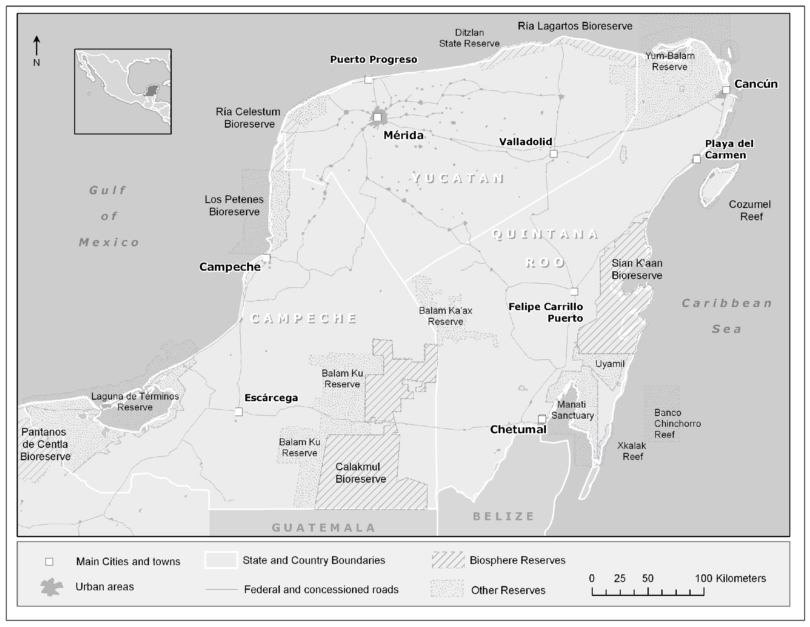
The Yucatán Peninsula (henceforth, the Yucatan), defined in this study by the Mexican states of Campeche, Quintana Roo and Yucatán (Figure 1), is a region characterized by a mostly flat, karstic, quaternary plain. The region is a highly dynamic and complex mosaic of subtropical dry forest in different states of ecological succession driven by human and environmental disturbance (e.g., fire, tropical storms, agriculture) [32,33,34,35]. Unless interrupted by specific disturbances such as fire-friendly plant invasion or management practices, post-fire vegetation grows back at a rapid rate after a burn. In much of the Yucatán Peninsula, secondary vegetation can reach a height of 10 m within-five years of clearing [36,37,38]. As a consequence, there is typically only a short window of time to detect land change.
Fire in the Yucatán is not only an environmental disturbance, but also the main land-clearing tool in the region. It precedes most land conversion (e.g., urbanization, clear-cut deforestation) and land modification events such as shifting cultivation, pasture maintenance, and secondary vegetation regrowth [32,37,38,39,40]. Persistence and maintenance of non-forest land cover types (e.g., pasture, various crops, early secondary vegetation) are also controlled by fire. In the Yucatán, two types of fire are commonly distinguished by local population and regulation: quemas and incendios. Quemas (~agricultural burns) are, in theory, legally registered and strictly regulated and scheduled for the purpose of swidden (slash-and-burn) agriculture. This includes subsistence maize-based cropping (milpa), pasture maintenance and mechanized agriculture (e.g., sugar cane, commercial corn). Incendios forestales (wildfires) are, in theory, accidental fires that are ignited by cigarette butts, broken glass, or lightning. They typically occur during the dry season (March–May), can affect large areas and last for several days. These fires, if a consequence of human action, are illegal and usually generate government agency response, especially if they grow out of control and affect farming, forest extraction and natural protected areas (NPA) [40,41]. Although the distinction can be easily blurred (e.g., escaped burns), quemas tend to be more ubiquitous in the region, are smaller in area, and shorter in duration than incendios. In contrast, incendios are less frequent, cover large areas, and temporally discrete events that are often amplified in contact with hurricane blow downs [42].
Given the previously described links between various human activities and fire practices, we expect that the spatio-temporal pattern of fire can serve as a proxy for certain anthropogenic land use practices in the Yucatán (e.g., milpa, mechanized agriculture, sugar cane cultivation and new urban development). Naturally occurring wild fires are less frequent in this region than fire of anthropogenic origin. This characteristic represents an opportunity to evaluate fire as a proxy for various land uses and land cover changes in the region.
The primary goal of this study is to assess land cover change and persistence across the Yucatán Peninsula by incorporating MODIS active fire occurrence data as a site-specific indicator of human-induced land change. The specific objectives are to: (a) describe the spatio-temporal dynamics of fire and its association with land use practices and land change; (b) determine the importance of fire presence to explain types of land persistence and change using a spatial multinomial logit model; and, (c) explore the ability of fire frequency to discriminate between anthropogenic landscape types (anthropogenic biomes or anthromes).
Beside the specific goal stated, lessons learned in this study may be of wider interest in other regions of the world. Spatial driver variables used for land-change modeling and prediction are typically expensive to produce or not frequently updated as most countries and regions do not possess such information at the level of detail required. Similarly, land cover maps are rarely produced annually. Most land cover maps are commonly produced using a census like approach with 5–10 years gaps at the country or regional levels. For an increasing number of applications, mapping rapid changes within-these temporal gaps across countries boundaries may be crucial. It is in this context that active fire data becomes useful as a predictor. It has both high temporal frequency and is readily available worldwide. To evaluate the usefulness of fire as predictor in both data poor and rich areas, we modeled land change with and without the presence of additional spatial drivers. Results reported in this specific study should therefore be of potential interest to a wider audience of researchers and land management practitioners.
3. Methodological Approach
3.1. Data
A comprehensive active fire dataset was constructed using NASA’s 1 km MOD14A2 (from TERRA) and MYD14A2 (from AQUA) 8-day composite product, using various time ranges within-the time period 2000–2010 [43] in order to match fire data and land cover data availability. Both data products provide detection confidence levels [44] of which only high and medium were used in order to minimize potential false positive detections [27,45] (Figure 2). The 1 km fire grid cell locations were converted to centroid points to match and extract the 30 m grid cell land cover attributes [42].
Land change/persistence information was obtained from Southern Mexico Forest Cover and Clearance from c. 1990 to c. 2000 and to c. 2007 digital maps developed by the Center for Applied Biodiversity Science (CABS) at Conservation International [46]. The original maps are based on the interpretation of (~30 m resolution) Landsat-5 Thematic Mapper satellite imagery, and are composed of five categories: forest, non-forest, mangrove, water, and cloud/shadow. Forest cover is defined as mature forest >3 m closed canopy [44]. Thematic map accuracy was reported to have a Kappa index of 86% with an error of commission of 11.27% and an error of omission of 4.86% for the dominant tropical dry forest class prevalent in the study area [44]. Forest and mangrove classes were merged, whereas water, clouds and shadow pixels were masked and removed from further analysis to produce a map of land persistence and change for 2000–2007, with three resulting categories: forest persistence (FP), non-forest persistence (NFP), and forest-to-non-forest (CH) (Figure 3). It must be noted that in contrast with FP (“old growth” forest persistence), NFP by definition, allows for land changes between sub-classes within-a broad non-forest category. For example, a transition from agriculture to pasture or from pasture to secondary forests would be included in NFP. Although lacking detailed land categories, the resulting three-category map has the advantage of being more consistent than most multi-temporal assessments because it was produced using a consistent methodology by the same research team explicitly for the purpose of forest change mapping [46,47].
Anthrome map data corresponding to time interval 2001–2006 were obtained from the SEDAC website [48]) in GeoTIFF format. We cropped and match the dataset to the Yucatán region and aggregated the original 21 anthrome categories using the six anthrome group classification: Dense settlements, villages, croplands, rangelands, forested, wildlands. In order to match the temporal and spatial resolutions, an additional fire variable was created from the MODIS time series by aggregating years (2001–2008), matching projection and, coarsening the cell size. This resulted in a 10 × 10 km fire frequency map used for the anthrome analysis.
Additional variables commonly used in land-change modeling were included in the analysis to control for environmental and socio-economic factors. Elevation and slope were derived from a 90 m SRTM digital elevation model. Precipitation data were derived from Tropical Rainfall Measuring Mission (TRMM). Protected Areas from CONANP (Mexican Natural Protected Area Commission) were processed to match the study area. Communal property lands (ejidos), population density change, as well as the distance to road variable were derived from the Mexican Census Bureau [49]. Cattle density by municipality was obtained from the 2007 Censo Agropecuario [49].
Even though MODIS fire data are constantly updated, in this study, we only include data to the year 2010. We consider the 2000–2010 ten-year period sufficient to describe the salient points about the spatio-temporal patterns of a fire in the region. More importantly, the land cover data and anthrome data that we use do not go beyond 2007 and 2008, respectively. For this same reason, the multinomial modeling component of this study does not use any fire data from after 2007 (see methods section).
3.2. Methods
The methodology has three components: (a) a characterization of the spatio-temporal patterns and co-location of land change/persistence and fire; (b) an assessment of the effect of fire presence, landscape patch size and other covariates land-change outcomes (FP, NFP and CH), using a spatial multinomial logit model for the period 2000–2007; and, (c) an exploration of the ability of fire frequency to distinguish human landscape categories defined in anthrome groups and anthrome classes.
3.3. Characterization of Land Change and Fire Patterns
A cross-tabulation-based change analysis was performed on the simplified CABS land cover map pairs 1990–2000 and 2000–2007, resulting in one map with two persistence classes (FP and NFP) and one change class (CH) (Figure 3). Spatio-temporal dynamics of fire occurrence were derived by manipulating the MODIS fire archive via map algebra operations (e.g., overlay, reclassification) into map and graph summaries of annual and multi-year fire frequency. After accounting for the different time-spans of the TERRA and AQUA series and adjusting for double counting, three separate fire occurrence sets were created: a TERRA ten-year summary map (2000–2010) (Figure 2) and a TERRA-AQUA combined annual time-series graph (2000–2009) (Figure 4). Global (Moran’I) and local (Getis-Ord Gi* and LISA) measures of spatial autocorrelation were calculated for all sets of maps [50,51,52]. Finally, a second cross-tabulation analysis was performed for the land change/persistence map (FP, NFP and CH) (Figure 3) and the binary fire (reclassification of Figure 2) maps in order to describe and explore the spatial correspondence between them and the relationship between fire occurrence and the different land cover categories. The result of this cross-tabulation map is shown in Figure 5.
3.4. Effect of Fire and Patch Size on Land Change/Persistence: A Spatial Multinomial Logit Model
A spatial multinomial logit model using 2003–2007 fire “density” or “intensity” (fire count/five years) as independent variable (FIRE), and 7 control variables was performed. This model specification is used in the literature (e.g., [53,54]) and is preferred because the dependent variable consists of three possible outcomes that are categorical/nominal in nature [55,56,57]. To account for the positive spatial autocorrelation present in remotely sensed data [58,59] spatial lags variables based on rook-case adjacency were calculated. This was done by generating, for each observation, the average sum of its neighbors of the same class (CFP, CNFP, and CCH), and including the lag variable in the model (see Equation (1)) [59,60]. Lag values range from 0 (no like neighbors) to 1 (all four like neighbors), while average Moran’s I values range from virtually random for CCH (0.0035) to weak-moderate positive for CNFP (0.392) and CFP (0.391). In this particular case, spatial lags also serve as an indicator of landscape configuration and heterogeneity (i.e., similar to patch size and cohesion).
Pseudo-likelihood estimates were calculated for the main effects and spatial lag parameters of the multinomial model as follows (Equation (1)):
where πhij is the probability that a pixel h in the map of any class i for which fire has been detected will become one of land change/persistence category j (FP, NFP or CH), j ≠ r, with land change/persistence category r being the reference category. There are separate sets of intercept parameters αj and regression parameters βj for each of the logit models. The matrix x′hi is the set of explanatory variables: spatial lag (CY), fire (FIRE), and the commonly used control variables described. Two logits equations are modeled for each FIRE and CY population: the logit comparing non-forest persistence (NFP) to forest persistence (FP) and the logit comparing change (CH) to forest persistence (FP) [56].
Log(πhij/πhir) = αj + x′hi βj
3.5. Fire Frequency and Anthromes Characterization
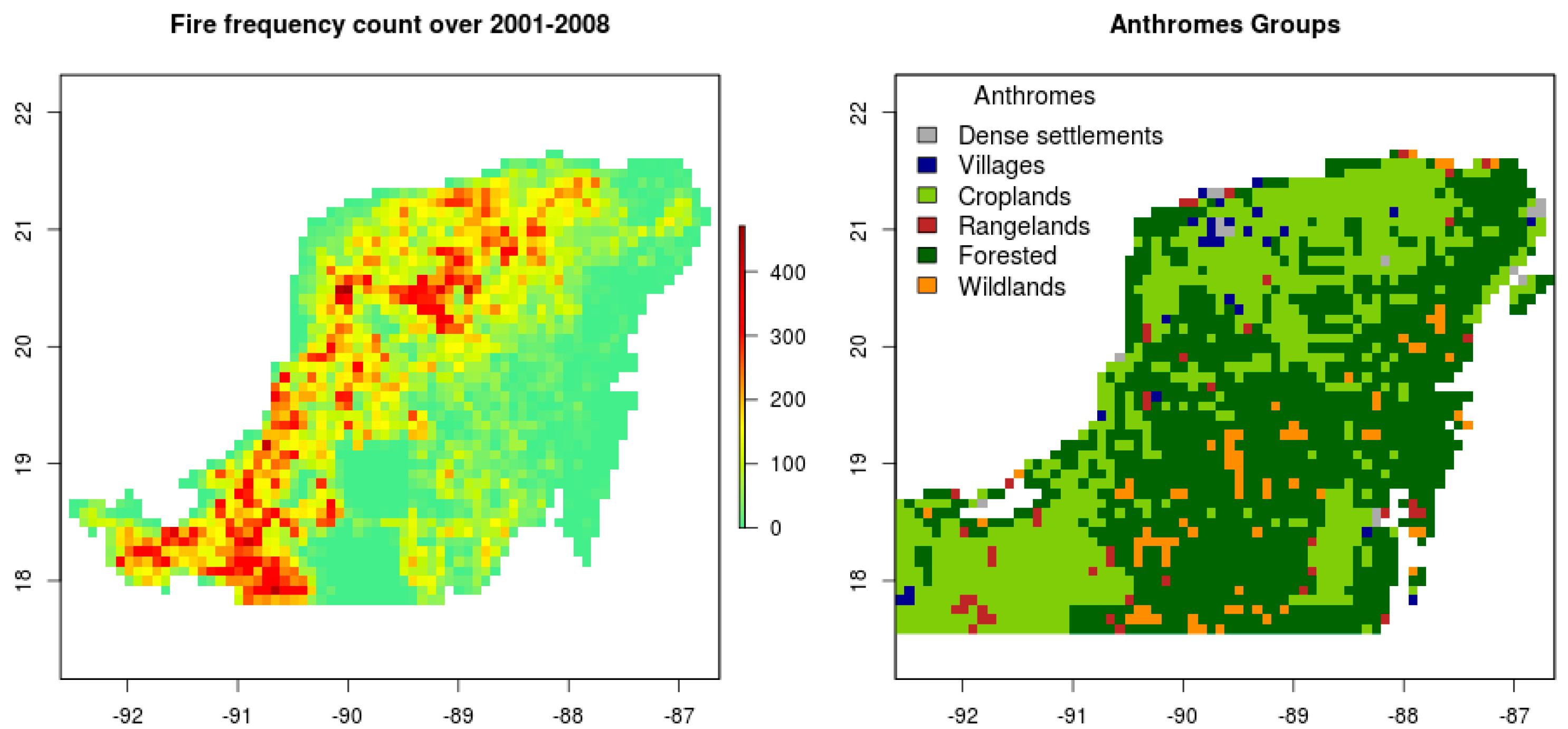
Anthromes map datasets were processed to match them to the study area, and temporal fire count data were aggregated to generate a fire frequency variable (Figure 6). In order to explore the association between fire counts and anthrome groups graphically, we used boxplots of mean fire frequency by each category present in the study area: dense settlements, villages (in effect, village and surrounding areas), croplands, rangelands, forested, wildlands. We measured the differences in mean fire frequency across anthromes using a negative binomial model and a Tukey pairwise comparison. A binomial model was preferred over Poisson model because the overall (as well as per category) mean and variance are noticeably different (by a factor 100), which suggests over-dispersion in the Poisson parameter. We also conducted Tukey comparisons for fire frequency within the cropland anthromes group to assess the potential of using fire count for finer definition of the human imprint of landscape.
For the data processing, we used the raster (version 2.5-8), sp (version 1.2-4) and rgdal (version 1.2-7) packages to perform some of the preprocessing for the spatial inputs. The raster package was also used for aggregation of the fire occurrences, cropping and reclassification of anthromes data. We used the implementation of multinomial model in the R “nnet” package (version 7.3-12) for analyses. We also ran the negative binomial model using the “MASS” package (version 7.3-12) in R version 3.4 and used the glht method from the multcomp R package (1.4-6) to perform the Tukey comparison.
4. Results
4.1. Spatio-Temporal Patterns of Fire and Land Change
As a proxy indicator of human land use, fire frequency can be interpreted as a quantitative measure of “density” (in space and time) of land use in this case. It corresponds to how actively “used” or “under-used” a 1 km parcel of land is in relation to the types of land use that require burning (e.g., high for pasture and cultivation land).
Fire occurrence for the period 2000–2010 presents a distinct non-random spatial pattern across the study area (Moran’s I = 0.62) (Figure 2). The individual observations presenting the highest detection frequencies (>3 per year) appear in spatial clusters and are concentrated in the northern and western section of the Peninsula in the states of Campeche and the Yucatán. Quintana Roo has comparatively fewer and less clustering fire detections. Areas with less fire frequency are observed in Campeche and Quintana Roo, especially in the presence of federal and state run natural protected areas (e.g., Sian Ka’an and Calakmul bioreserves) (Figure 1), and in locations where road and settlement density is low. This road-settlement-fire co-location is more explicit in the Yucatán and northern Campeche, and less so in southern Campeche, where road density decreases.
Locations affected by fire (Figure 5 and Table 1) cover roughly 45% of the study area. More than half of the fire occurrences concentrate in NFP areas, followed by 40% of FP, and 2% in CH areas (1% of the total). Locations with no fire occurrence cover more than 50% of the study area. No-fire occurrences are two times more common in FP than in NFP, and they are minimally present in CH areas. Land change/persistence figures (total rows percentage in Table 1) indicate that roughly 2/3 of the FP shows no fire detections, whereas 60% of NFP presents fire occurrence. CH shows 86% of its area as having burned at some time (although it is hardly visible in Figure 5, because CH covers only 1% of the total area).
4.2. Effect of Fire and Patch Size on Land Change/Persistence: A Spatial Multinomial Logit Model
Results from the spatial multinomial logit model agree with the analysis presented above (Section 4.1) and indicate that past fire occurrence (pre-2007) is a useful predictor of land change/persistence categories. The resulting equations and model statistics are summarized in Table 2 and in the supplementary Appendix A. The Akaike information criterion (AIC) indicates that the model with covariates (intercept + fire and lag + control variables) performs better than alternative models (see Appendix A). The likelihood ratio (LR) has two degrees of freedom and is significant, which confirms that at least one of the variables in the model improves the model description.
The maximum pseudo-likelihood and odds ratio point estimates (Table 2 and Appendix A) show the effect and relative importance of FIRE and CY for each land change/persistence outcome in the model. At a 5% level, the difference between FIRE = 1 (fire occurrence) and FIRE = 0 is statistically different for all cases (FP, NFP and CH), for all three states separately and the three-state aggregated study area. CY is a significant covariate in the model for all of these cases. Additional models were run with control variables. These full model results are presented in the Appendix A and confirm the usefulness of fire as predictor.
An inspection of the pseudo-likelihood estimates for the aggregated study area (Table 2 and Appendix A) indicates that for each unit increase in FIRE (intensity), the log of the ratio of p(CH)/p(FP) increases by ~1.92, and the log of the ratio of p(CH)/p(NFP) increases by ~0.2. In other words, for each unit increase in FIRE (intensity) in a given pixel (in Figure 2), the odds of that same pixel belonging to category CH (forest to non-forest change) rather than category FP (forest persistence in Figure 3) are multiplied by ~6.7. Unit increases in FIRE also increase the odds of a pixel belonging to category CH rather than NFP (no forest persistence) by 1.22.
For every increase in one unit of Fire, the odds of a pixel belonging to category NFP instead of CH are multiplied by 0.82. For every increase in one unit of Fire, the odds of a pixel belonging to category NFP instead of FP are multiplied by 5.59. For every increase in one unit of Fire, the odds of a pixel belonging to category FP instead of CH are multiplied by 0.15 (almost none).
For every increase in one unit of Fire, the odds of a pixel belonging to category FP instead of NFP are multiplied by 0.18 (almost none). Overall FIRE estimates are negative when predicting forest persistence (FP) and positive when predicting CH.
The calculated spatial lag (CY) terms are significant for all cases. CY, as mentioned earlier, can be interpreted as cohesiveness of land cover patches [61]. Larger CY values correspond to more similar values among neighboring cells (i.e., a larger patches of a category). Estimates of the model for the aggregated peninsula indicate that a unit increase in CY decreases the log of p(FP)/p(CH) by ~−3.55, while the log of p(FP)/p(NFP) decreases by ~−0.07. This finding indicates that persistent forest areas located in large patches are very likely to remain forest (34 times more than CH) (Table 2 and Appendix A). FP is also 1.07 times more likely than NFP. In general, CH has a negative relationship with CY. This relationship can be attributed to CH occurring more often in isolated pixels corresponding to fragmented patches. Conversely, FP and NFP occur in larger continuous areas (Figure 3).
4.3. Comparison of Fire by Anthromes
Boxplots of mean fire frequency by anthromes groups suggest that fire can be used to distinguish among anthromes groups thereby serving as an additional potential variable to examine human imprints in the context of the Yucatán region (Figure 6). The croplands anthromes group has a higher fire frequency on average compared to most other anthromes categories. We note that rangelands display a very large variance and thus may be difficult to distinguish from croplands and villages. Finer anthropogenic categories within the cropland groups also appear to be contrasted by the fire frequency variable (see boxplots Figure 7).
Tukey pairwise comparison tests between anthromes groups (applied to the negative binomial model Table 3) highlight that six and seven pairwise comparisons are significantly different at 5% and 10% level respectively. Coefficients indicate relative increase or decrease of the expected log of fire frequency for categorical change in relation to the reference variable. For instance, there is a −1.37 decrease in the log of fire frequency when an observation is found in the dense settlements rather than in croplands. We find that fire frequency variable is useful to differentiate croplands with almost all categories with the exception of Villages and Rangelands. Both overlap substantially on the boxplots (Figure 7).
Tukey comparisons were also performed for fire frequency within the cropland anthromes group to assess the potential of using fire frequency for finer definition of the human imprint of landscape. We found that within croplands two out 10 and four out of 10 comparison results in significant differences in the log of fire frequency (Table 4) at 5 and 10 percent significance level, respectively. This suggests that fire frequency is less useful at distinguishing within the cropland anthromes. The strongest contrasts are found between “residential rainfed mosaics–remote croplands mosaic” and between “residential irrigated cropland–remote croplands”. Both indicate decreases in the log of fire frequency for locations that are found in residential rainfed and irrigated cropland compared to remote croplands.
5. Discussion and Conclusions
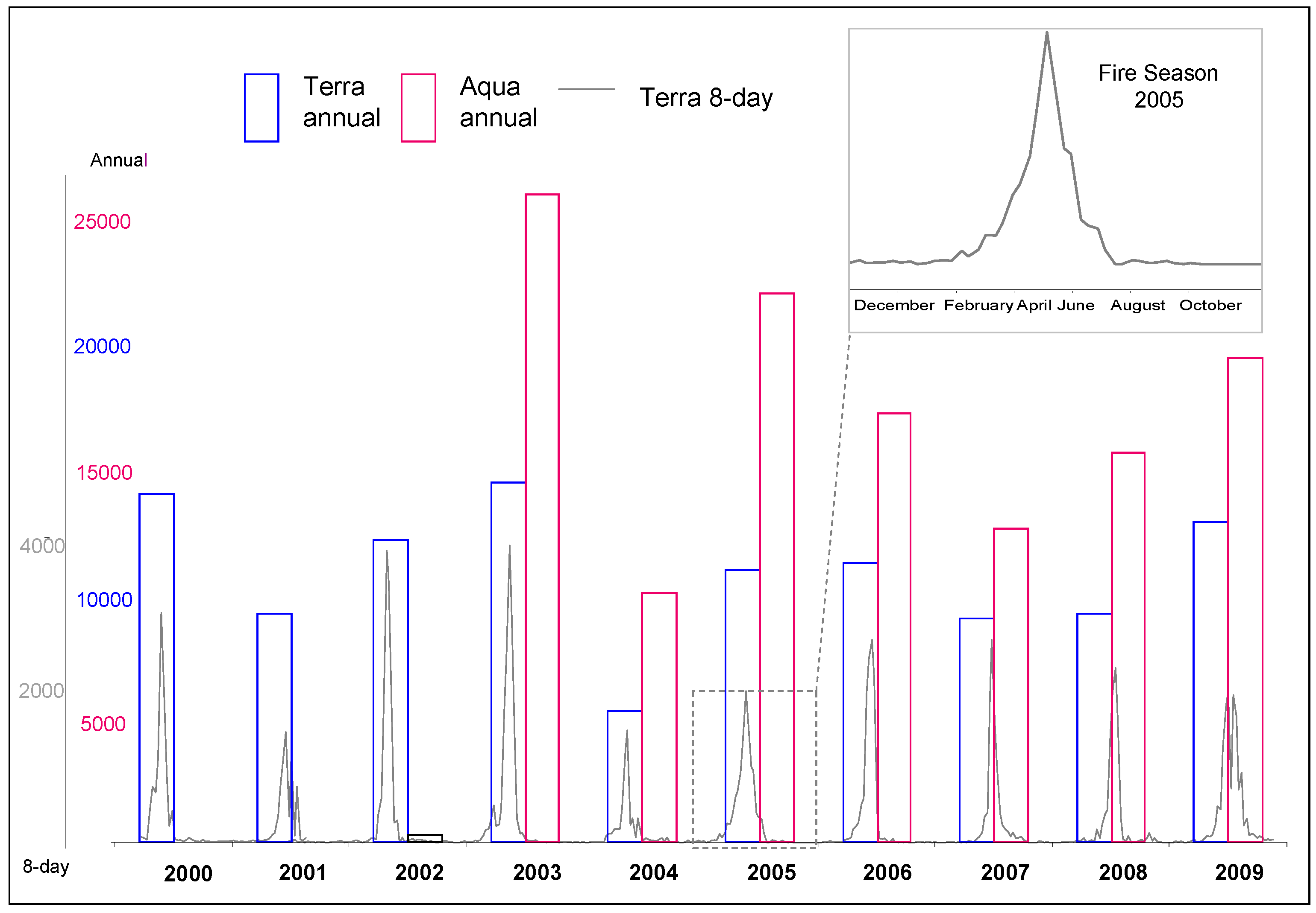
Analysis of the spatial patterns of fire in the Yucatán using fire data visually reproduces the geography of human land-based activities during 2000–2010, including the influence of roads, settlements, and natural protected areas. The intra-annual temporal dimensions of fire data approximate key moments of seasonal agriculture and other land-based activities (Figure 4). These findings are consistent with studies finding higher fire frequencies in the proximity to roads and settlements region [40], and with research about fire and deforestation in other tropical settings (e.g., [28,62,63,64]) and more generally, about the relationship between land change, road development and market accessibility [53,54,64,65].
The multinomial model confirms the significance of fire intensity (defined as count of fire flagged pixels over time) and landscape configuration (represented by the spatial lag variable CY) for the peninsula for all three types of land change/persistence outcomes. Notably all change is strongly affected by the presence of fire. The odds of a forested area becoming non-forested multiply by six in the presence of fire. This is not surprising given that the cross-tabulation analysis showed that nearly 87% of pixels that changed from 2000 to 2007 had been flagged as fire by MODIS at some point. The dominance of no-fire observations over fire occurrence, the (pseudo) absence of fire, makes for a better predictor of forest persistence than fire occurrence per se, especially for large patches (high CY values). Predicting non-forest persistence proved more difficult, signaling the diversity of ecological and land use practices and transitions between them that define the NFP category as discussed in the data section. What exactly accounts for the remaining 13% is difficult to determine. We can speculate however that possible factors include data error and accuracy mismatches. As some have noted, MODIS products do omit fires for various reasons [40]. We can also speculate on some detected fires being non-agricultural. Finally, we can also imagine some fires starting as agricultural burns but becoming large multiday forest fires as they grow out of control [40].
Fire also proves to be a reasonable indicator to distinguish between anthromes groups (Figure 7) but less among finer anthromes categories. Our analysis shows that, for example, with the aid of a fire frequency croplands are separable from the rest of categories and that dense settlements are clearly distinct from villages. Other categories like rangeland prove more difficult to separate since they present larger variance. Some within-variation within anthropogenic categories is also distinguishable. For example, populated irrigated is clearly separable from populated rainfed and from remote croplands. These two former categories, however are not as separable from each other with the aid of fire frequency alone.
Perhaps some insight about differences distinguishing between- and within-anthropogenic landscapes can be gained by looking into the distinction between quemas (legally regulated agricultural fires) from incendios (large escape non-regulated forest fires). Both can be addressed through the use of MODIS active fire data, but cannot be thoroughly distinguished with these data alone. Within-variation exists in both categories. On the one hand, quemas can be due to subsistence and commercial agriculture, such as sugar cane cultivation along the border with Belize (i.e., either rain fed or irrigated anthrome categories), or Mennonite corn fields in Bacalar,( i.e., the populated irrigated anthrome category), as their spatial and temporal signatures can differ quite noticeably (Figure 2 and Figure 4). On the other hand, incendios can be truly accidental or be the result of purposeful burning with nonagricultural goals (e.g., forcing land zoning code changes for urban development, hunting practices). Future research should exploit these differences in order to account for a more nuanced description of the relationships between fire and human-induced land change in the region.
We conclude that in subtropical forest settings, in which burning is a fundamental landscape tool, fire is a reasonable proxy for land change. Use of fire data improves the estimation of land change and expands our understanding of human-environment relationships that produce complex mosaics of highly dynamic landscapes, such as those in the Mexican Yucatán.
Acknowledgments
This study was part of the SYPR (http://sypr.asu.edu) and EDGY (http://landchange.rutgers.edu) projects. SYPR received support from the NASA LCLUC program (NAG-56046, 511134 and 6GD98G) and the NSF BCS program (0410016). EDGY was sponsored by the Gordon and Betty Moore Foundation under Grant #1697. The authors thank Drs. Birgit Schmook (El Colegio de la Frontera Sur), Laura Schneider (Rutgers University) and Zachary Christman (Rowan University) for their support and advice. The staff of Clark Labs facilitated the work by creating and maintaining the Idrisi® software (http://www.clarklabs.org/) with which preliminary analysis was performed. Subsequent and final analysis was performed with R packages: NNet, MASS, multcomp, and raster.
Author Contributions
Marco Millones, John Rogan, B.L. Turner II conceived and designed the original research and fieldwork; Marco Millones performed the fieldwork; Marco Millones performed preliminary data analysis with Daniel A. Griffith, Robert Clay Harris and Benoit Parmentier executed the final data analysis; John Rogan, B.L. Turner II revised earlier versions of the manuscript; Marco Millones, Benoit Parmentier and Robert Clay Harris wrote the paper. John Rogan revised the manuscript.
Conflicts of Interest
The authors declare no conflicts of interest.
Appendix A

Table A1.
Multinomial Logistic Model Results (variable definitions below).
| LN[p(NFP)/(FP)] | |||||
| Estimate | Odds | p-Value | Standard Error | z-Score | |
| Intercept | 4.38 | 79.63 | 0.00 | 0.00 | 30,014.70 |
| CY | −0.07 | 0.94 | 0.00 | 0.00 | −537.22 |
| fire density | 1.72 | 5.59 | 0.00 | 0.00 | 66,617.78 |
| distance to roads | −0.54 | 0.58 | 0.00 | 0.00 | −428.23 |
| Elevation | −0.01 | 0.99 | 0.00 | 0.00 | −74.17 |
| slope (degrees) | −0.06 | 0.95 | 0.00 | 0.00 | −15.75 |
| cattle density | 0.06 | 1.06 | 0.00 | 0.00 | 58.25 |
| ejido lands | −0.39 | 0.68 | 0.00 | 0.00 | −4265.32 |
| population density change | 0.00 | 1.00 | 0.87 | 0.00 | 0.17 |
| precipitation | 0.00 | 1.00 | 0.00 | 0.00 | −7.67 |
| protected areas | 0.46 | 1.59 | 0.00 | 0.00 | 7034.54 |
| Soil | −0.10 | 0.91 | 0.00 | 0.00 | −4248.04 |
| LN[p(FP)/(NFP)] | |||||
| Estimate | Odds | p-Value | Standard Error | z-Score | |
| Intercept | −4.38 | 0.01 | 0.00 | 0.00 | −29,981.84 |
| CY | 0.07 | 1.07 | 0.00 | 0.00 | 530.89 |
| FIRE_intensity | −1.72 | 0.18 | 0.00 | 0.00 | −67,202.89 |
| dist_roads | 0.54 | 1.72 | 0.00 | 0.00 | 427.89 |
| Elevation | 0.01 | 1.01 | 0.00 | 0.00 | 74.14 |
| slope_deg | 0.06 | 1.06 | 0.00 | 0.00 | 15.74 |
| cattledensity | −0.06 | 0.94 | 0.00 | 0.00 | −58.13 |
| ejido | 0.38 | 1.47 | 0.00 | 0.00 | 4261.07 |
| popdens_chenge | 0.00 | 1.00 | 0.71 | 0.00 | −0.37 |
| precip | 0.00 | 1.00 | 0.00 | 0.00 | 7.65 |
| protegidas | −0.46 | 0.63 | 0.00 | 0.00 | −7048.05 |
| soil | 0.10 | 1.10 | 0.00 | 0.00 | 4244.83 |
| LN[p(NFP)/(CH)] | |||||
| Estimate | Odds | p-Value | Standard Error | z-Score | |
| Intercept | 9.05 | 8498.41 | 0.00 | 0.00 | 123,593.53 |
| CY | 3.48 | 32.43 | 0.00 | 0.00 | 55,698.76 |
| FIRE_intensity | −0.20 | 0.82 | 0.00 | 0.00 | −14,938.93 |
| dist_roads | −0.43 | 0.65 | 0.00 | 0.00 | −687.67 |
| elevation | 0.00 | 1.00 | 0.03 | 0.00 | −2.15 |
| slope_deg | 0.58 | 1.79 | 0.00 | 0.00 | 327.37 |
| cattledensity | 0.11 | 1.11 | 0.00 | 0.00 | 218.22 |
| ejido | −0.25 | 0.78 | 0.00 | 0.00 | −5330.41 |
| popdens_chenge | −0.06 | 0.95 | 0.00 | 0.00 | −45.86 |
| precip | 0.00 | 1.00 | 0.00 | 0.00 | −39.16 |
| protegidas | 1.65 | 5.19 | 0.00 | 0.00 | 50,114.19 |
| soil | 0.42 | 1.52 | 0.00 | 0.00 | 35,985.19 |
| LN[p(CH)/(FP)] | |||||
| Estimate | Odds | p-Value | Standard Error | z-Score | |
| Intercept | −4.67 | 0.01 | 0.00 | 0.00 | −1,052,724.45 |
| CY | −3.55 | 0.03 | 0.00 | 0.00 | −770,643.97 |
| fire density | 1.92 | 6.79 | 0.00 | 0.00 | 1,416,356.73 |
| distance to roads | −0.11 | 0.90 | 0.00 | 0.00 | −4430.60 |
| elevation | −0.01 | 0.99 | 0.00 | 0.00 | −3.57 |
| slope (degrees) | −0.64 | 0.53 | 0.00 | 0.00 | −66,666.61 |
| cattle density | −0.05 | 0.95 | 0.00 | 0.00 | −1931.87 |
| ejido lands | −0.14 | 0.87 | 0.00 | 0.00 | −16,873.16 |
| population density chanve | 0.06 | 1.06 | 0.00 | 0.00 | 44.88 |
| precipitation | 0.00 | 1.00 | 0.00 | 0.00 | 39.04 |
| protected areas | −1.18 | 0.31 | 0.00 | 0.00 | −1,358,343.49 |
| soil | −0.52 | 0.59 | 0.00 | 0.00 | −423,156.99 |
| LN[p(CH)/(NFP)] | |||||
| Estimate | Odds | p-Value | Standard Error | z-Score | |
| Intercept | −6.07 | 0.00 | 0.00 | 0.00 | −1,974,081.65 |
| CY | −3.46 | 0.03 | 0.00 | 0.00 | −851,530.90 |
| FIRE_intensity | 0.20 | 1.22 | 0.00 | 0.00 | 215,160.66 |
| dist_roads | 0.44 | 1.55 | 0.00 | 0.00 | 34,899.45 |
| elevation | 0.00 | 1.00 | 0.03 | 0.00 | 2.15 |
| slope_deg | −0.47 | 0.62 | 0.00 | 0.00 | −46,646.59 |
| cattledensity | −0.11 | 0.89 | 0.00 | 0.00 | −2457.85 |
| ejido | 0.24 | 1.28 | 0.00 | 0.00 | 51,274.32 |
| popdens_chenge | 0.05 | 1.05 | 0.00 | 0.00 | 41.32 |
| precip | 0.00 | 1.00 | 0.03 | 0.00 | 2.21 |
| protegidas | −1.59 | 0.20 | 0.00 | 0.00 | −2,424,094.75 |
| soil | −0.47 | 0.62 | 0.00 | 0.00 | −526,363.39 |
| LN[p(FP)/(CH)] | |||||
| Estimate | Odds | p-Value | Standard Error | z-Score | |
| Intercept | 4.67 | 106.73 | 0.00 | 0.00 | 63,882.24 |
| CY | 3.55 | 34.66 | 0.00 | 0.00 | 56,986.69 |
| FIRE_intensity | −1.92 | 0.15 | 0.00 | 0.00 | −148,047.18 |
| dist_roads | 0.11 | 1.11 | 0.00 | 0.00 | 167.04 |
| elevation | 0.01 | 1.01 | 0.00 | 0.00 | 3.57 |
| slope_deg | 0.64 | 1.90 | 0.00 | 0.00 | 358.84 |
| cattledensity | 0.05 | 1.05 | 0.00 | 0.00 | 102.76 |
| ejido | 0.14 | 1.15 | 0.00 | 0.00 | 3038.12 |
| popdens_chenge | −0.06 | 0.95 | 0.00 | 0.00 | −44.85 |
| precip | 0.00 | 1.00 | 0.00 | 0.00 | −39.10 |
| protegidas | 1.18 | 3.27 | 0.00 | 0.00 | 35,911.95 |
| soil | 0.52 | 1.68 | 0.00 | 0.00 | 44,599.37 |
Intercept, CY = spatial lag; FIRE_intensity = fire flagged pixel count divided by five years; dist_roads = distance to roads; elevation = SRTM DEM derived elevation; slope_deg = DEM derived slope; cattle density = cattle density; ejido = communal land property status (binary); popdens_change = population density change; precipitation = precipitation derived from TRMM; protegidas = natural protected areas (binary); soil = binary soil.
References
- Reid, W.V.; Chen, D.; Goldfarb, L.; Hackmann, H.; Lee, Y.T.; Mokhele, K.; Ostrom, E.; Raivio, K.; Rockström, J.; Schellnhuber, H.J.; et al. Earth System Science for Global Sustainability: Grand challenges. Science 2010, 330, 916–917. [Google Scholar] [CrossRef] [PubMed]
- Irwin, E.G.; Geoghegan, J. Theory, data, methods: Developing spatially explicit economic models of land use change. Agric. Ecosyst. Environ. 2001, 85, 7–24. [Google Scholar] [CrossRef]
- Agarwal, C.; Green, G.M.; Grove, J.M.; Evans, T.P.; Schweik, C.M. A Review and Assessment of Land-Use Change Models: Dynamics of Space, Time and Human Choice; Technical Report NE-297; United States Department of Agriculture (USDA): Burlington, VT, USA, 2002.
- Turner, B.L.; Lambin, E.F.; Reenberg, A. The Emergence of Land Change Science for Global Environmental Change and Sustainability. Proc. Natl. Acad. Sci. USA 2007, 104, 20666–20671. [Google Scholar] [CrossRef] [PubMed]
- Griggs, D.; Stafford-Smith, M.; Gaffney, O.; Rockström, J.; Öhman, M.C.; Shyamsundar, P.; Steffen, W.; Glaser, G.; Kanie, N.; Noble, I. Policy: Sustainable development goals for people and planet. Nature 2013, 495, 305–307. [Google Scholar] [CrossRef] [PubMed]
- Steffen, W.; Sanderson, R.A.; Tyson, P.D.; Jäger, J.; Matson, P.A.; Moore, B., III; Oldfield, F.; Richardson, K.; Schellnhuber, H.J.; Turner, B.L.; et al. Global Change and the Earth System: A Planet under Pressure; Springer: Berlin/Heidelberg, Germany; New York, NY, USA, 2004. [Google Scholar]
- Foley, J.A.; DeFries, R.; Asner, G.P.; Barford, C.; Bonan, G.; Carpenter, S.R.; Chapin, F.S.; Coe, M.T.; Daily, G.C.; Gibbs, H.K. Global consequences of Land Use. Science 2005, 309, 570–574. [Google Scholar] [CrossRef] [PubMed]
- Turner, B.L., II; Skole, D.; Sanderson, S.; Fischer, G.; Fresco, L.; Leemans, R. Land-Use and Land-Cover Change Science/Research Plan; IGBP Report No. 35; The International Geosphere-Biosphere Programme IGBP: Stockholm, Sweden, 1995. [Google Scholar]
- Kates, R.W.; Clark, W.; Corell, R. Sustainability Science; KSG Working Paper No. 00-018; John F Kennedy School of Government (KSG), Harvard University: Cambridge, MA, USA, 2000.
- Ellis, E.C.; Ramankutty, N. Putting people in the map: Anthropogenic biomes of the world. Front. Ecol. Environ. 2008, 6, 439–447. [Google Scholar] [CrossRef]
- Loveland, T.R.; Sohl, T.L.; Stehman, S.V.; Gallant, A.L.; Sayler, K.L.; Napton, D.E. A strategy for estimating the rates of recent United States land-cover changes. Photogramm. Eng. Remote Sens. 2002, 68, 1091–1099. [Google Scholar]
- Rogan, J.; Chen, D. Remote sensing technology for mapping and monitoring land-cover and land-use change. Prog. Plan. 2004, 61, 301–325. [Google Scholar] [CrossRef]
- Mertens, B.; Lambin, E.F. Land-cover-change trajectories in southern Cameroon. Ann. Assoc. Am. Geogr. 2000, 90, 467–494. [Google Scholar] [CrossRef]
- DeFries, R.S.; Foley, J.A.; Asner, G.P. Land use choices: Balancing human needs and ecosystem function. Front. Ecol. Environ. 2004, 2, 249–257. [Google Scholar] [CrossRef]
- Csiszar, I.; Justice, C.O.; Mcguire, A.D.; Cochrane, M.A.; Roy, D.P.; Brown, F.; Conard, S.G.; Frost, P.G.H.; Giglio, L.; Elvidge, C.; et al. Land use and fires. In Land Change Science: Observing, Monitoring and Understanding Trajectories of Change on the Earth’s Surface; Gutman, G., Janetos, A.C., Justice, C.O., Moran, E.F., Mustard, J.F., Rinfuss, R.R., Skole, D., Turner, B.L., II, Cochrane, M.A., Eds.; Springer: Berlin, Germany, 2004; pp. 329–351. [Google Scholar]
- Brown, D.; Band, L.E.; Green, K.O.; Irwin, E.G.; Jain, A.; Lambin, E.F.; Pontius, R.G.; Seto, K.C.; Turner, B.L., II; Verburg, P.H. Advancing Land Change Modeling: Opportunities and Research Requirements; The National Academies Press: Washington, DC, USA, 2013. [Google Scholar]
- Verburg, P.H.; Crossman, N.; Ellis, E.C.; Heinimann, A.; Hostert, P.; Mertz, O.; Nagendra, H.; Sikor, T.; Erb, K.-H.; Golubiewski, N.E.; et al. Land system science and sustainable development of the earth system: A global land project perspective. Anthropocene 2015, 12, 29–41. [Google Scholar] [CrossRef] [Green Version]
- Ronald Eastman, J.; Sangermano, F.; Ghimire, B.; Zhu, H.; Chen, H.; Neeti, N.; Cai, Y.; Machado, E.A.; Crema, S.C. Seasonal trend analysis of image time series. Int. J. Remote Sens. 2009, 30, 2721–2726. [Google Scholar] [CrossRef]
- Congalton, R.G.; Gu, J.; Yadav, K.; Thenkabail, P.; Ozdogan, M. Global land cover mapping: A review and uncertainty analysis. Remote Sens. 2014, 6, 12070–12093. [Google Scholar] [CrossRef]
- McDermid, G.J.; Franklin, S.E.; LeDrew, E.F. Remote sensing for large-area habitat mapping. Prog. Phys. Geogr. 2005, 29, 449–474. [Google Scholar] [CrossRef]
- Woodcock, C.E.; Ozdogan, M. Trends in Land-cover Mapping and Monitoring. Remote Sens. Digit. Image Process. 2004, 6, 367–377. [Google Scholar]
- Rogan, J.; Franklin, J.; Roberts, D.A. A comparison of methods for monitoring multitemporal vegetation change using Thematic Mapper imagery. Remote Sens. Environ. 2002, 80, 143–156. [Google Scholar] [CrossRef]
- Justice, C.O.; Giglio, L.; Korontzi, S.; Owens, J.; Morisette, J.T.; Roy, D.; Descloitres, J.; Alleaume, S.; Petitcolin, F.; Kaufman, Y. The MODIS fire products. Remote Sens. Environ. 2002, 83, 244–262. [Google Scholar] [CrossRef]
- Neeti, N.; Rogan, J.; Christman, Z.; Eastman, J.R.; Millones, M.; Schneider, L.; Nickl, E.; Schmook, B.; Turner, B.L.; Ghimire, B. Mapping seasonal trends in vegetation using AVHRR-NDVI time series in the Yucatán Peninsula, Mexico. Remote Sens. Lett. 2012, 3, 433–442. [Google Scholar] [CrossRef]
- Parmentier, B.; Eastman, J.R. Land transitions from multivariate time series: Using seasonal trend analysis and segmentation to detect land-cover changes. Int. J. Remote Sens. 2014, 35, 671–692. [Google Scholar] [CrossRef]
- Friedl, M.A.; McIver, D.K.; Hodges, J.C.; Zhang, X.Y.; Muchoney, D.; Strahler, A.H.; Woodcock, C.E.; Gopal, S.; Schneider, A.; Cooper, A.; et al. Global land-cover mapping from MODIS: Algorithms and early results. Remote Sens. Environ. 2002, 83, 287–302. [Google Scholar] [CrossRef]
- Miller, J.; Rogan, J. Using GIS and remote sensing for ecological mapping and monitoring. In Integration of GIS and Remote Sensing; Masev, V., Ed.; Wiley and Sons: West Sussex, UK, 2007; pp. 233–268. [Google Scholar]
- Morton, D.C.; Defries, R.S.; Randerson, J.T.; Giglio, L.; Schroeder, W.; Van Der Werf, G.R. Agricultural intensification increases deforestation fire activity in Amazonia. Glob. Chang. Biol. 2008, 14, 2262–2275. [Google Scholar] [CrossRef]
- Pausas, J.G.; Keeley, J.E. A burning story: The role of fire in the history of life. BioScience 2009, 59, 593–601. [Google Scholar] [CrossRef] [Green Version]
- Bowman, D.M.; Balch, J.; Artaxo, P.; Bond, W.J.; Cochrane, M.A.; D’antonio, C.M.; DeFries, R.; Johnston, F.H.; Keeley, J.E.; Krawchuk, M.A.; et al. The human dimension of fire regimes on Earth. J. Biogeogr. 2011, 38, 2223–2236. [Google Scholar] [CrossRef] [PubMed]
- Butsic, V.; Kelly, M.; Moritz, M.A. Land use and wildfire: A review of local interactions and teleconnections. Land 2015, 4, 140–156. [Google Scholar] [CrossRef]
- Lutz, W.; Prieto, L.; Sanderson, W.C. (Eds.) Population, Development and Environment on the Yucatan Peninsula: From Ancient Maya to 2030; International Institute for Applied Systems Analysis: Luxemburg, 2000. [Google Scholar]
- Turner, B.L., II; Geoghegan, J.; Foster, D.R. (Eds.) Integrated Land Change Science and Tropical Deforestation in the Southern Yucatán: Final Frontiers; Oxford University Press: Oxford, UK, 2004. [Google Scholar]
- Rogan, J.; Schneider, L.; Christman, Z.; Millones, M.; Lawrence, D.; Schmook, B. Hurricane Disturbance Mapping using MODIS EVI Data in the South-Eastern Yucatán, Mexico. Remote Sens. Lett. 2011, 2, 259–267. [Google Scholar] [CrossRef]
- Islebe, G.A.; Calmé, S.; León-Cortés, J.L.; Schmook, B. Biodiversity and Conservation of the Yucatán Peninsula; Springer International Publishing: New York, NY, USA, 2015. [Google Scholar]
- Vester, H.F.; Lawrence, D.; Eastman, J.R. Land change in the southern Yucatán and Calakmul biosphere reserve: Implications for habitat and biodiversity. Ecol. Appl. 2007, 17, 989–1003. [Google Scholar] [CrossRef] [PubMed]
- Schmook, B. Shifting Maize Cultivation and Secondary Vegetation in the Southern Yucatán: Forest Impacts of Temporal Intensification. Reg. Environ. Chang. 2010, 10, 233–246. [Google Scholar] [CrossRef]
- Schmook, B.; van Vliet, N.; Radel, C.; de Jesús Manzón-Che, M.; McCandless, S. Persistence of swidden cultivation in the face of globalization: A case study from communities in Calakmul, Mexico. Hum. Ecol. 2013, 41, 93–107. [Google Scholar] [CrossRef]
- Xolocotzi, H.; Baltazar, E.B. (Eds.) La Milpa de Yucatán: Un Sistema de Producción Agrícola Tradicional; Colegio de Postgraduados: Montecillo, Mexico, 1995; Tome II. [Google Scholar]
- Ressl, R.; Lopez, G.; Cruz, I.; Colditz, R.R.; Schmidt, M.; Ressl, S.; Jiménez, R. Operational active fire mapping and burnt area identification applicable to Mexican Nature Protecion Areas using MODIS and NOAA-AVHRR direct redout data. Remote Sens. Envrion. 2009, 113, 1113–1125. [Google Scholar] [CrossRef]
- Comision Nacional Forestal (CONAFOR). Los Incendios Forestales en Mexico; Technical Report; Comision Nacional Forestal: Mexico City, Mexico, 2005.
- Cheng, D.; Rogan, J.; Schneider, L.; Cochrane, M. Evaluating MODIS active fire products in subtropical Yucatán forest. Remote Sens. Lett. 2012, 4, 455–464. [Google Scholar] [CrossRef]
- Giglio, L.; Descloitres, J.; Justice, C.O.; Kaufman, Y.J. An enhanced contextual fire detection algorithm for MODIS. Remote Sens. Environ. 2003, 87, 273–282. [Google Scholar] [CrossRef]
- Giglio, L. MODIS Collection 6 Active Fire Product User’s Guide Revision A. Unpublished Manuscript, Department of Geographical Sciences, University of Maryland. Available online: https://lpdaac.usgs.gov/sites/default/files/public/product_documentation/mod14_user_guide.pdf (accessed on 22 February 2016).
- Schroeder, W.; Prins, E.; Giglio, L.; Csiszar, I.; Schmidt, C.; Morisette, J.; Morton, D. Validation of Goes and MODIS active fire detection products using ASTER and ETM+ data. Remote Sens. Environ. 2008, 112, 2711–2726. [Google Scholar] [CrossRef]
- Vaca, R.A.; Golicher, D.J.; Cayuela, L.; Hewson, J.; Steininger, M. Evidence of Incipient Forest Transition in Southern Mexico. PLoS ONE 2012, 7, e42309. Available online: http://doi.org/10.1371/journal.pone.0042309 (accessed on 13 March 2017). [CrossRef] [PubMed]
- Steininger, M.K.; Tucker, C.J.; Ersts, P.; Killeen, T.J.; Villegas, Z.; Hecht, S.B. Clearance and Fragmentation of Tropical Deciduous Forest in the Tierras Bajas, Santa Cruz, Bolivia. Conserv. Biol. 2002, 15, 1523–1739. [Google Scholar] [CrossRef]
- Ellis, E.C.; Ramankutty, N. Anthropogenic Biomes of the World; version 1; Socioeconomic Data and Applications Center (SEDAC), National Aeronautics and Space Administration (NASA): Palisades, NY, USA, 2008. Available online: http://dx.doi.org/10.7927/H4H12ZXD (accessed on 5 January 2017).
- Instituto Nacional de Estadística, Geografía e Inofrmática (INEGI). Datos Básicos de la Geografía de México. Available online: www.inegi.gob.mx (accessed on 7 February 2015).
- Getis, A.; Ord, J.K. The analysis of spatial association by use of distance statistics. Geogr. Anal. 1992, 24, 189–206. [Google Scholar] [CrossRef]
- Anselin, L. Local indicators of spatial association-LISA. Geogr. Anal. 1995, 27, 93–115. [Google Scholar] [CrossRef]
- Griffith, D.A. Moran coefficient for non-normal data. J. Stat. Plan. Inference 2010, 140, 2980–2990. [Google Scholar] [CrossRef]
- Chomitz, K.M.; Gray, D.A. Roads, land-use, and deforestation: A spatial model applied to Belize. World Bank Econ. Rev. 1996, 10, 487–512. [Google Scholar] [CrossRef]
- Verburg, P.H.; Overmars, K.P.; Witte, N. Accessibility and land-use patterns at the forest fringe in the northeastern part of the Philippines. Geogr. J. 2004, 170, 238–255. [Google Scholar] [CrossRef]
- Agresti, A. Categorical Data Analysis, 2nd ed.; John Wiley & Sons: New York, NY, USA, 2002. [Google Scholar]
- Hosmer, D.; Lemeshow, S. Applied Logistic Regression, 2nd ed.; John Wiley & Sons: New York, NY, USA, 2000. [Google Scholar]
- Millington, J.D.; Perry, G.L.; Romero-Calcerrada, R. Regression techniques for examining land use/cover change: A case study of a Mediterranean landscape. Ecosystems 2007, 10, 562–578. [Google Scholar] [CrossRef]
- Lyapustin, A.I.; Kaufman, Y.J. Role of adjacency effect in the remote sensing of aerosol. J. Geophys. Res. 2001, 106, 11909–11916. [Google Scholar] [CrossRef]
- Griffith, D.A. Spatial Autocorrelation and Spatial Filtering: Gaining Understanding through Theory and Scientific Visualization; Springer: Berlin/Heidelberg, Germany; New York, NY, USA, 2003. [Google Scholar]
- Griffith, D.A.; Layne, L.J. A Casebook for Spatial Statistical Data Analysis; Oxford University Press: Oxford, UK; New York, NY, USA, 1999. [Google Scholar]
- Turner, M.G.; Gardner, R.H.; O’neill, R.V. Landscape Ecology in Theory and in Practice: Pattern and Process; Springer: New York, NY, USA, 2001. [Google Scholar]
- Walker, R.; Moran, E.; Anselin, L. Deforestation and cattle ranching in the Brazilian Amazon: External capital and household processes. World Dev. 2000, 28, 683–699. [Google Scholar] [CrossRef]
- Bradley, A.V.; Millington, A.C. Spatial and temporal scale issues in determining biomass burning regimes in Bolivia and Peru. Int. J. Remote Sens. 2006, 27, 2221–2253. [Google Scholar] [CrossRef]
- Munroe, D.K.; Wolfinbarger, S.R.; Calder, C.A.; Shi, T.; Xiao, N.; Lam, C.Q.; Li, D. The Relationships between Biomass Burning, Land-Cover Change and the Distribution of Carbonaceous Aerosols in Main Land Southeast Asia: A Review and Synthesis; Department of Statistics Preprint 793; The Ohio State University: Columbus, OH, USA, 2007. [Google Scholar]
- Pfaff, A.J. What drives tropical deforestation in the Brazilian Amazon? Evidence from satellite and socioeconomic data. J. Environ. Econ. Manag. 1999, 37, 26–43. [Google Scholar] [CrossRef]
Figure 1.
Study Area: Mexico’s Yucatán Peninsula. Major federal roads, main cities and towns, state boundaries, and protected areas.
Figure 1.
Study Area: Mexico’s Yucatán Peninsula. Major federal roads, main cities and towns, state boundaries, and protected areas.

Figure 2.
Fire frequency map, 2000–2010 MODIS TERRA-only series. Significant Getis-Ord Gi statistic (0.05 level) hot spots and LISA-based clusters are shown in inset (upper left). 1 = 2006 post-hurricane Wilma fires, and urban development related fires; 2 and 5 = Mennonite land clearing for commercial maize cultivation; 3 = PEMEX oil processing plant; and, 4 and 6 = high yield commercial corn and bean cultivation.
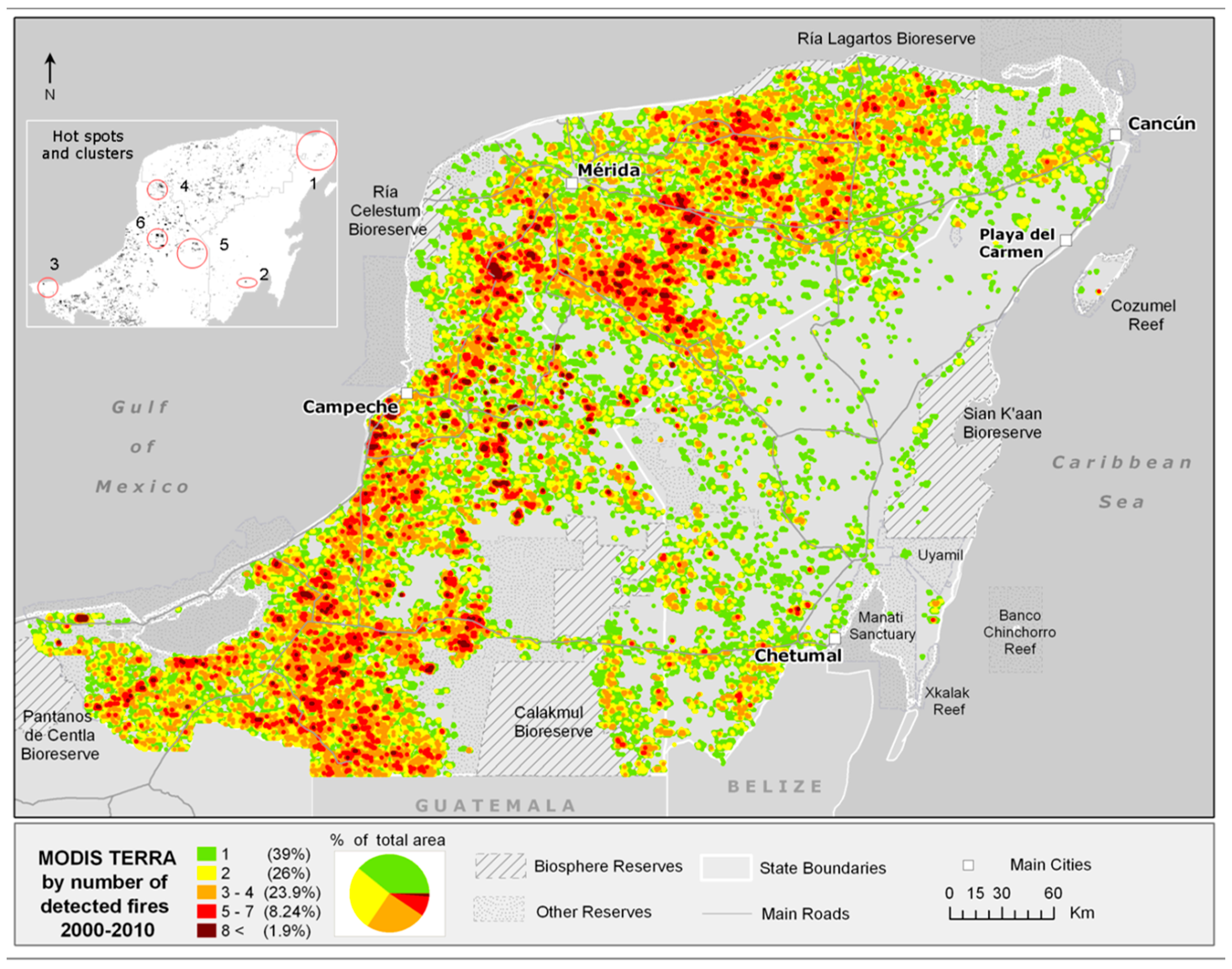
Figure 3.
Land change/persistence classes based on the CABS (2009) land cover maps.
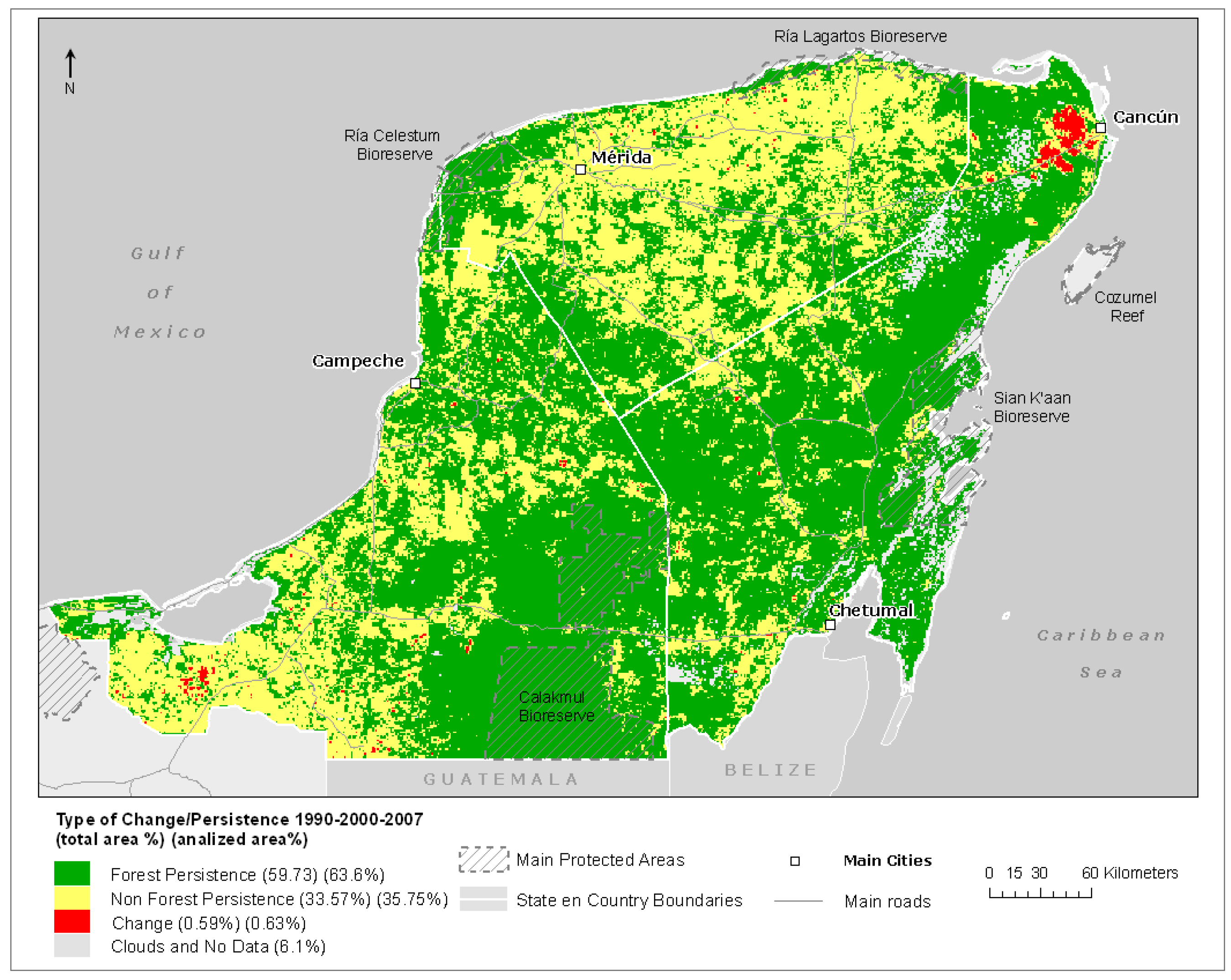
Figure 4.
Cumulative annual and 8-day frequency (counts) of fire occurrence (FIRE), 2000–2009 in the three-state Yucatán Peninsula: blue = morning purple = afternoon. Inset shows detail of intra-annual fire season for 2005.
Figure 4.
Cumulative annual and 8-day frequency (counts) of fire occurrence (FIRE), 2000–2009 in the three-state Yucatán Peninsula: blue = morning purple = afternoon. Inset shows detail of intra-annual fire season for 2005.

Figure 5.
Cross-tabulation of land change/persistence classes (Figure 1) and fire frequency (Figure 2).
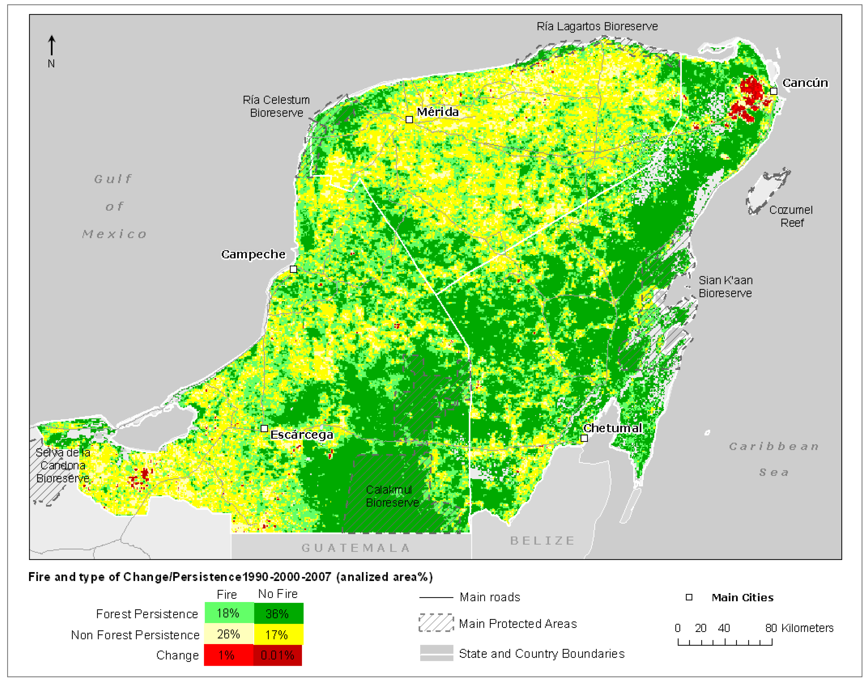
Figure 6.
Fire frequency aggregation for anthrome comparison (left) and Anthrome groups (right).

Figure 7.
Between group comparison: Fire frequency by anthrome groups boxplots (left). Within group comparison: Fire frequency boxplots within cropland anthrome (right).
Figure 7.
Between group comparison: Fire frequency by anthrome groups boxplots (left). Within group comparison: Fire frequency boxplots within cropland anthrome (right).
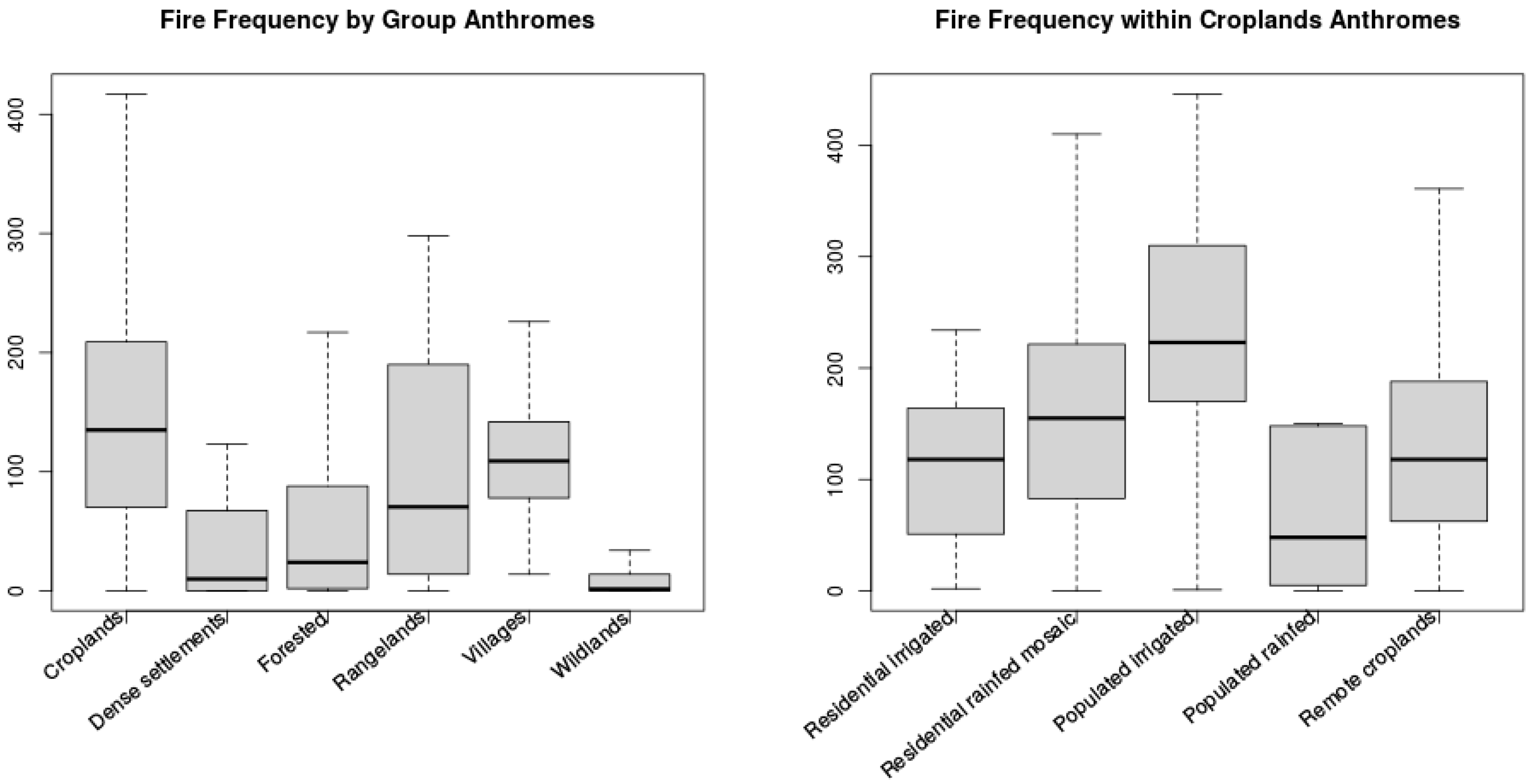
Table 1.
Cross-tabulation of fire occurrence and land change/persistence: row, column and total percentages per class. Preliminary interpretation matrix (extended/detailed legend for Figure 5).
Table 1.
Cross-tabulation of fire occurrence and land change/persistence: row, column and total percentages per class. Preliminary interpretation matrix (extended/detailed legend for Figure 5).
| Fire | No Fire | Row Total % | Total Study Area % | |
|---|---|---|---|---|
| Forest Persistence | 29.3% -Error resulting from database mismatch -Error of commission in MODIS Active Fire product -Error induced by aggregation of land cover data | 70.7% -Core areas of mature forest that have persisted for at least 17 years (1990–2007) -Protected areas with a predominance of mature forest -Areas of planned selective forest extraction that have not been extracted in 17 years or longer (under rotation management) | 100 | 54 |
| Non Forest Persistence | 60.8% -Areas where fire is used to convert from non-forest vegetation land covers to other non-forest vegetation land covers (e.g., agriculture to urban) -Areas of active non-forest land-uses -Error resulting from database mismatches | 39.18% -Areas under intensive land-uses that do not require land clearing for prolonged periods (e.g., citrus agriculture, urban) -Secondary vegetation of at least 10 years including forest not considered mature by CAB 2009. This can include forest regrowth (forest transition). -Forested areas of forest communities that have been extracted in the last 10 years and are growing back -Seasonal agricultural areas currently fallow (e.g., milpa) | 100 | 43 |
| Change (Forest to Non-Forest) | 86.0% -All land cover changes (conversion and some modification) preceded by land clearing by fire (i.e., deforestation) -Core forest areas that are heavily deforested with more intense use of land clearing by fire | 13.7% -Error of omission in MODIS Active Fire product -Error resulting from database mismatches -Land changes that do not require fire -Fringe areas that are cleared without fire after the core area has been cleared with fire -Fringe areas that are cleared with low intensity fire that is not detected by MODIS Active Fire product | 100 | 1 |
| Column TOTAL% | 45% | 36% | 100 | 100 |
Table 2.
Spatial multinomial logit model summary of trends. FP = forest persistence, NFP = non forest persistence, CH = change, INTE = Intercept, Odds = Odds ratio effects point estimates. This table contains only FIRE and CY variables, the full variable list is available in the Appendix A.
Table 2.
Spatial multinomial logit model summary of trends. FP = forest persistence, NFP = non forest persistence, CH = change, INTE = Intercept, Odds = Odds ratio effects point estimates. This table contains only FIRE and CY variables, the full variable list is available in the Appendix A.
| CAT | REF | INTE | CY | FIRE | Odds CY | Odds FIRE |
|---|---|---|---|---|---|---|
| CH (3) | FP (1) | −4.67 | −3.55 | 1.92 | 0.03 | 6.79 |
| NFP (2) | −6.07 | −3.46 | 0.20 | 0.03 | 1.22 | |
| CH Average | −5.37 | −3.50 | 1.06 | 0.03 | 4.00 | |
| FP (1) | CH (3) | 4.67 | 3.55 | −1.92 | 34.66 | 0.15 |
| NFP (2) | −4.38 | 0.07 | −1.72 | 1.07 | 0.18 | |
| FP Average | 0.15 | 1.81 | −1.82 | 17.87 | 0.16 | |
| NFP (2) | CH (3) | 9.05 | 3.48 | −0.20 | 32.43 | 0.82 |
| FP (1) | 4.38 | −0.07 | 1.72 | 0.94 | 5.59 | |
| FP Average | 6.71 | 1.71 | 0.76 | 16.68 | 3.20 |
Table 3.
Between-anthromes Tukey pairwise comparison for the negative binomial models with fire count and anthromes groups. Note that the reference variable is in italic.
Table 3.
Between-anthromes Tukey pairwise comparison for the negative binomial models with fire count and anthromes groups. Note that the reference variable is in italic.
| Pairwise Comparison | Coefficients | Standard Error | t-Stat | p-Values |
|---|---|---|---|---|
| Dense settlements–Croplands | −1.38688 | 0.43059 | −3.2209 | 0.0121 |
| Forested–Croplands | −0.92198 | 0.06997 | −13.1762 | 0 |
| Rangelands–Croplands | −0.35406 | 0.26321 | −1.3452 | 0.7146 |
| Villages–Croplands | −0.28199 | 0.32807 | −0.8595 | 0.9435 |
| Wildlands–Croplands | −2.29463 | 0.19565 | −11.7283 | 0 |
| Forested–Dense settlements | 0.46491 | 0.42934 | 1.0828 | 0.8616 |
| Rangelands–Dense settlements | 1.03282 | 0.49872 | 2.0709 | 0.2552 |
| Villages–Dense settlements | 1.10489 | 0.53579 | 2.0622 | 0.2593 |
| Wildlands–Dense settlements | −0.90775 | 0.4666 | −1.9454 | 0.3214 |
| Rangelands–Forested | 0.56791 | 0.26118 | 2.1744 | 0.2076 |
| Villages–Forested | 0.63999 | 0.32644 | 1.9605 | 0.3129 |
| Wildlands–Forested | −1.37266 | 0.1929 | −7.1159 | 0 |
| Villages–Rangelands | 0.07207 | 0.41346 | 0.1743 | 1 |
| Wildlands–Rangelands | −1.94057 | 0.31874 | −6.0882 | 0 |
| Wildlands–Villages | −2.01264 | 0.37409 | −5.3801 | 0 |
Table 4.
Within-anthrome Tukey pairwise comparisons using the negative binomial models with fire count and anthromes croplands categories. Note that the reference variable is in italic.
Table 4.
Within-anthrome Tukey pairwise comparisons using the negative binomial models with fire count and anthromes croplands categories. Note that the reference variable is in italic.
| Pairwise–Comparison | Coefficients | Standard Error | t-Stat | p-Values |
|---|---|---|---|---|
| Populated rainfed cropland–Populated irrigated cropland | 0.25239 | 0.22555 | 1.119 | 0.7646 |
| Remote croplands–Populated irrigated cropland | 0.572 | 0.25835 | 2.214 | 0.1453 |
| Residential irrigated cropland–Populated irrigated cropland | −0.61118 | 0.41094 | −1.4873 | 0.5244 |
| Residential rainfed mosaic–Populated irrigated cropland | 0.08091 | 0.22337 | 0.3622 | 0.9955 |
| Remote croplands–Populated rainfed cropland | 0.31961 | 0.14756 | 2.166 | 0.1615 |
| Residential irrigated cropland–Populated rainfed cropland | −0.86357 | 0.352 | −2.4533 | 0.0827 |
| Residential rainfed mosaic–Populated rainfed cropland | −0.17148 | 0.07017 | −2.4437 | 0.0848 |
| Residential irrigated cropland–Remote croplands | −1.18318 | 0.37387 | −3.1647 | 0.0105 |
| Residential rainfed mosaic–Remote croplands | −0.49109 | 0.14421 | −3.4054 | 0.0043 |
| Residential rainfed mosaic–Residential irrigated cropland | 0.69209 | 0.35061 | 1.974 | 0.2396 |
© 2017 by the authors. Licensee MDPI, Basel, Switzerland. This article is an open access article distributed under the terms and conditions of the Creative Commons Attribution (CC BY) license (http://creativecommons.org/licenses/by/4.0/).
Share and Cite
MDPI and ACS Style
Millones, M.; Rogan, J.; II, B.L.T.; Parmentier, B.; Harris, R.C.; Griffith, D.A. Fire Data as Proxy for Anthropogenic Landscape Change in the Yucatán. Land 2017, 6, 61. https://doi.org/10.3390/land6030061
AMA Style
Millones M, Rogan J, II BLT, Parmentier B, Harris RC, Griffith DA. Fire Data as Proxy for Anthropogenic Landscape Change in the Yucatán. Land. 2017; 6(3):61. https://doi.org/10.3390/land6030061
Chicago/Turabian StyleMillones, Marco, John Rogan, B.L. Turner II, Benoit Parmentier, Robert Clary Harris, and Daniel A. Griffith. 2017. "Fire Data as Proxy for Anthropogenic Landscape Change in the Yucatán" Land 6, no. 3: 61. https://doi.org/10.3390/land6030061
Note that from the first issue of 2016, this journal uses article numbers instead of page numbers. See further details here.