Article

Retrieving the National Main Commodity Maps in Indonesia Based on High-Resolution Remotely Sensed Data Using Cloud Computing Platform

1
Tropical Biodiversity Conservation Program, Department of Forest Resources Conservation and Ecotourism, Faculty of Forestry, IPB University (Bogor Agricultural University), Kampus IPB Darmaga Bogor 16680, Indonesia
2
Department of Forest Resources Conservation and Ecotourism, Faculty of Forestry, IPB University (Bogor Agricultural University), Kampus IPB Darmaga Bogor 16680, Indonesia
3
Faculty of Agriculture, University of Teuku Umar, Meulaboh, Aceh Barat, Aceh 23681, Indonesia
4
Natural Resources and Environmental Management Studies Program, Graduate School of IPB University (Bogor Agricultural University), Kampus IPB Baranangsiang Bogor 16129, Indonesia
*
Author to whom correspondence should be addressed.
Land 2020, 9(10), 377; https://doi.org/10.3390/land9100377
Submission received: 9 September 2020 / Revised: 5 October 2020 / Accepted: 6 October 2020 / Published: 8 October 2020

Abstract

:
Indonesia has the most favorable climates for agriculture because of its location in the tropical climatic zones. The country has several commodities to support economics growth that are driven by key export commodities—e.g., oil palm, rubber, paddy, cacao, and coffee. Thus, identifying the main commodities in Indonesia using spatially-explicit tools is essential to understand the precise productivity derived from the agricultural sectors. Many previous studies have used predictions developed using binary maps of general crop cover. Here, we present national commodity maps for Indonesia based on remote sensing data using Google Earth Engine. We evaluated a machine learning algorithm—i.e., Random Forest to parameterize how the area in commodity varied in Indonesia. We used various predictors to estimate the productivity of various commodities based on multispectral satellite imageries (36 predictors) at 30-meters spatial resolution. The national commodity map has a relatively high accuracy, with an overall accuracy of about 95% and Kappa coefficient of about 0.90. The results suggest that the oil palm plantation was the highest commodity product that occupied the largest land of Indonesia. However, this study also showed that the land area in rubber, rice paddies, and cacao commodities was underestimated due to its lack of training samples. Improvement in training data collection for each commodity should be done to increase the accuracy of the commodity maps. The commodity data can be viewed online (website can be found in the end of conclusions). This data can further provide significant information related to the agricultural sectors to investigate food provisioning, particularly in Indonesia.

Graphical Abstract

1. Introduction

Agricultural industries are an integral part of the Earth’s ecology and play a significant role in human livelihoods [1,2]. Indonesia has the most favorable climates in the world for agriculture [2]. Indonesia’s wealth of natural resources and a range of goods is a significant and indispensable commodity for its economy. The commodities contribute around 60 per cent of all exports from Indonesia. Following the healthy growth shown by exports to Indonesia over the years, exports from Indonesia are estimated at $158 billion annually as of 2017 [3]. Indonesia has several commodities that support the economics growth such as palm oil, rubber, coffee, cacao, and paddy. Existing croplands not only feed this country’s population but also play a key role in the nations’ economic income, with many food products such as rice, coffee, tea, cocoa, and palm oil exported to many countries around the world [2]. The main crop is rice, and the Indonesian government has emphasized increasing the national agricultural self-sufficiency by developing the infrastructures and subsidies for rice production [4]. Oil palm plantation contributes significantly to the economies of Indonesia and Malaysia through private corporations, state-owned companies, and small-landholders, who supply 85% of global palm oil exported in both countries [5]. However, in Indonesia, oil palm plantations were linked to significant deforestation during the 1990s and 2000s [6,7]. Furthermore, Indonesia boasts the world’s largest rubber plantations, with 3.61 million hectares of total land area in their production [8]. In Indonesia, rubber plantations are distributed from the west to the east in 30 provinces. Besides, Indonesia is also the world’s third-largest coffee producer and exporter, after Brazil and Vietnam. Geographically, the production of coffee is distributed across the entire country. Whilst the South Sumatra is the center of Robusta coffee bean production and Arabica beans are mostly grown in Northern Sumatra, coffee is grown across all the major Indonesian islands; coffees beans from Java, Bali, Sulawesi, Flores, and Indonesian Papua are all sold on domestic and international specialty coffee markets [9,10]. In addition, the cacao bean is also one of Indonesia’s most significant agricultural export products that have experienced massive growth over the past 25 years, driven by a rapid expansion in the participation of smallholder farmers [11].
Understanding the precise spatial distribution of cropland areas, and the ability to map any field, irrespective of its size, with sufficiently high resolution above 30 m and over very large spatial areas with high precision is of great importance. This is because it aids in observing, accessing, and planning the global food and water sustainability scenarios in an increasingly interconnected world [2,12,13]. Other studies have predicted the global cropland extent across Eurasia, the United States, and Australia using Landsat 8 imageries [2,13,14,15]. The definition of croplands used in those studies was lands grown with plants harvested for food, feed, and fiber, including both annual crops and continuous plantations such as coffee, tea, rubber, cocoa, and oil palms. Cropland fallows is defined as cultivation-equipped areas including plantations and those not grown for a season or two are included in the cropland category [12,13,14]. However, the previous study only distinguished the cropland into binary maps (i.e., cropland and non-cropland) with the general-commodities extent using remotely sensed data.
Currently, the ability to distinguish cacao agroforestry areas with a multi-strata canopy, using optical reflectance and vegetation indices, has not proved successful [16]. Delineation of cacao agroforestry areas using Sentinel-1 imageries has been successfully used in Cameroon with relatively good results to produce cacao maps (OA: 88.8%; [17]). Paddy rice classification was performed by combining Landsat and Synthetic Aperture Radar (SAR) data through machine learning approaches [18]. Furthermore, the difficulty of predicting paddy field areas largely arises from the related spectral characteristics between paddy rice and other land cover types, as well as frequent clouds and cloud shadows in rice-growing areas. Existing efforts have implemented various data sources and approaches for mapping paddy rice, and the methods can generally be divided into three categories, namely image statistics-based, time series, and phenology-pixel-based mixed approaches [4,19,20]. Previous research primarily focused on the distinction between rubber trees and either deciduous or evergreen forest depending on the location [21,22]. Rubber plantations were identified by vegetation indices of Landsat imageries using support vector machine [23]. Nevertheless, for a tropical country such as Indonesia, instead of evergreen trees being spectrally identical in properties as rubber trees and croplands such as oil palm trees, resulting in misclassifications of these three forms of vegetation. This may pose a problem because rubber has very similar growth requirements as palm oil, and thus both crops are grown in the same geographic areas even though either active or passive sensor imageries have been used to distinguish these crops [23]. Several recent studies have developed advanced classification algorithms and imagery data from high-resolution passive sensors to enhance the classification of small-landholder coffee areas [24,25,26]. Utilization of machine learning algorithms to identify shade-grown coffee areas has been evaluated in Nicaragua [27]. However, it has long proven challenging to detect shade-grown coffee precisely using remotely sensed data. Many studies across the tropics have conducted mapping of oil palm land cover using remote satellite sensing data [6,28,29,30]. The methods to distinguish oil palm cover from other vegetative community types can generally be divided into two categories: image and phenology-based approaches [28]. Shade-grown coffee also retrieved using Landsat 8 imageries, topographical data from Shuttle Radar Topography Mission (SRTM), and precipitation data (CHIRPS) through Random Forest algorithm [27]. Therefore, multispectral imageries associated with the digital elevation model and physiographic or geophysical data can be used to retrieve commodity covers. Here, we present the commodity crops (i.e., oil palm, rubber, rice, cacao, and coffee) in one classification rule-set based on very-high satellite imageries (30-m) using the cloud computing platform.
In this decade, the cloud computing platform has been widely used to retrieve land cover maps in the planetary scale—i.e., Google Earth Engine (GEE). Google Earth Engine is a cloud-based geo-spatial analysis platform that delivers massive computing capabilities to address a variety of high-impact societal issues including deforestation, drought, disaster, disease, food security, water management, climate monitoring, and environmental protection [31]. In this study, we used the Google Earth Engine Platform to generate a good quality of satellite imageries and perform the machine learning classification to predict the commodity maps across Indonesia.

2. Materials and Methods
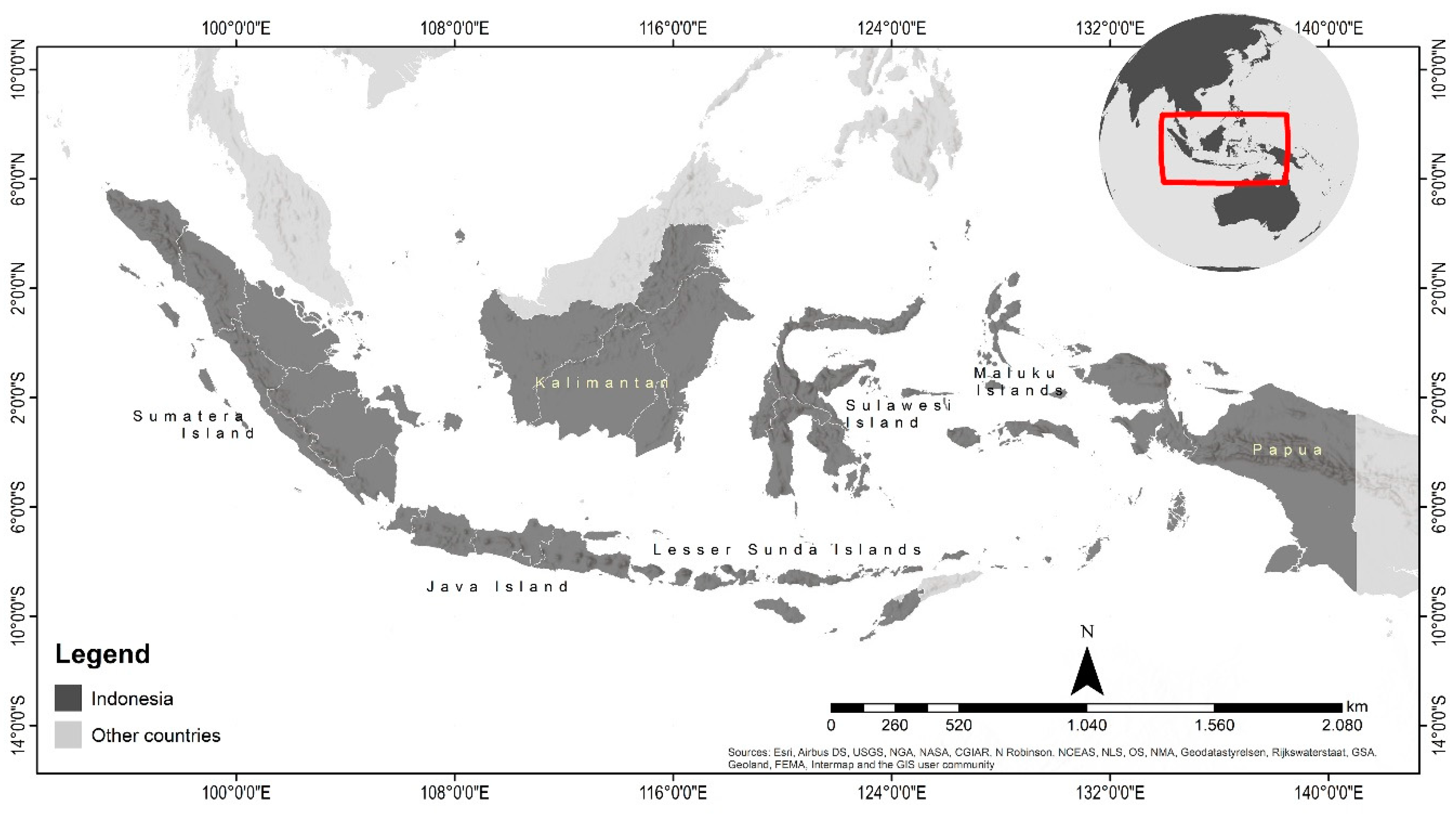
2.1. Study Area

This study was carried out in Indonesia (Figure 1) —a tropical country with the potential to support agricultural and plantation production of commodity crops [32]. Indonesia is the fourth most populous country with the largest Muslim population in the world with a total of 267,026,366 people [33]. High demand of food and economics due to population density is connected to agricultural land [32].

2.2. Training Data

We used a variety of databases to retrieve commodity identification training for the model input. A database of five main commodities—i.e., oil palm, rubber, coffee, cacao, and paddy was compiled from the following sources: (1) Biodiversity records from the Global Biodiversity Information Facility database (s; www.gbif.org); keywords “Hevea brasiliensis”, “Elaeis guineensis”, ”Coffea arabica”, ”Coffea canephora”, “Theobroma cacao”, and “Oryza sativa”; (2) the database for rice paddy cover in Indonesia created by The Ministry of Agriculture; (3) Industrial oil palm extent of Indonesia; digitized from Austin et al., (2017); (4) Field survey in four pilot locations—i.e., Aceh Province, South Tapanuli Regency, Pelalawan Regency, and Sintang Regency were also used for training data. Point acquisition to obtain commodity information by survey was conducted in 2018–2019 during the dry season; we also conducted interviews with local people to identify dominant land cover types in the areas. Geographic coordinates were recorded in decimal degrees, based on the WGS 1984 datum. We also used 7621 points from other land cover types data (22 classes), retrieved from the Ministry of Environment and Forestry of Indonesia.
Data filtering was essential for further analyses due to the records from the global database, GBIF in particular may contain potential errors or duplicated data. Records from all of the databases were integrated or merged into a training dataset. Records of commodity with the dataset without any hard facts, including relevant or detailed descriptions, were excluded from analysis. For this study, this resulted in 236 data points for coffee (both arabica and robusta), 29 data points for cacao, 52 for rubber, 294 rice paddies, 504 points of oil palm, and 7621 points of other land cover types. Specific information related to the other land cover types for the training data consists of: 1683 data points for dryland primary forest, 1651 data points for dryland secondary forest, 66 for primary mangrove forest, 231 for primary peat-swamp forest, 192 data points for plantation forest, 590 points of shrub, 215 points of plantation, 94 points of settlement, 186 points of bare land, 111 points of savanna, 149 points of waterbody, 65 points of secondary mangrove forest, 262 points of secondary peat-swamp forest, 309 points of mixture of shrub and swamp, 398 points of dryland agriculture, 1088 points of mixture dryland agriculture, 188 points of wetland cultivation, 37 points of cultivated pond, 10 points of built-up area, 9 points of transmigration area, 27 points of mining, and 60 points of swamp.

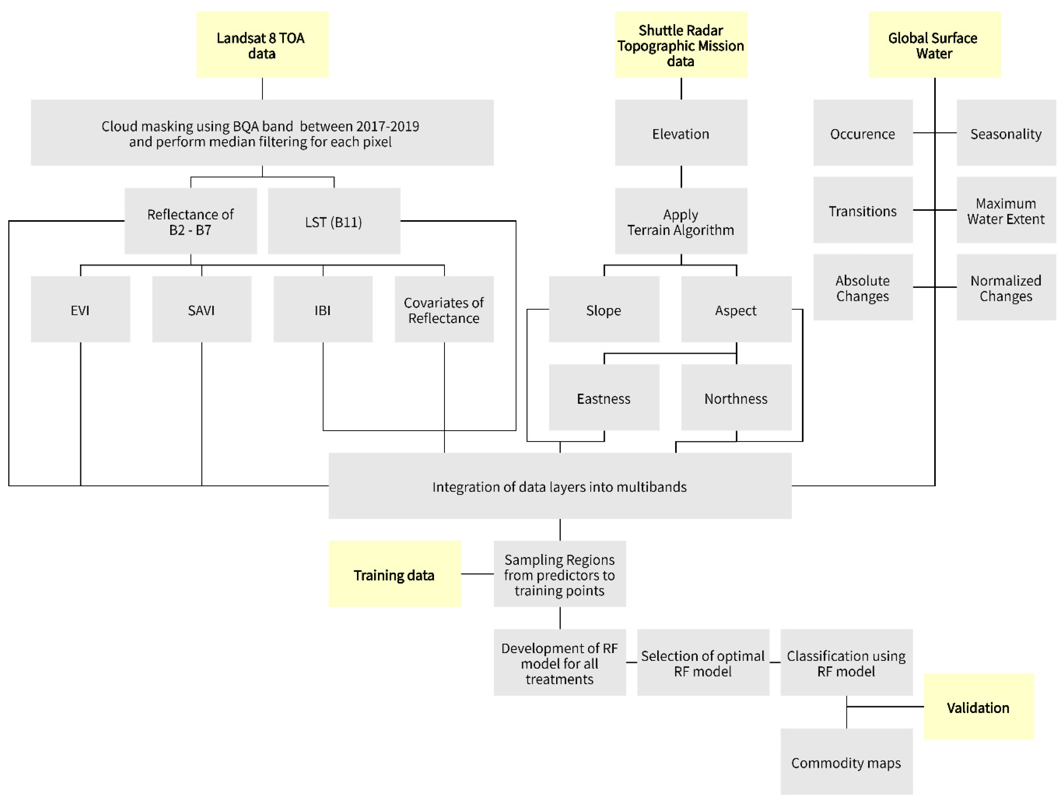
2.3. Features Derives

This study used a total of 36 features from satellite imageries—i.e., Landsat 8 imageries, Shuttle Radar Topographic Mission (SRTM) data, and Joint Research Center (JRC) global surface water data at 30 m × 30 m spatial resolution to identify the commodities. Table 1 shows the details of the dataset used in this study.
We used reflectance of Landsat 8 top of atmosphere (TOA) with Tier 1 level data where the data was already geo-registered with root mean square error (RMSE) less than 12 m resolution which represented the best quality imagery available for the collected data [34]. Cloud-masking using Quality Assessment band (BQA) and filter statistics by pixels (i.e., median) over the period of Landsat 8 TOA reflectance imageries were performed before further analysis within The Google Earth Engine. The research was also carried out using moving average lag time of 1-year analysis of images collection to determine the recent period of Landsat 8 due to cloud cover issues in the humid tropical region [35]. Furthermore, we used images from January 1st 2017 to December 31st 2019 to represent the 2018 data with clear cloud cover.
EVI represents an optimized vegetation index which has the ability to improve vegetation monitoring by reducing atmospheric disturbance and canopy background signal. EVI is calculated using the following equation [36]:
E V I = G × N I R R E D N I R + C 1 × R E D   C 2   × B L U E + L ,
where NIR or RED or BLUE are spectral reflectance (atmospherically corrected) of near-infrared, red, and blue wavelengths respectively, C1 and C2 are the coefficient of the aerosol resistance with the values of 6 and 7.5, G represents gain factor (2.5), and L refers to 1 [36].
SAVI represents a vegetation index with reduced effects of soil brightness in areas where vegetation density is sparse or low [37]. This index is calculated as the following equation:
S A V I = ( 1 + L ) ×   N I R R E D N I R + R E D + L ,
where NIR and RED are spectral reflectance (atmospherically corrected) of near-infrared and red wavelengths and L refers to soil brightness correction factor (0.5).
IBI is proposed for the rapid extraction of built-up land objects in remotely sensed data or non-vegetation retrieval [38]. IBI is calculated as:
I B I a = 2   ×   S W I R 1 S W I R 1 × N I R ,
  I B I b = N I R N I R + R E D +   G R E E N G R E E N + S W I R 1   ,
  I B I =   I B I a I B I b I B I a +   I B I b   ,
where SWIR1 and GREEN are spectral reflectance (atmospherically corrected) of shortwave-infrared (1.57–1.65 µm) and green wavelengths. IBI (Equation (5)) is the normalized difference ratio between IBIa (Equation (3)) and IBIb (Equation (4)).
Interspecific covariate has been calculated to represents more statistics variation in the machine learning algorithm for commodity detection. Covariate between two-bands can be calculated using the following equation:
N D ( B A N D i , B A N D j ) = B A N D i B A N D j B A N D i + B A N D j ,
where BANDi or BANDj represents spectral reflectance of Landsat 8 (atmospherically corrected) for blue, green, red, near-infrared, shortwave-infrared 1, and shortwave-infrared 2. Thus, this variable is the normalized difference of each multispectral band in Landsat 8.

2.4. Commodity Cover Prediction

To identify the national commodity cover in Indonesia—i.e., oil palm, rubber, coffee, cacao, and rice paddies, we used machine learning classification through the Random Forest (RF) algorithm within the multiclass classification (total of 27 classes) in the Google Earth Engine Platform. GEE has 10 classifiers with different algorithm to estimate a pixel-based classification—i.e., CART, RF, Minimum Distance, GMO MaxEnt, Naive Bayes, SVM, Perceptron, IKPamir, and Winnow [29]. Random Forest gives the best performance from other classifiers [41]; therefore, we choose this algorithm to predict commodity classes. A Random Forest classifier provides an ensemble model that effectively distinguishes spectrally similar agriculture land and forest cover by generating multiple trees from training data and its predictors [27,31,42]. Many studies have investigated the performance of the RF algorithm to identifying land cover from hyperspectral, multispectral imageries, and digital elevation model data as well [43,44,45].
Random Forest classifiers with high variance and low bias perform by growing the forest to a user-defined number-of-trees [42]. This study evaluated various RF models using different parameterization of the number-of-trees (N); i.e., N = 25, N = 50, N = 100, and N = 500 to obtain the best model from the various parameterization of RF classifiers. We use 36 number of features derived from Landsat 8 imageries and the digital elevation model as well. The number of variables per split has been defined as root square of the number of features; i.e., 6. We describe each of these methods in the following flowchart (Figure 2).

2.5. Model Evaluation

Accuracy assessment for the overall model was measured by the error matrices which were used to estimate the user’s accuracy (the accuracy of classification despite commission error) and the producer’s accuracy (the accuracy of classification despite omission error). Then, we provided a Kappa coefficient to examine the goodness of the predictions relative to validated reference data [46]. However, the Kappa coefficient has come under recent question as a useful metric for accuracy assessments [47]. Quantity disagreement is the amount of difference between the reference categories and the classified categories that is due to the less than perfect match in the proportions of the categories. Allocation disagreement is defined as the amount of difference between the reference categories and the classified categories that is due to the less than maximum match in the spatial allocation of the categories, given the proportions of the categories in the reference and comparison maps. The total disagreement is the sum of quantity disagreement and allocation disagreement [47]. We also compare the statistics of total areas for each commodity with reference data from the Statistics Bureau of Indonesia by province [8]. We perform zonal statistics for each commodity by provincial administration to calculate total of commodity area.
The variable importance can be calculated generally using mean decrease in accuracy (MDA) or mean decrease in Gini (MDG) [48]. The mean decrease in Gini coefficient estimates each variable contribution to the homogeneity of the nodes [14]; besides MDA coefficient is the average change in accuracy across the forest [49]. Many studies used the MDG to calculate the variable importance [14,49,50]. The MDG provides the good robustness while the MDA tend to unstable to small perturbations of the dataset [49,51]. We estimated the relative importance of each predictor to the model using the percent contribution and variable importance for the best model using mean decrease in Gini [42]. We also investigated the response curves of the 4th most important variables to explore how the predictors affected the commodity prediction.

3. Results

3.1. Accuracy Assessment

Generally, the RF algorithm with 100 number of trees gives the highest accuracy based on overall accuracy and Kappa coefficient (OA = 95.2% and κ = 0.90; Table 2). The best RF model (N = 100) has relatively strong agreement based on κ and OA [52].
Cacao has the lowest value of producer’s accuracy (PA) ranging from 39.6% to 52.2%. Otherwise, oil palm has the highest PA ranging from 78.9% to 93.2%. Besides, oil palm also has the lowest user’s accuracy (UA) values ranging from 58.4% to 85.8%. Coffee has the highest value of UA ranging from 83.3% to 97.9% (Table 3).
Nevertheless, the standard Kappa coefficient had some considerable conceptual problems [53]—thus we also calculate quantity and allocation disagreement [47].
Figure 3 summarizes the omission disagreement, agreement, and commission disagreement by category for each Random Forest 2019 commodity maps. Vertical axis shows the categories while the horizontal axis shows the number of validation observations. The Random Forest algorithm with number of trees 100 (Figure 3C) has the least disagreement both commission and omission. Figure 3 shows that the omission disagreement is greater than the commission disagreement for the most of commodity (i.e., rubber, oil palm, coffee, cacao, and also paddy in Figure 3B,C), therefore those commodities were underestimated by all methods. In contrast, paddy in Figure 3A was overestimated.

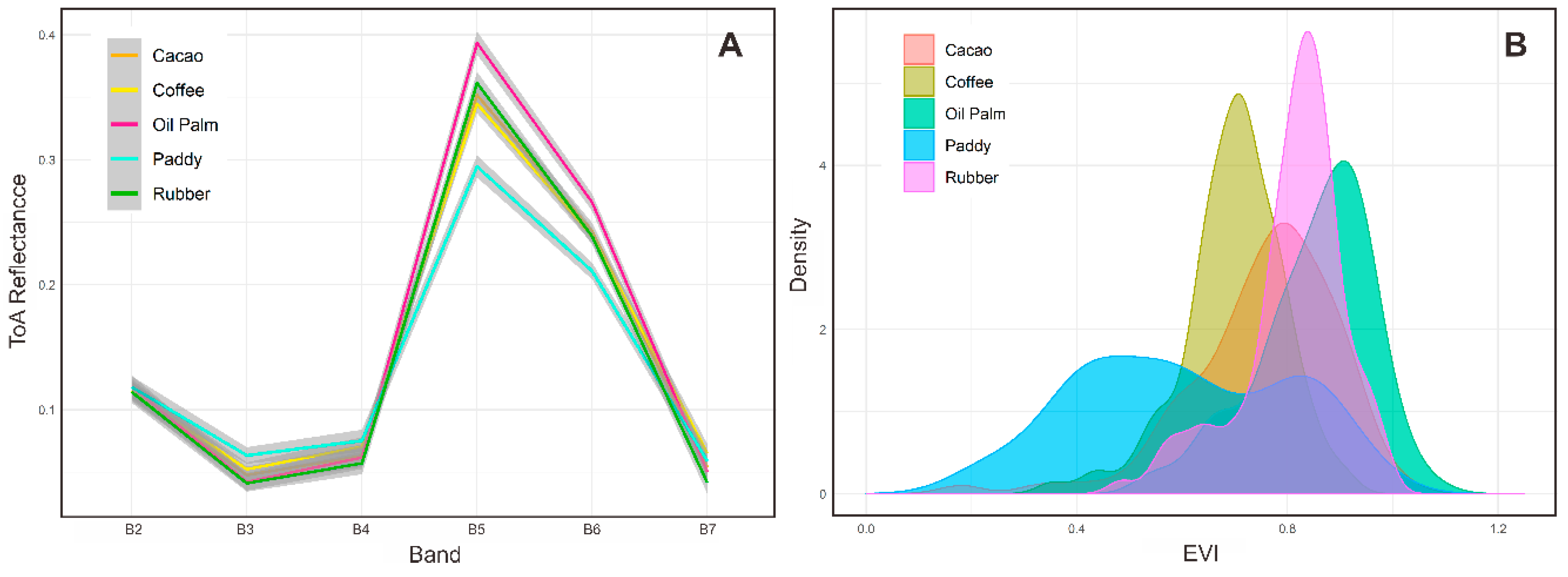
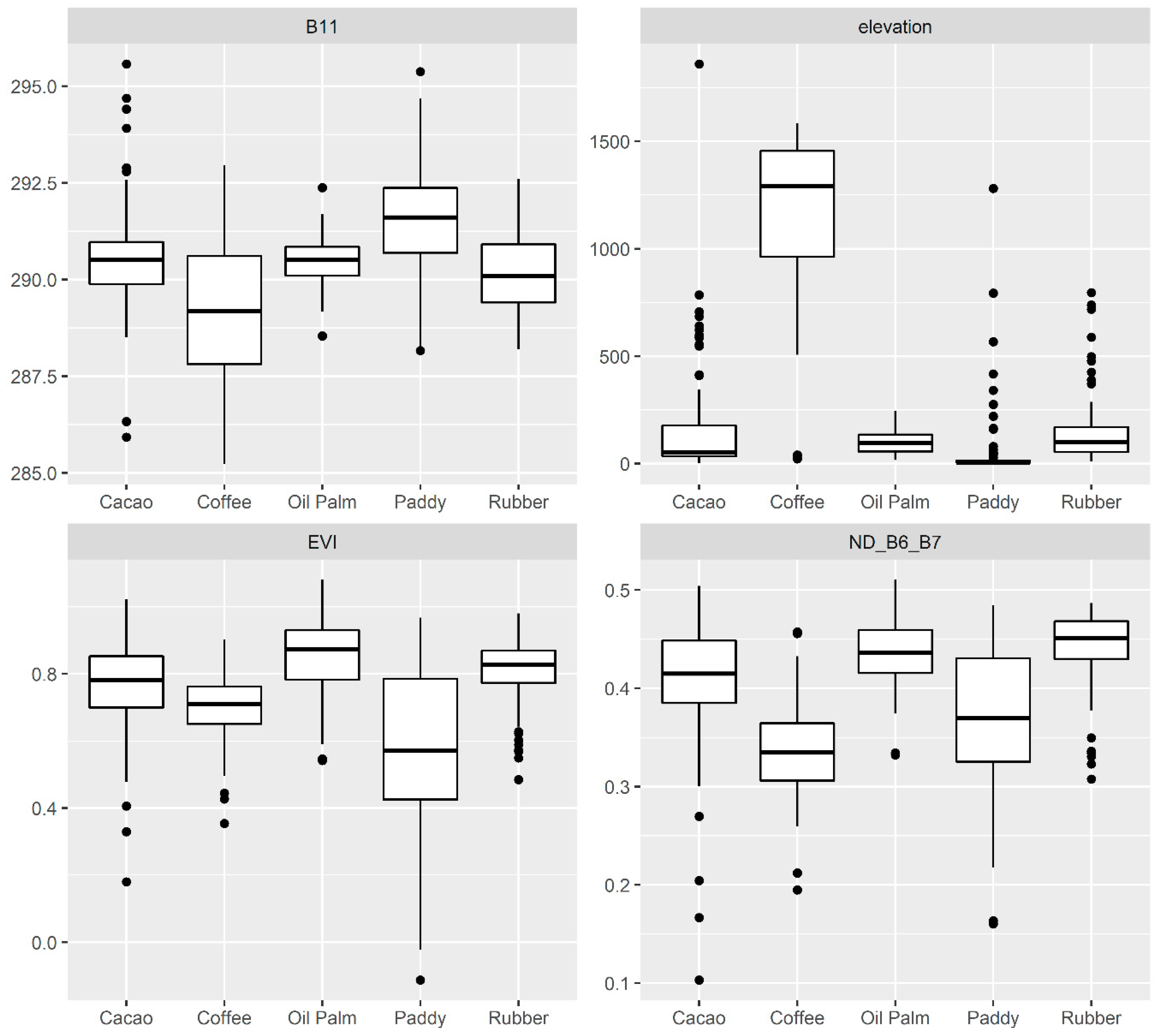
3.2. Spectral Characteristics

We can see a relatively contrast characteristic of commodity from Near Infra-Red Band (NIR; B5) and Short-Wave Infra-Red Band (SWIR; B6). The result shows that coffee, cacao, and rubber have a similar spectral characteristic from Landsat 8 multi-spectral bands (in moderate values of near infra-red range). Moreover, oil palm has a highest spectral value in near infra-red range. Otherwise, paddy has the lowest spectral value of B5 (Figure 4).
The results show that elevation, land surface temperature (B11), covariate of B6 and B7 (ND_B6_B7), and EVI were the four most important variables by mean decrease in Gini coefficient values (325, 75, 52, and 38, respectively). EVI was the most importance variable in commodity maps of Indonesia—therefore, we analyze spectral characteristic from EVI for various commodities (Figure 5).
Elevation predictor shows the higher discrimination between the commodities (Figure S1). Coffee is found at higher altitude areas (1151 ± 389) m asl. Besides, cacao, oil palm, paddy, and rubber were found in relatively lower elevation (117 ± 161) m asl than coffee. In the land surface temperature perspectives, paddy was suitable to grow in high temperature areas (291.50 ± 1.27) Kelvin. Otherwise, coffee plantation has the lowest temperature (289.20 ± 1.75) Kelvin than the other commodities. The average of EVI value for oil palm, rubber, cacao, coffee, and paddy were 0.85, 0.81, 0.76, 0.70, and 0.59, respectively.

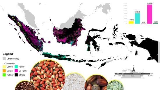
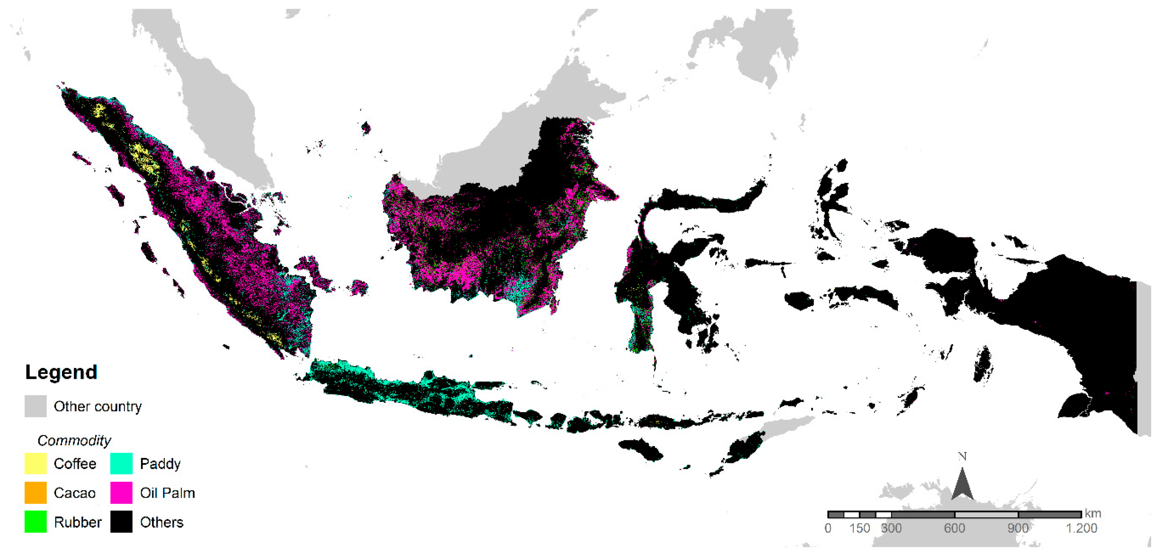
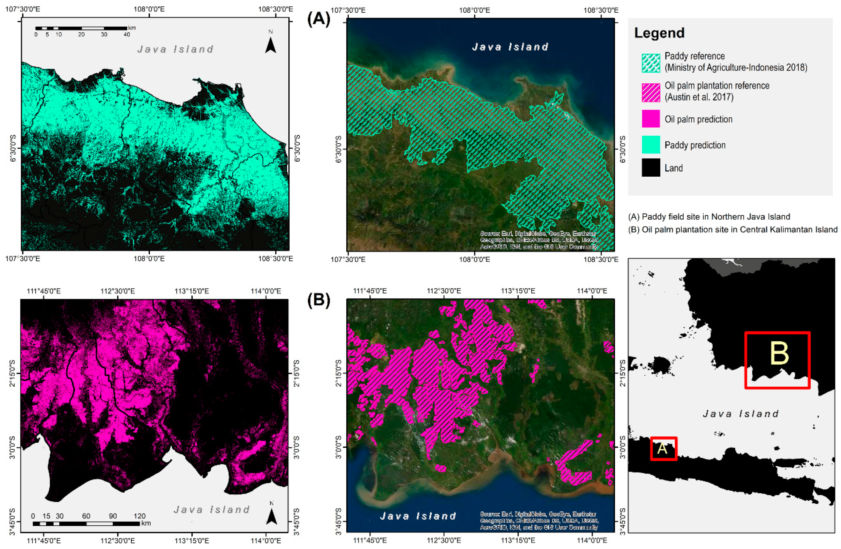
3.3. Spatial Distributions of Commodity Maps

The results show that generally, 6.5% (25.39 million ha) of the total geographic area was net commodity of 2019) with the total area of coffee, cacao, rubber, paddy, and oil palm were 1.96 million ha, 96.98 thousand ha, 279.59 thousand ha, 8.15 million ha, and 14.89 million ha, respectively. The commodities were rapidly growing in Sumatera, Kalimantan, and Java regions (Figure 6).
Oil palm plantation was the most dominant commodity than the others, particularly in Sumatera and Kalimantan. Meanwhile, Java Island was one of the most suitable regions for paddy growth. North Sumatera Province has the highest total areas of coffee, rubber, and cacao plantations covering 748.43 thousand ha, 61.06 thousand ha, and 32.17 thousand ha, respectively. East Java Province has the highest total areas of paddy field (1.21 million ha). Riau Province has the highest total areas of oil palm plantation (2.51 million ha). However, research on the comparisons of coffee, rubber, and cacao with the spatial reference data had not been carried out due to the lack of data (Figure 7).

4. Discussion

Google Earth Engine is a cloud computing platform with the ability to carry out the machine learning classifications and perform pre-processing big-data computing of multispectral satellite imageries [18,29]. This study shows that various types of commodity, such as coffee, cacao, oil palm, rubber, and paddy plantations can be mapped at a high spatial resolution of 30 m. Furthermore, the results retrieved with the Random Forest algorithm, which is one of the machine learning approaches, outperformed prior studies. This research realized that the model has relatively high accuracy (OA = 95% and κ = 0.90) for the Random Forest algorithm with N value of 100. Moreover, it also provides a good result to discriminate various types of the commodity using multispectral satellite imageries. The results of this study were also compared with the official reference data from Statistical Bureau of Indonesia [8] for the oil palm and paddy commodities and also from the previous studies used to identify the commodity [29,54]. The difference between the study’s oil palm plantation map (14,896,964 ha) with the areas from BPS (14,677,561 ha) was approximately 1%; with the highest value found in Riau Province as the center of oil palm commodity province both for smallholder farmers and industrial plantation [55]. Furthermore, the difference between our paddy rice field map (8,152,435 ha) with paddy rice field areas from BPS (10,677,887 ha) was 24%. This result was still underestimated towards reference data from BPS. However, this result was still underestimated towards reference data from BPS, therefore the similar spatial characteristics between maps and other reference data shows East Java as the highest total area of paddy rice field in Indonesia as shown in Figure S2 [8,56,57,58].
This study shows a lower omission error of the oil palm plantation than the prior research carried out by Lee et al. [29] (PA = 88% vs. PA = 93% in our estimation). However, the study of [29] has a slightly lower commission error of oil palm plantation than this study’s estimation (UA = 88% vs. UA = 86% in our estimation). According to the [54], this study has higher performances, both producer and user accuracies (PA = 82% vs. PA = 90% in our estimation and UA = 65% vs. UA = 94% in our estimation). This study also shows the higher producer’s and user’s accuracies of coffee plantation than the previous research (PA = 86% compared to 82% in Kelley’s et al. [27]. data and UA = 98% compared to 80% in Kelley’s et al. [27] dataset). Nevertheless, this study’s results for cacao plantation still has a poor result based on comparison from the previous study (PA = 51% compared to 96% in Numbisi’s et al. [17] dataset). However, this research has a higher user’s accuracy of cacao plantation (UA = 95% compared to 86% in Numbisi’s et al. [17] dataset). The study also shows higher omission and commission errors of rubber plantation compared to Kou et al. [21]; PA = 95% vs. PA = 68% in our estimation and UA = 91% vs. UA = 87% in our estimation. The high omission error in cacao and rubber plantations suggests that there was still a lack of training data for those commodities.
To improve the accuracy of the commodity maps, further field works for collecting more training data of commodity needs to be carried out, particularly for cacao, rubber, and coffee. The previous study has suggested that a large number of representative samples will increase the performances of the model [59]. Compiling secondary data from the governments (e.g., the Ministry of Agriculture or the Ministry of Environment and Forestry) and defining the consensus of its data within our data (i.e., commodity maps) also should be carried out—therefore, a general agreement of the commodity data can be revealed.

5. Conclusions

The study successfully produced the high spatial resolution of 30 m for commodity maps in Indonesia region. The results show that the total geographic area of the net commodity in 2019 was 6.5% (25.39 million ha) with coffee, cacao, rubber, paddy, and oil palm covering 1.96 million ha, 96.98 thousand ha, 279.59 thousand ha, 8.15 million ha, and 14.89 million ha, respectively. The product has relatively high accuracy, with an overall accuracy of 95% and a Kappa coefficient of 0.90. However, several commodities were still further underestimated due to lack of training samples. Therefore, improvement in training data collection for each commodity needs to be carried out to increase the accuracy of the commodity maps. The recent commodity data can be viewed at http://lulcc.ipb.ac.id/map/frontend/home.

Supplementary Materials

The following are available online at https://www.mdpi.com/2073-445X/9/10/377/s1, Figure S1: The importance of input variables for the commodity maps by mean decrease Gini coefficient values. BX variable represents the spectral value of band X, ND_BX_BY indicates the covariates between band X and band Y. elevation, slope, eastness, northness, and aspect were the topographical variables. change_abs, change_norm, transition, occurrence, max_extent, and seasonality were surface water predictors from JRC. We also used several spectral indices for the predictors—i.e., EVI, SAVI, and IBI., Figure S2: Comparison between provincial reference data (BPS) and our maps by province for (A) oil palm commodity and (B) paddy rice field commodity.

Author Contributions

Conceptualization, Y.S. and L.B.P.; methodology, Y.S. and A.A.C.; software, A.A.C.; validation, A.A.C. and Y.S.; formal analysis, L.S., A.A.C., and R.P.; investigation, L.B.P. and Y.S.; resources, L.S.; data curation, R.P.; writing—original draft preparation, A.A.C. and Y.S.; writing—review and editing, R.P.; visualization, A.A.C.; supervision, L.B.P.; project administration, L.S.; funding acquisition, L.B.P. All authors have read and agreed to the published version of the manuscript.

Funding

This research was funded by United Nations Development Programme (UNDP), grant number 00098209 under “Reducing Deforestation from Commodity Production”.

Conflicts of Interest

The authors declare no conflict of interest.

References

  1. Alexander, P.; Rounsevell, M.D.A.; Dislich, C.; Dodson, J.R.; Engström, K.; Moran, D. Drivers for global agricultural land use change: The nexus of diet, population, yield and bioenergy. Glob. Environ. Chang. 2015, 35, 138–147. [Google Scholar] [CrossRef] [Green Version]
  2. Oliphant, A.J.; Thenkabail, P.S.; Teluguntla, P.; Xiong, J.; Gumma, M.K.; Congalton, R.G.; Yadav, K. Mapping cropland extent of Southeast and Northeast Asia using multi-year time-series Landsat 30-m data using a Random Forest classifier on the Google Earth Engine Cloud. Int. J. Appl. Earth Obs. Geoinf. 2019, 81, 110–124. [Google Scholar] [CrossRef]
  3. Dirjenbun Statistik Perkebunan Indonesia 2016–2018. Stat. Perkeb. Indones. 2017. [CrossRef]
  4. Panuju, D.R.; Mizuno, K.; Trisasongko, B.H. The dynamics of rice production in Indonesia 1961–2009. J. Saudi Soc. Agric. Sci. 2013, 12, 27–37. [Google Scholar] [CrossRef] [Green Version]
  5. Purnomo, H.; Okarda, B.; Dermawan, A.; Ilham, Q.P.; Pacheco, P.; Nurfatriani, F.; Suhendang, E. Reconciling oil palm economic development and environmental conservation in Indonesia: A value chain dynamic approach. For. Policy Econ. 2020, 111, 102089. [Google Scholar] [CrossRef]
  6. Austin, K.G.; Mosnier, A.; Pirker, J.; McCallum, I.; Fritz, S.; Kasibhatla, P.S. Shifting patterns of oil palm driven deforestation in Indonesia and implications for zero-deforestation commitments. Land Use Policy 2017, 69, 41–48. [Google Scholar] [CrossRef] [Green Version]
  7. Tarigan, S.D.; Sunarti, S.W. Expansion of Oil Palm Plantations and Forest Cover Changes in Bungo and Merangin Districts, Jambi Province, Indonesia. Procedia Environ. Sci. 2015, 24, 199–205. [Google Scholar] [CrossRef] [Green Version]
  8. BPS. Statistik Indonesia 2019; BPS: Jakarta, Indonesia, 2019; ISBN 9788578110796. [Google Scholar]
  9. Neilson, J.; Wright, J.; Aklimawati, L. Geographical indications and value capture in the Indonesia coffee sector. J. Rural Stud. 2018, 59, 35–48. [Google Scholar] [CrossRef]
  10. Nugroho, A. The Impact of Food Safety Standard on Indonesia’s Coffee Exports. Procedia Environ. Sci. 2014, 20, 425–433. [Google Scholar] [CrossRef] [Green Version]
  11. Hoffmann, M.P.; Cock, J.; Samson, M.; Janetski, N.; Janetski, K.; Rötter, R.P.; Fisher, M.; Oberthür, T. Fertilizer management in smallholder cocoa farms of Indonesia under variable climate and market prices. Agric. Syst. 2020, 178, 102759. [Google Scholar] [CrossRef]
  12. Thenkabail, P.S.; Hanjra, M.A.; Dheeravath, V.; Gumma, M. A holistic view of global croplands and their water use for ensuring global food security in the 21st century through advanced remote sensing and non-remote sensing approaches. Remote Sens. 2010, 2, 211–261. [Google Scholar] [CrossRef] [Green Version]
  13. Teluguntla, P.; Thenkabail, P.; Oliphant, A.; Xiong, J.; Gumma, M.K.; Congalton, R.G.; Yadav, K.; Huete, A. A 30-m landsat-derived cropland extent product of Australia and China using Random Forest machine learning algorithm on Google Earth Engine cloud computing platform. ISPRS J. Photogramm. Remote Sens. 2018, 144, 325–340. [Google Scholar] [CrossRef]
  14. Phalke, A.R.; Özdoğan, M.; Thenkabail, P.S.; Erickson, T.; Gorelick, N.; Yadav, K.; Congalton, R.G. Mapping croplands of Europe, Middle East, Russia, and Central Asia using Landsat, Random Forest, and Google Earth Engine. ISPRS J. Photogramm. Remote Sens. 2020, 167, 104–122. [Google Scholar] [CrossRef]
  15. Xie, Y.; Lark, T.J.; Brown, J.F.; Gibbs, H.K. Mapping irrigated cropland extent across the conterminous United States at 30 m resolution using a semi-automatic training approach on Google Earth Engine. ISPRS J. Photogramm. Remote Sens. 2019, 155, 136–149. [Google Scholar] [CrossRef]
  16. Ordway, E.M.; Asner, G.P.; Lambin, E.F. Deforestation risk due to commodity crop expansion in sub-Saharan Africa. Environ. Res. Lett. 2017, 12, 044015. [Google Scholar] [CrossRef]
  17. Numbisi, F.N.; Van Coillie, F.M.B.; De Wulf, R. Delineation of cocoa agroforests using multiseason sentinel-1 SAR images: A low grey level range reduces uncertainties in GLCM texture-based mapping. ISPRS Int. J. Geo Inf. 2019, 8, 179. [Google Scholar] [CrossRef] [Green Version]
  18. Park, S.; Im, J.; Park, S.; Yoo, C.; Han, H.; Rhee, J. Classification and mapping of paddy rice by combining Landsat and SAR time series data. Remote Sens. 2018, 10, 447. [Google Scholar] [CrossRef] [Green Version]
  19. Setiawan, Y.; Liyantono; Fatikhunnada, A.; Permatasari, P.A.; Aulia, M.R. Dynamics pattern analysis of paddy fields in Indonesia for developing a near real-time monitoring system using modis satellite images. In Proceedings of the Procedia Environmental Sciences; Elsevier B.V.: Amsterdam, The Netherlands, 2016; Volume 33, pp. 108–116. [Google Scholar]
  20. Dong, J.; Xiao, X.; Menarguez, M.A.; Zhang, G.; Qin, Y.; Thau, D.; Biradar, C.; Moore, B. Mapping paddy rice planting area in northeastern Asia with Landsat 8 images, phenology-based algorithm and Google Earth Engine. Remote Sens. Environ. 2016, 185, 142–154. [Google Scholar] [CrossRef] [Green Version]
  21. Kou, W.; Xiao, X.; Dong, J.; Gan, S.; Zhai, D.; Zhang, G.; Qin, Y.; Li, L. Mapping deciduous rubber plantation areas and stand ages with PALSAR and landsat images. Remote Sens. 2015, 7, 1048–1073. [Google Scholar] [CrossRef] [Green Version]
  22. Li, Z.; Fox, J.M. Mapping rubber tree growth in mainland Southeast Asia using time-series MODIS 250 m NDVI and statistical data. Appl. Geogr. 2012, 32, 420–432. [Google Scholar] [CrossRef]
  23. Razak, J.A.A.; Shariff, A.R.M.; Ahmad, N.B.; Ibrahim Sameen, M. Mapping rubber trees based on phenological analysis of Landsat time series data-sets. Geocarto Int. 2018, 33, 627–650. [Google Scholar] [CrossRef]
  24. Mukashema, A.; Veldkamp, A.; Vrieling, A. Automated high resolution mapping of coffee in Rwanda using an expert Bayesian network. Int. J. Appl. Earth Obs. Geoinf. 2014, 33, 331–340. [Google Scholar] [CrossRef]
  25. Cordero-Sancho, S.; Sader, S.A. Spectral analysis and classification accuracy of coffee crops using Landsat and a topographic-environmental model. Int. J. Remote Sens. 2007, 28, 1577–1593. [Google Scholar] [CrossRef]
  26. Gomez, C.; Mangeas, M.; Petit, M.; Corbane, C.; Hamon, P.; Hamon, S.; De Kochko, A.; Le Pierres, D.; Poncet, V.; Despinoy, M. Use of high-resolution satellite imagery in an integrated model to predict the distribution of shade coffee tree hybrid zones. Remote Sens. Environ. 2010, 114, 2731–2744. [Google Scholar] [CrossRef]
  27. Kelley, L.C.; Pitcher, L.; Bacon, C. Using google earth engine to map complex shade-grown coffee landscapes in northern Nicaragua. Remote Sens. 2018, 10, 952. [Google Scholar] [CrossRef] [Green Version]
  28. Li, L.; Dong, J.; Tenku, S.N.; Xiao, X. Mapping oil palm plantations in cameroon using PALSAR 50-m orthorectified mosaic images. Remote Sens. 2015, 7, 1206–1224. [Google Scholar] [CrossRef] [Green Version]
  29. Lee, J.S.H.; Wich, S.; Widayati, A.; Koh, L.P. Detecting industrial oil palm plantations on Landsat images with Google Earth Engine. Remote Sens. Appl. Soc. Environ. 2016, 4, 219–224. [Google Scholar] [CrossRef] [Green Version]
  30. Srestasathiern, P.; Rakwatin, P. Oil palm tree detection with high resolution multi-spectral satellite imagery. Remote Sens. 2014, 6, 9749–9774. [Google Scholar] [CrossRef] [Green Version]
  31. Gorelick, N.; Hancher, M.; Dixon, M.; Ilyushchenko, S.; Thau, D.; Moore, R. Google Earth Engine: Planetary-scale geospatial analysis for everyone. Remote Sens. Environ. 2017, 202, 18–27. [Google Scholar] [CrossRef]
  32. Yamamoto, Y.; Shigetomi, Y.; Ishimura, Y.; Hattori, M. Forest change and agricultural productivity: Evidence from Indonesia. World Dev. 2019, 114, 196–207. [Google Scholar] [CrossRef]
  33. US Census Bureau, D.I.S. International Programs, International Data Base. Available online: https://www.census.gov/popclock/world/id (accessed on 17 August 2020).
  34. USGS. Using the USGS Landsat Level-1 Data Product; United States Geological Survey: Reston, VA, USA, 2019; Volume 5, pp. 27–41.
  35. Asner, G.P. Cloud cover in Landsat observations of the Brazilian Amazon. Int. J. Remote Sens. 2001, 22, 3855–3862. [Google Scholar] [CrossRef]
  36. Huete, A.; Didan, K.; Miura, T.; Rodriguez, E.P.; Gao, X.; Ferreira, L.G. Overview of the radiometric and biophysical performance of the MODIS vegetation indices. Remote Sens. Environ. 2002, 83, 195–213. [Google Scholar] [CrossRef]
  37. Huete, A.R. A soil-adjusted vegetation index (SAVI). Remote Sens. Environ. 1988, 25, 295–309. [Google Scholar] [CrossRef]
  38. Xu, H. A new index for delineating built-up land features in satellite imagery. Int. J. Remote Sens. 2008, 29, 4269–4276. [Google Scholar] [CrossRef]
  39. Farr, T.G.; Rosen, P.A.; Caro, E.; Crippen, R.; Duren, R.; Hensley, S.; Kobrick, M.; Paller, M.; Rodriguez, E.; Roth, L.; et al. The shuttle radar topography mission. Rev. Geophys. 2007, 45, 1–33. [Google Scholar] [CrossRef] [Green Version]
  40. Pekel, J.F.; Cottam, A.; Gorelick, N.; Belward, A.S. High-resolution mapping of global surface water and its long-term changes. Nature 2016, 540, 418–422. [Google Scholar] [CrossRef]
  41. Shetty, S. Analysis of Machine Learning Classifiers for LULC Classification on Google Earth Engine. Master’s Thesis, University of Twente, Enchede, The Netherlands, March 2019. [Google Scholar]
  42. Belgiu, M.; Drăgu, L. Random Forest in Remote Sensing: A review of applications and future directions. ISPRS J. Photogramm. Remote Sens. 2016, 114, 24–31. [Google Scholar] [CrossRef]
  43. Ham, J.S.; Chen, Y.; Crawford, M.M.; Ghosh, J. Investigation of the Random Forest framework for classification of hyperspectral data. IEEE Trans. Geosci. Remote Sens. 2005, 43, 492–501. [Google Scholar] [CrossRef] [Green Version]
  44. Gislason, P.O.; Benediktsson, J.A.; Sveinsson, J.R. Random Forests for land cover classification. Pattern Recognit. Lett. 2006, 27, 294–300. [Google Scholar] [CrossRef]
  45. Pal, M. Random Forest classifier for remote sensing classification. Int. J. Remote Sens. 2005, 25, 217–222. [Google Scholar] [CrossRef]
  46. Cohen, J. A Coefficient of Agreement for Nominal Scales. Educ. Psychol. Meas. 1960, 20, 37–46. [Google Scholar] [CrossRef]
  47. Pontius, R.G.; Millones, M.; Pontius, R.; Gilmore, J.; Millones, M.; Pontius, R.G.; Millones, M. Death to Kappa: Birth of quantity disagreement and allocation disagreement for accuracy assessment. Int. J. Remote Sens. 2011, 32, 4407–4429. [Google Scholar] [CrossRef]
  48. Breiman, L. Random Forests. Mach. Learn. 2001, 45, 5–32. [Google Scholar] [CrossRef] [Green Version]
  49. Cassidy, A.P.; Deviney, F.A. Calculating feature importance in data streams with concept drift using Online Random Forest. In Proceedings of the 2014 IEEE International Conference on Big Data (IEEE Big Data), Washington, DC, USA, 27–30 October 2014; pp. 23–28. [Google Scholar] [CrossRef]
  50. Lim, J.; Kim, K.M.; Jin, R. Tree species classification using hyperion and sentinel-2 data with machine learning in South Korea and China. ISPRS Int. J. Geo-Information 2019, 8, 150. [Google Scholar] [CrossRef] [Green Version]
  51. Calle, M.L.; Urrea, V. Letter to the editor: Stability of Random Forest importance measures. Brief. Bioinform. 2011, 12, 86–89. [Google Scholar] [CrossRef] [Green Version]
  52. Congalton, R.G. Accuracy assessment: A critical component of land cover mapping. In Gap Analysis: A Landscape Approach to Biodiversity Planning; Scott, J.M., Tear, T.H., Davis, F., Eds.; American Society for Photogrammetry and Remote Sensing: Bethesda, MD, USA, 1996; pp. 119–131. [Google Scholar]
  53. Pontius, R.G., Jr. Quantification error versus location error in comparison of categorical maps. Photogramm. Eng. Remote Sens. 2000, 66, 1011–1016. [Google Scholar]
  54. Nuarsa, I.W.; Nishio, F.; Hongo, C.; Mahardika, I.G. Using variance analysis of multitemporal MODIS images for rice field mapping in Bali Province, Indonesia. Int. J. Remote Sens. 2012, 33, 5402–5417. [Google Scholar] [CrossRef]
  55. Jelsma, I.; Woittiez, L.S.; Ollivier, J.; Dharmawan, A.H. Do wealthy farmers implement better agricultural practices? An assessment of implementation of Good Agricultural Practices among different types of independent oil palm smallholders in Riau, Indonesia. Agric. Syst. 2019, 170, 63–76. [Google Scholar] [CrossRef]
  56. Muhammad, M.; Liyantono; Setiawan, Y.; Fatikhunnada, A. Analysis of the Dynamics Pattern of Paddy Field Utilization Using MODIS Image in East Java. Procedia Environ. Sci. 2016, 33, 44–53. [Google Scholar] [CrossRef] [Green Version]
  57. Fatikhunnada, A.; Liyantono; Solahudin, M.; Buono, A.; Kato, T.; Seminar, K.B. Assessment of pre-treatment and classification methods for Java paddy field cropping pattern detection on MODIS images. Remote Sens. Appl. Soc. Environ. 2020, 17, 100281. [Google Scholar] [CrossRef]
  58. Permatasari, P.A.; Fatikhunnada, A.; Liyantono; Setiawan, Y.; Syartinilia; Nurdiana, A. Analysis of Agricultural Land Use Changes in Jombang Regency, East Java, Indonesia Using BFAST Method. Procedia Environ. Sci. 2016, 33, 27–35. [Google Scholar] [CrossRef] [Green Version]
  59. Cheng, Y.; Yu, L.; Xu, Y.; Lu, H.; Cracknell, A.P.; Kanniah, K.; Gong, P. Mapping oil palm plantation expansion in Malaysia over the past decade (2007–2016) using ALOS-1/2 PALSAR-1/2 data. Int. J. Remote Sens. 2019, 40, 7389–7408. [Google Scholar] [CrossRef]
Figure 1. Overview of the study area in Indonesia.
Land 09 00377 g001
Figure 2. Overview of the classification approach.
Land 09 00377 g002
Figure 3. Category level analysis of agreement, omission disagreement, and commission disagreement for commodity maps of 2019. Random Forest classified by (A) N = 25, (B) N = 50, (C) N = 100, and (D) N = 500.
Land 09 00377 g003
Figure 4. Spectral signature of commodity maps. (A) Vertical axis represents top of atmosphere reflectance of Landsat 8 of 2019, while the horizontal axis represents the multispectral band used for classification and (B) Probability density function for enhanced vegetation index (EVI) of commodity maps. The histogram shows the performance either multispectral of the imageries or vegetation index (EVI) to distinguish the characteristics of five commodities.
Land 09 00377 g004
Figure 5. Characteristics of the 4th most important predictors in the RF classifier. B11 represents land surface temperature in Kelvin unit, elevation shows in meter above sea level, EVI and covariate between B6 and B7 (ND_B6_B7) were units less. The boxplot shows the characteristics of features within commodities—horizontal line represents the average of the value of commodity and the black dotted visualized the outlier of the features within commodity.
Land 09 00377 g005
Figure 6. National commodity maps of 2019 using the best RF algorithm (N = 100).
Land 09 00377 g006
Figure 7. Comparative maps of paddy (A) and oil palm plantation (B) with official references data. Official data of oil palm plantation and paddy field were retrieved from Austin’s et al. [6] dataset and the Ministry of Agriculture (MoA), respectively. However, oil palm extent from Austin’s et al. [6] only represents the large-scale oil palm plantations in Indonesia’s major producing regions of Sumatra, Kalimantan, and Papua. Besides, the paddy field extent from the MoA was not covering small-holders paddy field as well.
Land 09 00377 g007
Table 1. Datasets used in commodity classification.
DatasetUseNumber of BandsSourceResolution
Landsat 8 TOA ReflectanceSpectral reflectance of B2-B7 and B11 (LST)7USGS/NASASpatial: 30 m
Date range: 2016–2018
Covariates of spectral reflectance15
Enhanced Vegetation Index (EVI)1[36]
Soil-Adjusted Vegetation Index (SAVI)1[37]
Index-Based Built-Up Area Index (IBI)1[38]
Shuttle Radar Topography MissionElevation1[39]Spatial: 30 m
Slope1
Aspect1
Northness1
Eastness1
JRC Global Surface WaterOccurrence1[40]Spatial: 30 m
Seasonality1
Transitions1
Maximum Water Extent1
Absolute Changes1
Normalized Changes1
Table 2. Overall accuracy and Kappa coefficient for national commodity maps produced by Random Forest classifier using different number of trees (N). Grey highlighted row represents the highest accuracy of five main commodity.
Number of TreesOverall Accuracy (%)Kappa Coefficient
2594.50.88
5088.80.67
10095.20.90
50092.10.78
Table 3. Producer’s (%) and User’s (%) accuracy of classified maps for commodity cover using different Number of Trees. PA refers to Producer’s accuracy and UA refers to User’s accuracy.
Number of TreesN = 25N = 50N = 100N = 500
ClassPA (%)UA (%)PA (%)UA (%)PA (%)UA (%)PA (%)UA (%)
Coffee84.997.880.183.386.397.983.793.0
Cacao52.290.039.688.450.794.648.591.0
Rubber64.381.153.862.767.986.765.179.8
Paddy87.994.671.265.890.493.583.588.6
Oil Palm91.684.178.958.493.285.888.276.1
Others99.297.192.995.299.597.598.796.6

