A Hierarchical Structure for the Sharp Constants of Discrete Sobolev Inequalities on a Weighted Complete Graph

1
College of Science and Technology, Nihon University, 7-24-1 Narashinodai, Funabashi 274-8501, Chiba, Japan
2
Graduate School of Engineering Science, Osaka University, 1-3 Matikaneyama-cho, Toyonaka 560-8531, Osaka, Japan
3
Department of Computer Science, College of Liberal Arts, Tsuda University, 2-1-1 Tsuda-machi, Kodaira 187-8577, Tokyo, Japan
*
Author to whom correspondence should be addressed.
Symmetry 2018, 10(1), 1; https://doi.org/10.3390/sym10010001
Submission received: 6 December 2017
/
Revised: 19 December 2017
/
Accepted: 20 December 2017
/
Published: 21 December 2017
Abstract
:This paper clarifies the hierarchical structure of the sharp constants for the discrete Sobolev inequality on a weighted complete graph. To this end, we introduce a generalized-graph Laplacian on the graph, and investigate two types of discrete Sobolev inequalities. The sharp constants and were calculated through the Green matrix and the pseudo-Green matrix . The sharp constants are expressed in terms of the expansion coefficients of the characteristic polynomial of A. Based on this new discovery, we provide the first proof that each set of the sharp constants and satisfies a certain hierarchical structure.
1. Introduction
The sharp (smallest) constant and a family of best functions for the Sobolev inequality,
were independently discovered by Aubin [1] and Talenti [2] in the case , . They computed the sharp constant using a symmetric rearrangement and found the family of best functions that satisfy the equality in (1). In our study, we mainly investigate the case , and compute the sharp constants for the Sobolev inequalities using the Green functions corresponding to various boundary value problems. This is a unique approach that remarkably differs from symmetric rearrangement. The Green functions are reproducing kernels for suitable sets of Hilbert space and an inner product. As a relevant application, the sharp constant for the corresponding Sobolev inequality is expressed as the maximum value of the Green function’s diagonal [3]. The obtained Sobolev inequalities are applicable to beam deflection problems [4], electric circuits [5] and a range of other practical problems.
Recently, research works of inequalities were performed on various kinds of graphs (see Chung [6], for example). Similarly to continuous cases, the discrete version of Laplacian A and corresponding Green matrices G play crucial roles. We focused our attention on fundamental and symmetric graphs such as complete graphs, cycles, platonic solids, truncated regular tetrahedrons, hexahedrons, octahedra and Toeplitz graphs [7]. We investigated a graph Laplacian and corresponding discrete Sobolev inequalities in a detailed manner.
The purpose of this paper is to extend the results on a complete graph by Yamagishi et al. [8] to a weighted graph. In the same way as the previous research, we first introduce generalized graph Laplacian A on a graph and investigate its eigenvalues and Green and pseudo-Green matrices [9]. In particular, we derive two types of discrete Sobolev inequalities and obtain their sharp constants and by investigating the reproducing properties of the Green and pseudo-Green matrices. One of the interesting results of this paper is that these sharp constants satisfy suitable hierarchical structures with respect to the graph order N. The sharp constant is monotone decreasing with respect to N, whereas the other one is monotone increasing.
The rest of the paper is organized as follows. Section 2 defines the generalized graph Laplacian on a weighted complete graph, and Section 3 presents the discrete Sobolev inequalities. In Section 4, we compute the diagonal values of the Green matrices, which are the sharp constants of the discrete Sobolev inequalities. Section 5 is devoted to the proofs of our main theorems concerning hierarchical structures of sharp constants. In Section 6, explicit forms of specific sharp constants in two special cases are given for small N.
2. Graph Laplacian
For , we introduce the generalized graph Laplacian on a complete graph.
Let G be a weighted complete graph with a vertex set and an edge set:
In this research, we assume that the complete graphs G are always connected and undirected with no self-loops or multiple edges. We use the conventional construct and , i.e., G is a weighted complete graph with N vertices and M edges.
Definition 1.
Let with a vertex set . The generalized graph Laplacian of G is then defined as the matrix:
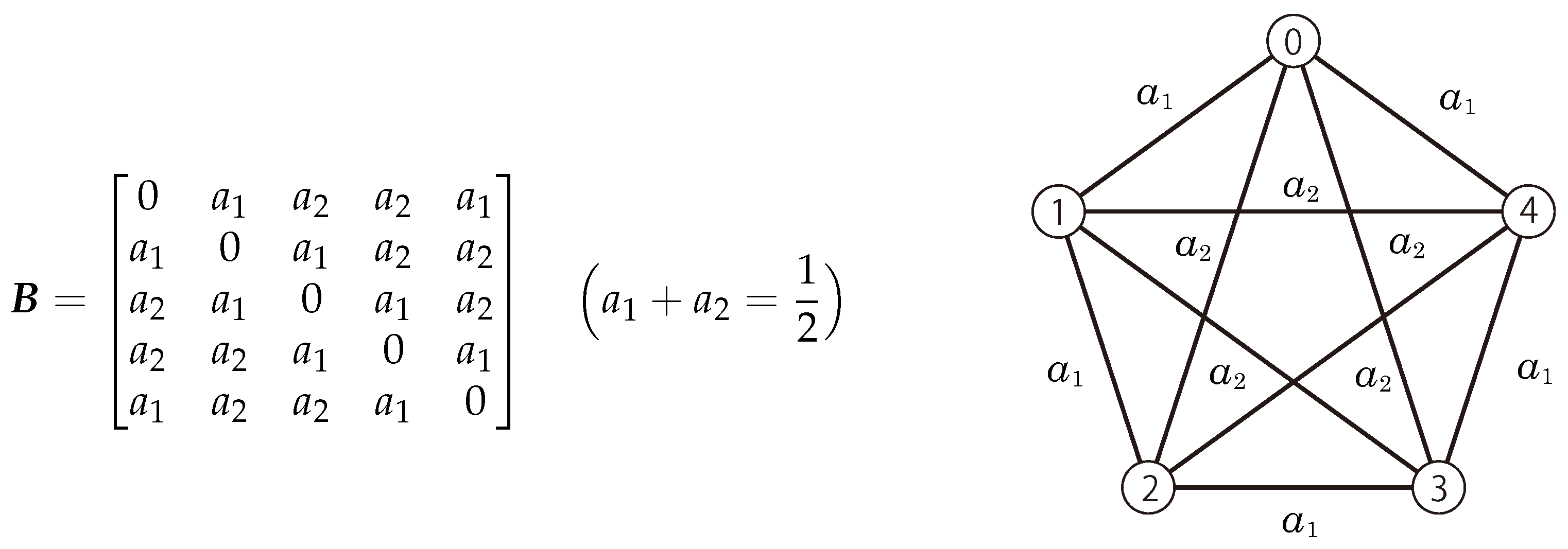
where I is the identity matrix and B is the adjacency matrix of G (see Figure 1).
Here, and:
The function is defined as .
The matrix B is a symmetric stochastic matrix, expressed as follows [10]:
where:
A can also be expressed in terms of the permutation matrix as follows:
The following proposition is a direct consequence of A defined in (3).
Proposition 1.
Let with a vertex set, . Subsequently, the generalized graph Laplacian A on G has the following eigenvalues:
():
():
From Proposition 1, all eigenvalues are distributed as follows:
Let be the characteristic polynomial for A:
where:
3. Discrete Sobolev Inequalities
Let be the weighted complete graph in Definition 1. For each vertex , we attach a complex number, . For the vector , we define two types of Sobolev energies (i.e., potential energies) using the generalized graph Laplacian:
where a is a positive dumping constant.
To explain our conclusion, we assume that and that is a Penrose–Moore generalized inverse of A. In particular, satisfies:
is the orthogonal projection matrix to the eigenspace corresponding to the eigenvalue of A. Hereafter, we refer to as the pseudo-Green matrix.
To prove the relation (4), we derive spectral decompositions of and . Since the generalized graph Laplacian A is an real symmetric matrix, A is diagonalized as using the unitary matrix . Vectors are eigenvectors corresponding to eigenvalues of A. Furthermore, vectors are chosen such that they satisfy the relation , where is the Kronecker delta. The orthogonal projection matrices defined by satisfy:
Using the projection matrices, the generalized graph Laplacian A and the identity matrix I have the following symmetric eigenvalue decompositions:
Thus, we have:
From the above discussions, the spectral decompositions of and are expressed as follows:
Thus, we arrive at the following theorems.
Theorem 1.
Let and . For any , there exists a positive constant C, independent of u, such that the discrete Sobolev inequality:
holds. Among the set of Cs, the sharp constant is expressed as follows:
If C in the above inequality is replaced by , the inequality becomes an equality for any column vector u of .
Theorem 2.
Let and . For any satisfying , there exists a positive constant C that is independent of u, such that the discrete Sobolev inequality:
holds. Among the set of Cs, the sharp constant is expressed as follows:
If C is replaced by in the above inequality, the equality holds for any column vector u of .
We now explain the physical meaning of Theorems 1 and 2. A real-valued represents a deviation from the steady state. In each discrete Sobolev inequality, the square of the maximum deviation is estimated by a constant multiple of the potential energy, or . Hence, the sharp constant is expected to represent the rigidity of the mechanical model corresponding to the weighted complete graph.
From (11), it follows that is a monotonically-decreasing function of a. From the monotonicity with respect to a, Equations (9), (11) and (13), we obtain the following theorem:
Theorem 3.
The following relation holds:
Since the proofs of the main Theorems 1–3 are essentially equivalent to those given in [11], we omit them.
4. Sharp Constants
In this section, we compute the entries on the main diagonals of the Green matrices, which are the sharp constants of the discrete Sobolev inequalities.
For , we introduce the j-th unit vector as:
which is essential for deriving our conclusion.
Proposition 2.
For any , we have:
can also be expressed in terms of the expansion coefficients of the characteristic polynomial as follows:
Proof of Proposition 2.
As G is a Toeplitz matrix, for any , we obtain:
Here, we have used Equation (7). Furthermore, after reducing this expression to a common denominator, we obtain the following expression using the expansion coefficients of the characteristic polynomial:
The proof of Proposition 2 is now complete. ☐
Proposition 3.
For any , we have:
can also be expressed in terms of the expansion coefficients of the characteristic polynomial as follows:
Proof of Proposition 3.
Since is a Toeplitz matrix, for any , we therefore obtain:
Here, we have used Equation (8). Again reducing to a common denominator, we obtain the following expressions using the expansion coefficients of the characteristic polynomial:
():
():
The proof of Proposition 3 is now complete. ☐
5. Conclusions
In this section, we prove that the sharp constants and satisfy certain hierarchical structures.
For , we define the elementary symmetric polynomials on n variables as follows:
We also define the following special value in the elementary symmetric polynomial.
Note that is positive. The constants satisfy the following lemmas.
Lemma 1.
For , we have the following inversion formulae:
- (i)
- (ii)
Proof of Lemma 1.
(i) For , we introduce the following matrices:
where:
The constants and satisfy the following equality:
From the above equality, we have:
Thus, we have:
(ii) Since the inverse matrix of is given by:
where:
we have:
The Proof of Lemma 1 is now complete. ☐
Lemma 2.
For , we have:
Proof of Lemma 2.
From Lemma 1, we have:
The Proof of Lemma 2 is now complete. ☐
We first show that the sharp constants satisfy a hierarchical structure.
Theorem 4.
For , if:
the sharp constants satisfy the following hierarchical structure:
Proof of Theorem 4.
Taking the difference between and , the determinant formula is obtained as:
From the assumption, we obtain:
From the above inequality, the sharp constant is a monotonically-decreasing sequence with respect to n. Paying attention to the equality:
we have obtained the hierarchical structure for the sharp constants .
The proof of Theorem 4 is now complete. ☐
By using the elementary symmetric polynomials (16), we also define the following special value.
Note that is positive.
The following theorem shows that the sharp constants satisfy a hierarchical structure.
Theorem 5.
For , if:
the sharp constants satisfy the following hierarchical structure:
Proof of Theorem 5.
Taking the difference between and , we obtain the determinant formula:
From the assumption, we obtain:
According to the above inequality, the sharp constant is a monotonically-increasing sequence with respect to n. Focusing on the equality:
we obtain the following hierarchical structure for the sharp constants .
The proof of Theorem 5 is now complete. ☐
6. Examples
6.1. Example 1 (See [8])
Let G be a weighted complete graph, , with a vertex set, . We define the adjacency matrix as follows:
Subsequently, for , the generalized graph Laplacian A on G is given by:
We obtain the following theorem from Theorems 4 and 5.
Theorem 6.
For , the sharp constants hold the following hierarchical structure:
- (i)
- ,
- (ii)
- .
The proof of Theorem 6 is simple, so we omit it. It is interesting to note that and , which are related by Theorem 3, satisfy opposite hierarchical structures.
6.2. Example 2
Let G be a weighted complete graph, , with a vertex set, . We define the adjacency matrix as follows:
Subsequently, for , the eigenvalues of the generalized graph Laplacian A on G are given by:
Acknowledgments
The authors K.T. and A.N. were supported by the JSPS Grant-in-Aid for Scientific Research (C) Nos. 17K05374 and 25400146.
Author Contributions
The section of conclusions is based on some ideas by K.T. All of the authors have contributed to the writing of this paper. They read and approved the manuscript.
Conflicts of Interest
The authors declare no conflict of interest.
References
- Aubin, T. Problèmes isopérimétriques et espaces de Sobolev. J. Differ. Geom. 1976, 11, 573–598. [Google Scholar] [CrossRef]
- Talenti, G. Best constant in Sobolev inequality. Ann. Mat. Pura Appl. 1976, 110, 353–372. [Google Scholar] [CrossRef]
- Kametaka, Y.; Watanabe, K.; Nagai, A. The best constant of Sobolev inequality in an n dimensional Euclidean space. Proc. Jpn. Acad. Ser. A Math. Sci. 2005, 81, 57–60. [Google Scholar] [CrossRef]
- Takemura, K.; Yamagishi, H.; Kametaka, Y.; Watanabe, K.; Nagai, A. The best constant of Sobolev inequality corresponding to a bending problem of a beam on an interval. Tsukuba J. Math. 2009, 33, 253–280. [Google Scholar] [CrossRef]
- Takemura, K.; Kametaka, Y.; Watanabe, K.; Nagai, A.; Yamagishi, H. Sobolev type inequalities of time-periodic boundary value problems for Heaviside and Thomson cables. Bound. Value Probl. 2012, 2012, 95. [Google Scholar] [CrossRef]
- Chung, F.R. Spectral Graph Theory; American Mathematical Society: Providence, RI, USA, 1997. [Google Scholar]
- Van Dal, R.; Tijssen, G.; Tuza, Z.; Van der Veen, J.A.A.; Zamfirescu, Ch.; Zamfirescu, T. Hamiltonian properties of Toeplitz graphs. Discret. Math. 1996, 159, 69–81. [Google Scholar] [CrossRef]
- Yamagishi, H.; Kametaka, Y.; Watanabe, K. The Best Constant of Three Kinds of the Discrete Sobolev Inequalities on the Complete Graph. Kodai J. Math. 2014, 37, 383–395. [Google Scholar] [CrossRef]
- Olshevsky, V.; Strang, G.; Zhlobich, P. Green’s matrices. Linear Algebra Appl. 2010, 432, 218–241. [Google Scholar] [CrossRef]
- Horn, R.A.; Johnson, C.R. Matrix Analysis, 2nd ed.; Cambridge Unversity Press: Cambridge, UK, 2013. [Google Scholar]
- Takemura, K.; Nagai, A.; Kametaka, Y. Two types of discrete Sobolev inequalities on a weighted Toeplitz graph. Linear Algebra Appl. 2016, 507, 344–355. [Google Scholar] [CrossRef]
Figure 1.
Symmetric adjacency matrix B of a weighted complete graph, .

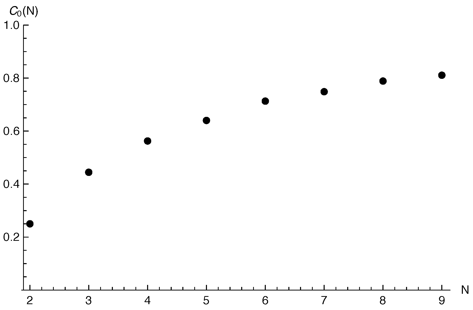
Figure 2.
.

Figure 3.
.

© 2017 by the authors. Licensee MDPI, Basel, Switzerland. This article is an open access article distributed under the terms and conditions of the Creative Commons Attribution (CC BY) license (http://creativecommons.org/licenses/by/4.0/).
Share and Cite
MDPI and ACS Style
Takemura, K.; Kametaka, Y.; Nagai, A. A Hierarchical Structure for the Sharp Constants of Discrete Sobolev Inequalities on a Weighted Complete Graph. Symmetry 2018, 10, 1. https://doi.org/10.3390/sym10010001
AMA Style
Takemura K, Kametaka Y, Nagai A. A Hierarchical Structure for the Sharp Constants of Discrete Sobolev Inequalities on a Weighted Complete Graph. Symmetry. 2018; 10(1):1. https://doi.org/10.3390/sym10010001
Chicago/Turabian StyleTakemura, Kazuo, Yoshinori Kametaka, and Atsushi Nagai. 2018. "A Hierarchical Structure for the Sharp Constants of Discrete Sobolev Inequalities on a Weighted Complete Graph" Symmetry 10, no. 1: 1. https://doi.org/10.3390/sym10010001
Note that from the first issue of 2016, this journal uses article numbers instead of page numbers. See further details here.