Abstract
This paper deals with a method for removing a ghost target that is not a real object from the output of a multiple object-tracking algorithm. This method uses an artificial neural network (multilayer perceptron) and introduces a structure, learning, verification, and evaluation method for the artificial neural network. The implemented system was tested at an intersection in a city center. Results from a 28-min measurement were 88% accurate when the multilayer perceptron for ghost target classification successfully detected the ghost targets, and 6.7% inaccurate when ghost targets were mistaken for actual targets. This method is expected to contribute to the advancement of intelligent transportation systems if the weaknesses revealed during the evaluation of the system are complemented and refined.
1. Introduction
Radar sensors have an indispensable role to play in autonomous vehicles, intelligent transportation systems, and robotics. Radar sensors have a lower angular resolution than sensors like lidar and cameras, but they have the advantage of detecting objects behind obstacles and determining the speed of moving objects. Sensors like radar and sonar detect ghost targets due to multipath propagation of waves. A ghost target is not an actual target, but rather a kind of illusion where the reflected wave arrives at the actual target but returns on a path that is not the shortest path [1]. Such a ghost target makes it difficult to accurately detect a vehicle, person, or other object, and decreases the reliability of the sensor by increasing the probability of false alarm. Knudde et al. employed a method called Hoegbom CLEAN, which was originally used to process radio astronomy images to remove ghost targets and to isolate real targets from other clusters. But due to its iterative property, paralleling the process in any multiprocessor architecture can be difficult [2]. Lee and Lee devised a statistical model that can be applied to rejecting ghost targets generated by multipath propagation. However, the model requires one to discriminate the indirect paths that are the origins of the ghost targets from the direct paths, which is a non-trivial process [3]. Jin et al. develop a mathematical image formation technique named time reversal TR-SAR [4]. However, the method requires one to model the exact response of a system as a new target added to the system [5]. Lin et al. used the characteristics of a triangular waveform, which is used for frequency modulated continuous wave (FMCW) radar sensors, in order to reject multipath ghost targets. Since this method is not a software post-processing method, it is difficult to flexibly cope with environmental changes [6]. Roos et al. devised a method that rejects ghost targets by designing a model that describes ghost targets, utilizing the motion state of an ego vehicle. However, in some cases, two radar sensors are required [7]. The proposed method, thanks to its non-iterative property, can be fully parallelized and accelerated by including a graphics processing unit (GPU) and a symmetric, multiprocessor architecture. As a matching learning approach, it does not require one to model the real world by hand; therefore, it can easily be fully automated. In this paper, we introduce a post-processing method using an artificial neural network that removes ghost targets and that will improve the reliability of tracking algorithms, such as radars.
2. Ghost Targets and Multiple Target Tracker
In real situations, a radar sensor produces imaginary targets (the so-called ghost targets). These have nothing in common with real objects, like vehicles or pedestrians, but are from multipath propagation of a transmitted radar wave or due to interference from other radar sensors.
Figure 1 illustrates a situation where radar signals echo from the same position through multiple paths. If the radar signal echoes from its destination to the sensor via the shortest path, there will be no problem getting information about the target, but in real situations, radar signals do not do that. Even radar signals from other radar sensors can interfere with transmitted radar signals. These are the causes of ghost targets.
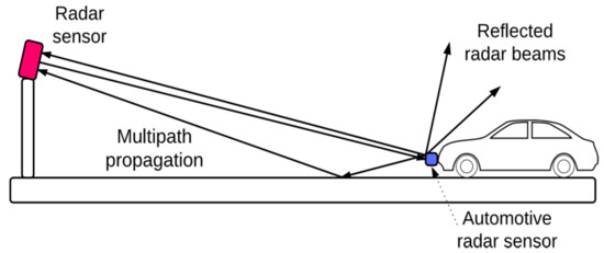
Figure 1.
Propagation of radar signals.
2.1. Characteristics of Ghost Targets
The characteristics of normal objects and ghost targets were analyzed. Features like lifetime of a track, weight β0, and longitudinal and lateral coordinate differences in velocity and position were used in the analysis.
2.1.1. Characteristics of Track Lifetime
Track lifetime indicates how many scans were processed since the measurement associated with the track first appeared. Figure 2 shows the generation-time distribution for general objects and ghost targets. Generation time of a general object is distributed between 0 and 4000 scans, while generation time of a ghost target is mainly distributed within 100 scans. This reflects ghost targets that disappear soon after they are created.
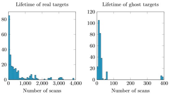
Figure 2.
Comparison of track lifetime between tracks associated with real targets and ghost targets.
2.1.2. Characteristics of Weight β0
Weight β0, an important variable for a probabilistic data association filter (PDAF), determines how much the i-th measurement in the validation gate of one tracker influences the tracker’s correction phase [8]. Each target where the location is estimated using the PDAF is determined by the measurements belonging to the target's validation gate. At this time, the degree to which each measurement value affects the estimation of the target position is the weight . This weight is also called the association probability. Weight is the i-th measurement value in the validation gate via Equations (1) and (2) [9]:
where is weight before normalization, is the number of all measurements in the validation gate, and is the probability of detection. is the gate probability (the probability that the real measurement will be included in the valid gate), and is the spatial density of a false measure that exists along a continuous uniform distribution in the measurement volume [9]. If i = 0, no measurements in the valid gate are relevant to the tracker, and only the predicted values for the previous state of the tracker are used in the correction phase.
Ghost targets are less likely to exhibit similar conditions across multiple scans; that is, inter-scan coherency is small. Therefore, if a ghost target is included in the validation gate of a tracker, then the same ghost target is less likely to be included in the validation gate in the next scan. In other words, if only one ghost target is included in the validation gate of the tracker, then there is a high probability that no measurements will be included in the next scan. The index that numerically reflects this is β0. As shown in Figure 3, if several measurements enter the validation gate in the correction step, the calculated β0 is small and close to zero. On the other hand, if no measurements are included in the validation gate, then the calculated β0 will be 1.
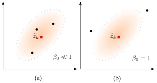
Figure 3.
Difference in weight β0 with and without measurement in the validation gate: (a) at least one measurement exists; (b) no measurements exist.
Figure 4 shows that the β0 distribution of the actual object and the ghost target have different tendencies. Most real objects have a weight close to 0, whereas most of the weight values of ghost targets are close to 1.
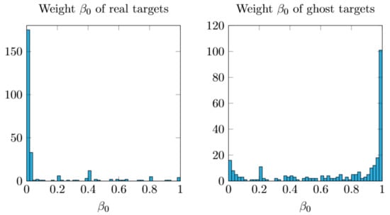
Figure 4.
Weight β0 distribution of the actual target (left) and the ghost target (right).
2.1.3. Characteristics of Displacement and Velocity
Figure 5 shows that actual objects and ghost targets have different distributions (even at the tracker’s estimated position), and Figure 6 shows the difference between the position in the previous scan and the current scan. A radar installed in a fixed position captures the movement of vehicles approaching in the longitudinal direction. Therefore, the real target generally tends to move in the longitudinal direction, and the ghost targets show no special behavior or lateral movement compared to real targets.
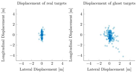
Figure 5.
Displacement distribution of actual targets (left) and ghost targets (right).
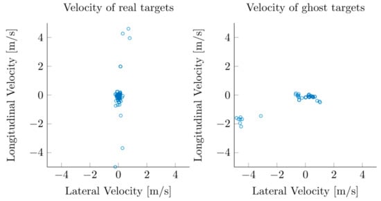
Figure 6.
Velocity distribution of actual targets (left) and ghost targets (right).
This study aims to measure the traffic volume of approaching vehicles from a straight road to a radar, so mainly longitudinal displacement is measured, and the velocity is also the same. With a ghost target, we can see that the deviation in displacement is larger in the lateral direction than in the longitudinal direction, which is the main running direction of the vehicle. We can also see that the velocity deviates more in the lateral direction than in the longitudinal direction.
2.2. Choosing the Most Suitable Classification Method
It is necessary to select a suitable classification method to classify a tracked object as either a real object or a ghost target. Considering the purpose of this study and future possibilities, we set the following criteria for selecting appropriate classification methods.
- It is important to be able to easily add classes, such as whether something is a stationary object or a moving object, instead of only distinguishing whether the object being tracked is an actual object or a ghost target;
- It should be possible to determine the degree to which the object being tracked belongs to each class (ghost or actual);
- The training time should be short.
Criterion 1 means that the tracker is currently limited to whether a classifier is used to determine if a target is a ghost or not, but future research will make it possible to distinguish between moving objects and stationary objects by subcategorizing actual objects without major modification of the classifier.
Criterion 2 means that the classification algorithm should be able to determine how much the degree of a ghost target is larger than the degree of an actual object without merely indicating whether or not the ghost target is simply displayed.
Criterion 3 is to minimize trouble with the classifier learning process (which must be frequent) because actual objects and ghost targets are different, based on the installation of the radar.
2.2.1. Comparison of Classification Methods
Implementation of this study was based on the premise that it operates on low-performance embedded devices. Therefore, the classification method used should be implemented in a native-friendly language, such as C, so it can achieve high performance. Several candidate classification methods were selected, considering this and the criteria in Section 2.2.
Table 1 shows some of the machine-learning classifiers compared with the criteria in Section 2.2 [9]. A description of the classifier according to each evaluation criterion follows.

Table 1.
Comparison of various classification methods [10].
- A support vector machine is basically a binary classifier that can determine only two classes. Although it is known that extensions can be made to differentiate several classes [11], the application of this method requires a significant amount of modification. A multilayer perceptron can easily be expanded by simply adding as many output nodes as the number of newly added classes. A decision tree is also easily expanded by relearning or by adding a new class label pair to the training set.
- The output of a support vector machine and a decision tree is the class label. On the other hand, a multilayer perceptron sets different labels for each output node, and then inputs the characteristics of the training data into each input node, one by one. Then, the multilayer perceptron sets the value of the output node corresponding to the correct label to 1, and sets the rest to 0, or any small value. The values of each output node for the data to be predicted by the multilayer perceptron (after all the training processes) have a real range. The larger the value, the more likely it is to belong to that class. Since a multilayer perceptron has this characteristic, it is easy to determine through the value of the output node corresponding to each class whether the prediction results of certain data are more likely to belong to one class than to another class.
- A support vector machine and a multilayer perceptron have longer learning times than a decision tree. However, the multilayer perceptron has room to shorten the learning time by adjusting the number of middle layers and the number of nodes in each layer.
The classifier selected after considering these three criteria was the multilayer perceptron. A multilayer perceptron can determine how much higher the likelihood is that the data to be classified belong to one class, compared to how much they belong to another class, and the degree of comparison can be evaluated. In addition, the number of intermediate layers and the number of nodes in each layer can be adjusted appropriately, according to the application environment, thereby shortening the learning time.
2.2.2. Target Classification Using a Multilayer Perceptron
In order to find actual objects and ghost targets of the tracked objects with the six characteristics of generation time, weight, vertical and horizontal displacement, and longitudinal and transverse velocity, this study selected the multilayer perceptron as the learning algorithm. These six features are input into each node of the input layer. The output layer has two nodes, O1 and O2, which represent real objects and ghost targets, respectively.
In other words, the learning of actual objects should be such that the values of the output nodes are O1 = 1 and O2 = 0, and learning ghost targets returns O1 = 0 and O2 = 1. The specific settings and details of the multilayer perceptron used are described in Section 3.2.3.
2.3. Multiple Target Trackers
This study used a PDAF for multiple-target tracking. The devised multiple-target tracker, which is based on the PDAF, labels each track with four states: undefined, candidate, confirmed, and coasting as shown in Figure 7 [8]. Undefined is assigned to targets that had never been processed before. If a track keeps a candidate state for a predefined number of ticks, then it becomes confirmed. The confirmed state is assigned to the tracks that need to be displayed. A confirmed track transforms into a coasting track if no measurement is associated for a predefined number of ticks. The devised multiple-target tracker consists of five procedures. These procedures execute sequentially but can be pipelined if needed.
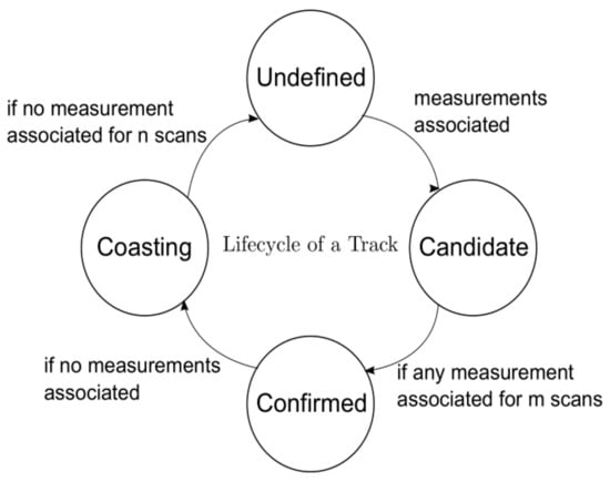
Figure 7.
Lifecycle of a track.
2.3.1. Track Management Procedures
For each tick, a set of measurements is read by the radar sensor as shown in Figure 8 (Read radar detections, Figure 8). If a measurement is close enough to a track, it is used to update the state of the track. If not, the measurement itself becomes a track. Tracks that have no associated measurement for a predefined number of ticks are deleted by the tracker (Associate measurements and Update tracks, Figure 8).
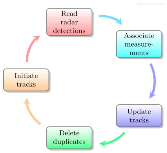
Figure 8.
Five procedures of the devised multiple target tracker.
Algorithm 1 depicts the detailed track-updating process, where x is the state of a track, and z is the state of a measurement. F, P, H, K, and S are state transition matrix, covariance matrix, measurement space to state space conversion matrix, Kalman gain, and predicted measurement covariance from the PDAF, respectively; variables with a bar are predicted counterparts of each variable, and variables with no specific definition are temporary placeholders. The update tracks stage modifies each track’s state (which uses measurements that have been assigned) and iterates all the tracks currently managed by the tracker. At first, the procedure makes each track’s state transit as described in Section 1. Then, it predicts each track with a Kalman filter. If no measurements are assigned to the track, predicted measurement z is inserted into its measurement list. Auxiliary variable sum, which is needed to accumulate weight β, is calculated. Then the actual track state update is followed, and the last state of the track is kept for deleting duplicates. The duplication deletion stage simply deletes two tracks where histories are the same. Dissimilarity used for deletion is the Euclidean distance between two tracks. If dissimilarity between two tracks is below a set threshold, then one of them will be deleted (Delete duplicates, Figure 8).
| Algorithm 1. Track update procedure. |
| Procedure UpdateTracks(measurement measurements[·]) |
| for all t in Trackers[·] do |
| DoTransition(t) |
| x = t.F * t.x |
| P = t.F * t.P * t.FT + t.Q |
| z = t.H * x |
| S = t.H * P * t.HT |
| K = P * t.H * S−1 |
| Pc = (I − K * H) * P |
| if t.measurementNumber == 0 then |
| insert z into t’s measurement list |
| end if |
| sum = 0 |
| for every measurement m in t’s measurement list do |
| m.ν = m.z − z |
| m.L = exp[−1/2m.νT * S−1 * m.ν] |
| sum = sum + m.L |
| end for |
| L = 8 * (1 − PG * PD) * t.measurementNumber/PD*γ2 |
| sum = sum + L |
| for every measurement m in t’s measurement list do |
| m.β = m.β/sum |
| P = P + m.β * m.ν * m.νT |
| νc = m.ν * m.ν |
| end for |
| P = K * (P − ν * vT) * KT |
| t.P = L * P + (1 − L) * Pc + P |
| t.x = x + K * νc |
| add t.x into t’s history list |
| add L into t’s β0 list |
| end for |
| end procedure |
2.3.2. Dynamic System Model
This study used a PDAF for multiple-target tracking. Assume that the motion of each target is a constant velocity model. The constant velocity model is as follows:
where , are the position coordinates of the x, y axes at time k − 1 of the object, and , are velocity. is the noise that follows . Since the interval of each discrete time is as short as 66 ms, the vehicle speed difference is negligibly small. For this reason, a constant velocity model was used.
The parameters used in this study are as follows:
Mapping matrix uses the identity matrix (I), because the measurement space and state space are the same; initial covariance for initializing the tracker also uses identity matrix I. In the PDAF, the number of tracks = 40, the probability of a validated gate is , the probability of detection is , the threshold of validated gate , candidate steps = 5, and coast steps = 6. These values were determined through trial and error.
3. Implementation and Evaluation
This section introduces the hardware and software configurations used to implement a multi-object tracker, and discusses the performance evaluation of the implemented results.
3.1. Implementation
3.1.1. Radar Sensor
The sensor used in this study is Continental’s ARS-308 long-range radar sensor. The sensor ensures the relative position and velocity of the object with respect to the radar sensor’s position using the FMCW waveform in the 77 GHz band.
Table 2 shows the specifications of the ARS-308. From up to 200 m away, it is possible to detect objects up to 4.3 degrees above and 28 degrees to the left and right in the direction in which the sensor points. The distance resolution means that two objects are separated by at least 2 m, and the speed difference is more than 5.5 km/h. Angular resolution means that, like distance resolution, when two objects are at a distance, they are separated by one degree, and when they are close to each other, by two degrees.
Table 2.
Technical specifications of the ARS-308 radar sensor.
The ARS-308 outputs a list of measurements every 66 ms. The maximum number of measurements that can be included in one scan is 128. Communication with the outside uses a controller area network (CAN), which is widely used as a network protocol inside a vehicle.
3.1.2. Software
A linear algebra library, Eigen, was used to quickly process frequent matrix operations. Eigen has fast speed and high reliability. It is used for the Large Hadron Collider of the European Nuclear Research Center. Also used was the MATLAB matrix operation software and a robot operating system.
3.1.3. Graphical User Interface
Figure 9 shows the user interface of this study’s implementation for easy tracking of multiple objects in real time. The user interface uses Qt, which is widely used as a cross-platform application framework. The status of the tracker is represented by a blue square point, along with the top tracker identification number, speed, and the position of each measurement, indicated by a gray rounded dot. The lanes are represented by dotted lines in the longitudinal direction, and the number of lanes and the width of each of the lanes can be instantly modified through a menu on the user interface. In order to cope with cases where the installation angle of the radar does not match the direction of the road, a function to rotate the radar measurements with respect to the origin is implemented.
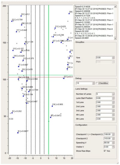
Figure 9.
Graphical user interface of the implemented program.
Considering the potential applications of this implementation (speed-trap cameras), the following points were taken into account. When the object being tracked passes through a specific point on the road, the lane number and velocity for the position of the object are recorded. This specific point can be adjusted using the user interface, and the changes are immediately reflected in the modification.
3.2. Evaluation
In this section, we evaluate the performance of the implemented radar traffic measurement system by using the multiple-object tracker (designed from the aspect of a practical application), and we quantitatively examine the ghost target discrimination ability of the artificial neural network constructed to remove ghost targets.
3.2.1. Measurement Environment
The measurements were carried out at the overpass of the Nakseom intersection in Yonghyun 5 Dong, Nam-gu, Incheon, located within 1 km of the Nakseom intersection with a starting point at the Kyungin Expressway and an ending point at the origin of the 2nd Kyungin Expressway. The radar traffic measurement system was installed at a pedestrian crossing across the southwest road of the Nakseom intersection, and was installed along the road to the southwest. The arrow in Figure 10 shows the location of the Nakseom intersection, and the translucent red triangle shows the field of view of the radar traffic measurement system (see Figure 11). The vehicles measured are those coming in the direction opposite to the radar direction.
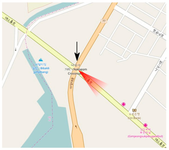
Figure 10.
Measurement environment of the implemented system.
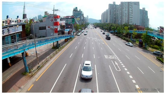
Figure 11.
Field of view of the implemented system.
3.2.2. Traffic Measurement Results
We counted the traffic volume in each lane four times for five minutes. The results are shown in Table 3. Parentheses indicate relative errors. The max relative error was 22%, and the average traffic volume error was 19%. In the second stage, which showed an average error of 19%, it was found that there were many vehicles waiting for a red signal. Because of this, it is difficult to distinguish the radar from the longitudinal resolution of the radar because of the narrow distance between cars, and it appears that multipath propagation is not canceled due to the narrow distance from an adjacent vehicle, but is introduced into the radar.
Table 3.
Traffic measurement results.
3.2.3. Configuration of the Multilayer Perceptron
An artificial neural network framework, Keras, was used to implement the multilayer perceptron. Keras features highly accessible modules, because it is implemented in Python.
Figure 12 represents the structure of a multilayer perceptron for separating ghost targets from real targets. The input layer (dense input 23) has six elements, which are tracker generation time, weight β0, longitudinal displacement and velocity, and lateral displacement and velocity. The input data pass through a fully connected layer using a rectified linear unit (ReLU) as its active function. At this point, some of the nodes in the layer are dropped. Dropout is one of the normalization methods that perform learning by randomly selecting and removing some nodes in one layer of the artificial neural network, and it is possible to achieve high accuracy by preventing models from overfitting [12,13]. The hidden layer data pass to the output layer where some ReLU nodes are dropped through a connection using softmax as an active function to form two output nodes (dense 69): (a) a ghost target; and (b) not a ghost target.
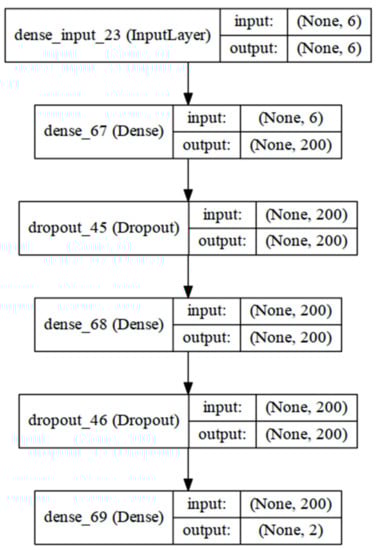
Figure 12.
Structure of the multilayer perceptron for distinguishing ghost targets.
3.2.4. Training Method of the Multilayer Perceptron
The features we used to detect ghost targets include lifetime of a track, weight β0, and longitudinal and lateral coordinate differences in velocity and position.
Since the number of data sets that can be used is no more than 540, leave-one-out-cross-validation (LOOCV) was used in order to use both the training data and the test data. LOOCV is an extreme version of k-fold crossover validation, in which only one of the data sets is set as a test data set so that all the data are test data at once. LOOCV is one of the methods used to prevent overfitting in small data sets and to evaluate them [14].
To prevent overfitting, we used 10% of the training data set as a validation data set. And the training was stopped if the loss function does not improve by repeating the epoch.
3.2.5. Evaluation of the Classifier Accuracy
Table 4 represents the confusion matrix of the multilayer perceptron for the removal of ghost targets. We can see from the table that 43.2% of the actual targets are correctly classified as targets, and 45.3% are properly classified as ghost targets, with 5.5% of the actual targets judged to be a ghost target, and 6.0% of the ghost targets mistaken as actual targets.
Table 4.
Confusion matrix of ghost targets and real targets classified by the multilayer perceptron.
As a result of the experiment, accuracy is 88.43% and recall is 88.62%. However, the false positive rate is 11.74%, which was slightly higher. This means that 11.4% of the actual targets (16,168/142,020) were removed by mistaking them for ghost targets, and 11.1% of the ghost targets (17,562/149,580) were mistaken for actual targets. In view of the fact that the multilayer perceptron designed in this study is intended to pick out and quickly remove ghost targets from among trackers in the candidate state, this classifier works effectively for the removal of actual ghost targets However, it is also possible to remove an actual target, so it is necessary to adjust the algorithm to remove only ghost targets.
4. Conclusions
This paper presents a method to remove ghost targets from the results of a tracking algorithm using a radar sensor. This method determines the possibility of ghost target removal by classifying ghost targets and actual targets via learning with a multilayer perceptron. From evaluation of the system, room for improvement was found, as described below.
- To remove a ghost target, the ghost target and the actual target were found in the output of the traffic measurement system and labeled, and the multilayer perceptron was trained using LOOCV. As a result, the probability of incorrectly removing an actual target as a ghost target was 5.5%. Therefore, it is necessary to improve the neural network model more precisely so as to not misjudge actual targets as ghost targets.
- The ghost target classifier using the proposed multilayer perceptron is merely a study of the possibility of using the classification result, but it is not modified to be integrated into an actual traffic measurement system. Future work includes using C to integrate modules for removing ghost targets in order to eliminate real-time ghost targets.
It is expected that if an obstacle-recognition system or a traffic-measurement system for an autonomous driving vehicle is produced by reflecting such improvements, a system in which the maintenance effort is drastically reduced can be realized.
Acknowledgments
This work was supported by an INHA UNIVERSITY Research Grant.
Author Contributions
Inhwan Ryu and Jangwoo Kwon provided the main idea for this paper, designed the overall architecture of the proposed algorithm and wrote the paper. Inhwan Ryu and Insu Won conducted the test data collection and designed the experiment, and Insu Won and Jangwoo Kwon supervised the work and revised the paper.
Conflicts of Interest
The authors declare no conflict of interest.
References
- Smith, G.E.; Mobasseri, B.G. Analysis and exploitation of multipath ghosts in radar target image classification. IEEE Trans. Image Process. 2014, 23, 1581–1592. [Google Scholar] [CrossRef] [PubMed]
- Knudde, N.; Vandersmissen, B.; Parashar, K.; Couckuyt, I.; Javaland, A.; Bourdoux, A.; Neve, W.D.; Dhaene, T. Indoor tracking of multiple persons with a 77 GHz MIMO FMCW radar. In Proceedings of the 14th European Radar Conference, Nuernberg, Germany, 11–13 October 2017; pp. 61–64. Available online: https://biblio.ugent.be/publication/8537104/file/8537106.pdf (accessed on 3 May 2016).
- Lee, M.; Lee, J.Y. Statistical Modeling of Indirect Paths for UWB Sensors in an Indoor Environment. Sensors 2016, 17, 43. [Google Scholar] [CrossRef] [PubMed]
- Jin, Y.; Moura, J.M.; O’donoughue, N.; Mulford, M.T.; Samuel, A.A. Time reversal synthetic aperture radar imaging in multipath. In Proceedings of the Asilomar Conference on Signals, Systems and Computers, Pacific Grove, CA, USA, 4–7 November 2017; pp. 1812–1816. Available online: http://ieeexplore.ieee.org/document/4487547/ (accessed on 1 May 2016).
- O’Donoughue, N.; Moura, J.M.; Jin, Y. Signal-domain registration for change detection in Time-Reversal SAR. In Proceedings of the 42nd Asilomar Conference on Signals, Systems, and Computers, Pacific Grove, CA, USA, 26–29 October 2008; pp. 505–509. Available online: http://ieeexplore.ieee.org/document/5074456 (accessed on 3 May 2016).
- Lin, J.J.; Li, Y.P.; Hsu, W.C.; Lee, T.S. Design of an FMCW radar baseband signal processing system for automotive application. SpringerPlus 2016, 5, 42. [Google Scholar] [CrossRef] [PubMed]
- Roos, F.; Sadeghi, M.; Bechter, J.; Appenrodt, N.; Dickmann, J.; Waldschmidt, C. Ghost target identification by analysis of the Doppler distribution in automotive scenarios. In Proceedings of the International Radar Symposium, Prague, Czech Republic, 28–30 June 2017; pp. 1–9. [Google Scholar] [CrossRef]
- Bar-Shalom, Y.; Willett, P.K.; Tian, X. Algorithms for tracking a single target in clutter. In Tracking and Data Fusion; YBS Publishing: Storrs, CT, USA, 2011. [Google Scholar]
- Bar-Shalom, Y.; Daum, F.; Huang, J. The probabilistic data association filter. IEEE Control Syst. 2009, 29. [Google Scholar] [CrossRef]
- How to Choose Algorithms for Microsoft Azure Machine Learning. Available online: https://docs.microsoft.com/en-us/azure/machine-learning/studio/algorithm-choice (accessed on 3 May 2016).
- Weston, J.; Watkins, C. Multi-Class Support Vector Machines; Technical Report CSD-TR-98-04; Department of Computer Science, Royal Holloway, University of London: London, UK, 1998. [Google Scholar]
- Srivastava, N.; Hinton, G.E.; Krizhevsky, A.; Sutskever, I.; Salakhutdinov, R. Dropout: A simple way to prevent neural networks from overfitting. J. Mach. Learn. Res. 2014, 15, 1929–1958. [Google Scholar]
- Heeyoul, C.; Yunhong, M. Understanding Dropout Algorithms. Available online: http://www.dbpia.co.kr/Journal/ArticleDetail/NODE06404389 (accessed on 1 May 2016).
- Moore, A.W. Cross-Validation for Detecting and Preventing Overfitting; School of Computer Science Carneigie Mellon University: Pittsburgh, PA, USA, 2001; Available online: https://pdfs.semanticscholar.org/6696/0472e44ec9866eb5570ebed45532b8ef1217.pdf (accessed on 1 May 2016).
© 2018 by the authors. Licensee MDPI, Basel, Switzerland. This article is an open access article distributed under the terms and conditions of the Creative Commons Attribution (CC BY) license (http://creativecommons.org/licenses/by/4.0/).