Multiple Criteria Decision Making and General Regression for Determining Influential Factors on S&P 500 Index Futures

Abstract

We employ the DEMATEL-based analytic network process (D-ANP) to evaluate the weight of various factors on S&P 500 index futures. The general regression method is employed to prove the result. We then employed grey relational analysis (GRA) to examine predictive power of determinants suggested by 13 experts for fluctuations in S&P 500 index futures. This study yields a number of empirical results. (1) The explanatory power of macroeconomic factors for S&P 500 index futures outperforms that of technical indicators, as found in most of previous research papers; (2) The D-ANP revealed that five core factors (US dollar index, ISM manufacturing purchasing managers’ index (PMI), interest rate, volatility index, and unemployment rate) affect fluctuations in S&P 500 index futures, of which the US dollar index is the most important; (3) A casual diagram shows that the US dollar index and interest rate have mutual effects, and the US dollar index unilaterally affects ISM manufacturing PMI, unemployment rate, and the volatility index; (4) Granger causality test results confirmed some similar results obtained via the D-ANP that the US dollar index, interest rate, and the PMI have major impacts on the S&P 500 index futures; (5) The general regression results confirmed that four of five factors selected via the D-ANP (US dollar index, interest rate, volatility index, and unemployment rate) have strong explanatory power in forecasting the rate of return on S&P 500 index futures; (6) The GRA revealed that the explanatory power of various factors selected via the D-ANP was better for S&P 500 than for Dow Jones Industrial Average (DJIA) and Nasdaq 100 index futures; (7) The explanatory power is better for S&P 500 Industrial than for S&P 500 transportation, utility, and financial index futures.

1. Introduction

Over the past two decades, international financial markets fluctuated dramatically because of the US subprime loan crisis and five European countries debt crises. To prevent shocks induced by huge volatility in stock fluctuations in the near future, investors are anxious for identifying appropriate hedging instruments. The Taiwanese government approved listings of the ETFs of S&P 500, Nasdaq, and Dow Jones industrial indexes on the Taiwan Stock Exchange since December, 2015. These listings not only connect Taiwanese stock markets with international markets, but also provide Taiwanese investors with international financial instruments.

With the closed relationship among the financial markets of various countries, this study emphasizes that, in addition to technical factors, macroeconomic factors of each country play an essential role. In fact, the trend for US stocks has strongly and continuously rebounded since the fourth quarter of 2015 to that of 2017, and the financial reports of enterprises are much better than expected, so investor prospects have changed from extreme pessimism to extreme optimism. Since a combination of Decision Making Trial and Evaluation Laboratory (DEMATEL) and analytic network process (ANP) has been widely used to solve various decision problems considering interdependencies among factors [1], we use the DEMATEL-based ANP (D-ANP) to examine impacts among factors that can affect investors trade in S&P 500 index futures. We also perform the general regression method to confirm the results obtained by the D-ANP. Furthermore, we examine the explanatory power for four major sectors of the S&P 500 index and for three major US stock index futures for various factors selected via the D-ANP. The grey relational analysis (GRA) [2] was further to evaluate S&P 500 sectors.

The study objectives are as follows: (1) to pick various key factors out of 19 factors affecting investors trading in S&P 500 index futures by 13 experts via multiple-round questionnaires; (2) to examine mutual relationships among various key factors affecting investor trading in S&P 500 index futures using Delphi and D-ANP with the Borda method; (3) to examine the causal relationship among the five factors selected by the D-ANP, then use Granger causality test and the general regression method to investigate the relationship; (4) to examine the explanatory power for four different S&P 500 index sectors using the GRA; and (5) to examine the explanatory power for three major U.S. stock indexes futures using the GRA for various factors selected via the D-ANP.

2. Literature Review

We classified previous research into two categories: (1) articles on analytic network process (ANP) and D-ANPs; and (2) research papers concerning GRA. We first review articles on ANP and D-ANPs. Since Saaty [3] proposed ANP which has been widely applied in various fields [4,5,6,7,8,9,10,11].

It is known that, it is too time-consuming if there are various criteria regarding pairwise comparisons. The DEMATEL method was then employed for solving complicated problems, and a causal diagram was used for policy-making and for exploratory, theoretical, and large-scale empirical studies. DEMATEL was also employed to solve inner dependency problems among a set of criteria [12,13]. The D-ANP was used to solve the problems with ANP due to pairwise comparisons [1,14,15,16,17,18,19,20,21].

There has been extensive research papers on GRA. Deng [22] proposed grey system theory and emphasized the stability and stabilization of a system whose state matrix is triangular. Deng [23] listed applicable fields for the GS, including agriculture, ecology, economics, meterology, seismology, environmental science, etc. The Grey system theory has been successfully used in various research fields [24,25,26,27,28,29,30,31,32,33,34,35,36,37].

3. Methodology

3.1. Delphi Method

We first selected 19 factors that might affect S&P 500 index futures from our literature review. We then used the Delphi method to identify cause-effect relationships and weights for factors affecting S&P 500 index futures.

3.1.1. Invite Qualified Experts

Gordon and Helmer [38] proposed the Delphi method which used a continuous series of questionnaires to draw out predictions from various experts in many rounds. After each round, the result was sent back to each expert to make some adjustments based on the viewpoints from other experts. Finally, the process was completed after the accomplishment of consistency, and the average score from the final round was calculated. In this study, we invited 13 experts who had been working in the relevant field for more than five years. The academic and professional background for 13 experts are presented at

Table 1. Academic and professional background for 13 experts.

No.	Expert	Degree *	Professional Institute	No.	Expert	Degree	Professional Institute
01	A	M	LITE-ON Corp.	08	H	P	Professor
02	B	B	Taiwan Stock Exchange	09	I	M	Fubon Futures
03	C	M	Taipei Fubon Bank	10	J	M	Fubon Futures
04	D	M	Cathay Bank	11	K	M	Capital Consulting
05	E	P	Professor, Xiamen Univ.	12	L	P	Fubon Futures
06	F	P	Professor	13	M	P	Fubon Futures
07	G	P	Institute for Information	-	-	-	-

* M denotes Master, B denotes Bachelor, P denotes Ph.D.

.

3.1.2. Prototypical Structure

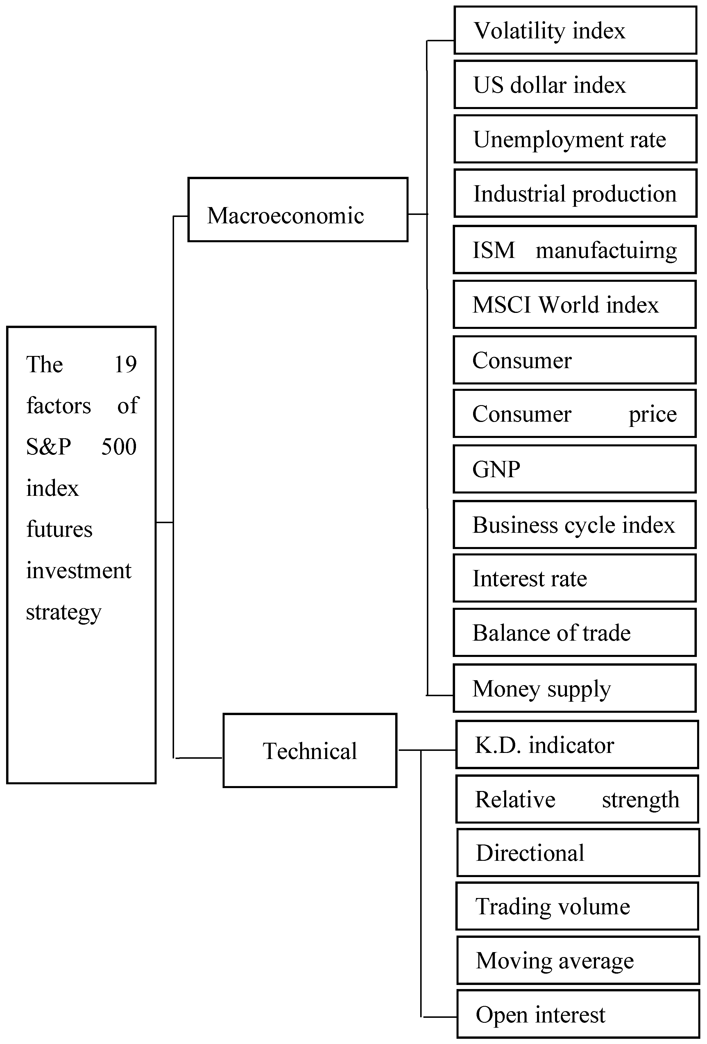
We first selected 19 factors affecting S&P 500 investment strategy from previous research papers and then used the Delphi method to interview 13 experts to develop a prototypical structure, as shown in Figure 1.

3.1.3. Amendment of the Prototypical Structure

Table 2. Amendment of the prototypical structure.

Structure	Factors	Experts’ Viewpoint	Structure	Factors	Experts’ Viewpoint
Macro-economic factors	Volatility index (VIX)	Retain	Macro-economic factors	Interest rate (IR)	Retain
	US dollar index (USDX)	Retain		Balance of trade (BOT)	Retain
	Unemployment rate (UR)	Retain		Money supply (MS)	Delete
	Industrial production index (IPI)	Retain	Technical factors	KD indicator (KD)	Retain
	ISM Manufacturing purchasing managers’ index (PMI)	Retain		Relative strength index (RSI)	Delete
	MSCI world index (MSCI)	Delete		Directional movement index (DMI)	Retain
	Consumer confidence index(CCI)	Delete		Trading volume (TV)	Retain
	Consumer price index (CPI)	Retain		Moving average (MA)	Retain
	GNP	Delete		Open interest (OI)	Retain
	Business cycle index (BCI)	Delete	-	-	-

shows how the prototypical structure was amended using the responses of 13 experts to the prototypical structure. Six factors with a weak relationship with the research subject were deleted.

3.1.4. Results for the First-Round Questionnaire

According to the amended prototypical structure, we developed a first-round questionnaire and asked 13 experts to rank each factor using a score ranging from 0 to 100. To examine the consistency among the experts, we used the consensus deviation index (CDI) to check the accuracy and set the threshold to 0.1.

Table 3. The scores of importance for the first-round questionnaire.

Structure	Factors	E1	E2	E3	E4	E5	E6	E7	E8	E9	E10	E11	E12	E13	Mean	Std. Dev.	CDI
Macro-economic factors	A4	60	65	60	65	65	65	60	70	75	65	60	75	70	65.77	5.34	0.08
	A1	80	90	80	80	80	80	80	80	85	80	90	60	80	80.38	7.21	0.09
	A2	70	70	65	70	70	60	70	70	60	75	75	65	85	69.62	6.60	0.09
	A7	60	80	85	80	85	80	75	80	80	80	85	60	85	78.08	8.55	0.11
	A3	80	85	70	80	85	60	60	80	85	80	60	80	80	75.77	9.76	0.13
	A5	85	80	60	80	80	75	60	85	85	75	60	80	80	75.77	9.54	0.13
	A6	85	65	60	65	85	65	60	65	75	60	60	65	65	67.31	8.81	0.13
	A8	65	45	50	45	50	65	45	50	45	50	45	60	50	51.15	7.40	0.14
Technical factors	B1	60	65	60	65	70	65	60	65	60	70	70	70	60	64.62	4.31	0.07
	B2	60	60	55	60	65	55	60	70	60	70	60	55	60	60.77	4.94	0.08
	B3	80	75	80	75	85	80	85	85	60	80	85	60	85	78.08	8.79	0.11
	B4	80	85	85	80	85	80	85	85	80	75	60	80	60	78.46	8.75	0.11
	B5	85	85	85	80	85	85	85	85	60	80	60	80	85	80.00	9.13	0.11

shows the average CDI score and standard deviation for the first-round questionnaire.

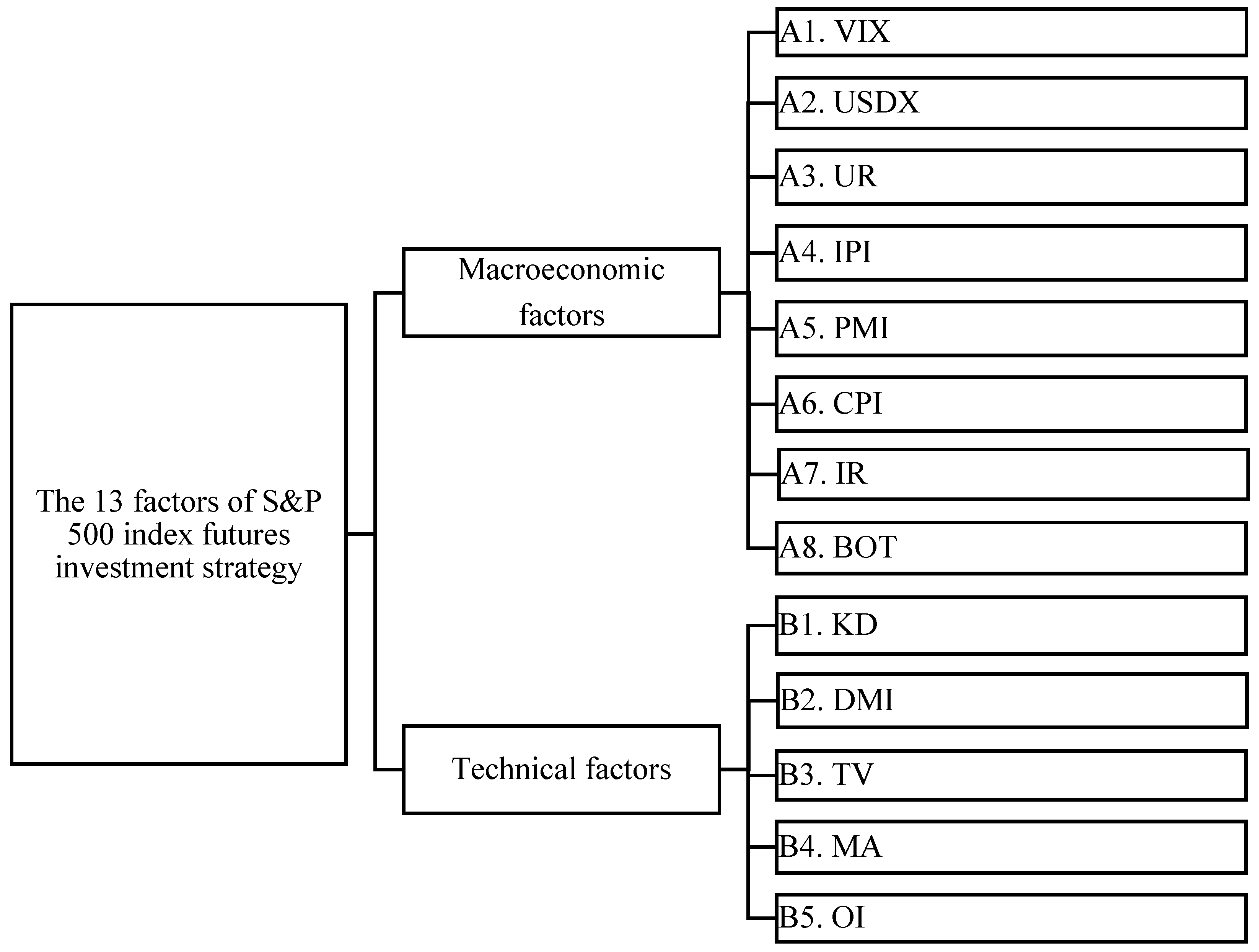
Figure 2 shows the amendment of the prototypical structure according to the suggestions of 13 experts.

3.1.5. Results for the Second-Round Questionnaire

Table 3 indicates that the CDI was >0.1 for eight of 13 factors, suggesting that the 13 experts did not have a consensus viewpoint for the first-round questionnaire. Therefore, we conducted a second-round questionnaire asking the experts to revise their first answers. The findings are presented at

Table 4. Importance scores for second-round questionnaire.

Structure	Factors	E1	E2	E3	E4	E5	E6	E7	E8	E9	E10	E11	E12	E13	Mean	Std, Dev.	CDI
Macro-economic factors	A5	85	80	80	80	80	75	80	85	85	75	80	80	80	80.38	3.20	0.04
	A7	80	80	85	80	85	80	75	80	80	80	85	80	85	81.15	3.00	0.04
	A3	80	85	70	80	85	80	80	80	85	80	80	80	80	80.38	3.80	0.05
	A6	65	65	60	65	65	65	60	65	75	60	60	65	65	64.23	4.00	0.06
	A4	60	65	60	65	65	65	60	70	75	65	60	75	70	65.77	5.34	0.08
	A1	80	90	80	80	80	80	80	80	85	80	90	60	80	80.38	7.21	0.09
	A2	70	70	65	70	70	60	70	70	60	75	75	65	85	69.62	6.60	0.09
	A8	50	45	50	45	50	50	45	50	45	50	45	60	50	48.85	4.16	0.09
Technical factors	B5	85	85	85	80	85	85	85	85	80	80	80	80	85	83.08	2.53	0.03
	B1	60	65	60	65	70	65	60	65	60	70	70	70	60	64.62	4.31	0.07
	B4	80	85	85	80	85	80	85	85	80	75	80	80	80	81.54	3.15	0.04
	B2	60	60	55	60	65	55	60	70	60	70	60	55	60	60.77	4.94	0.08
	B3	80	75	80	75	85	80	85	85	60	80	85	85	85	80.00	7.07	0.09

.

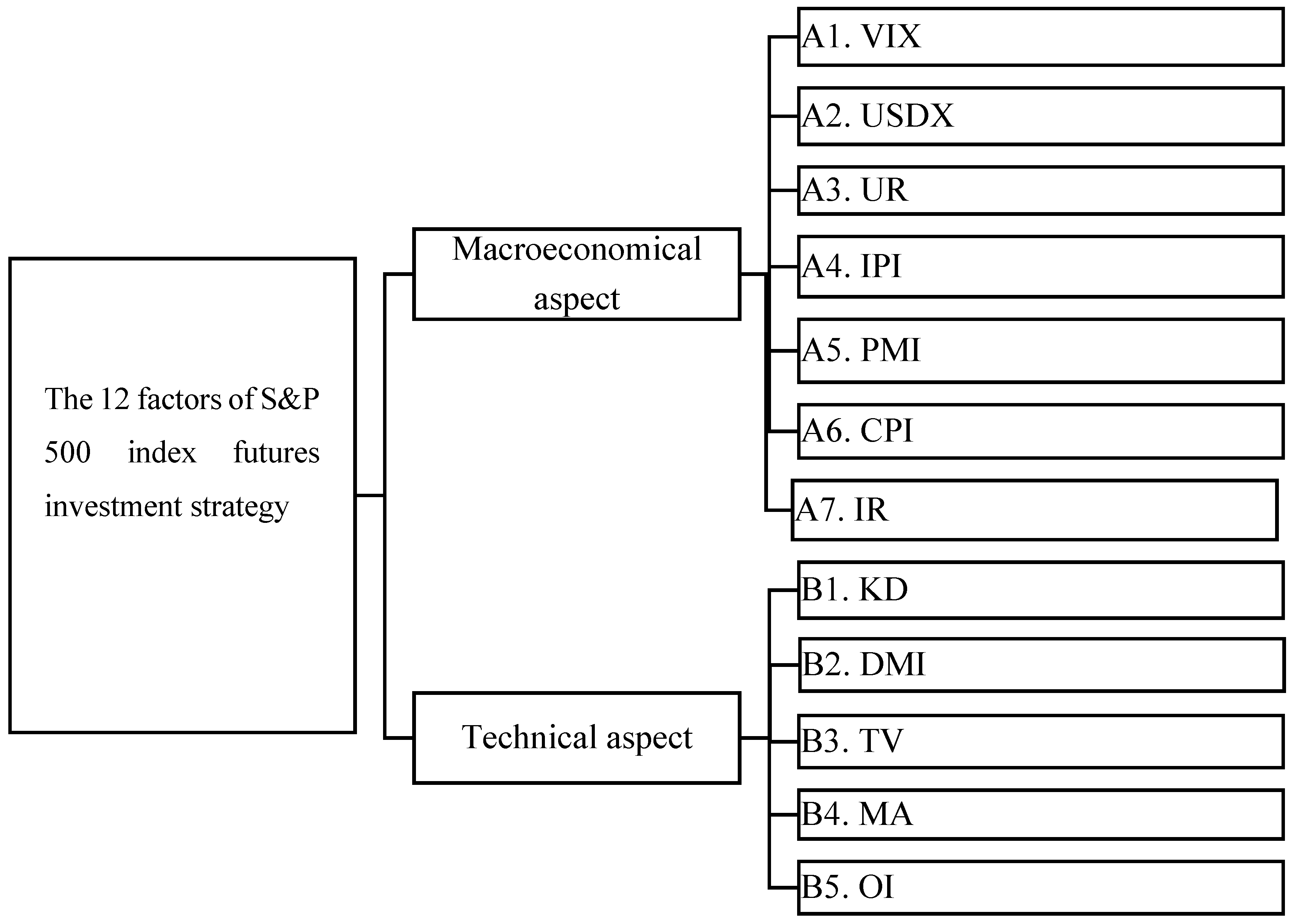
Table 4 indicates that, after the second-round questionnaire, the CDI was <0.1 for all 13 factors, suggesting that all 13 experts have consensus opinions on the second-round questionnaire. We then rearranged the order according to the average score given by the experts. Since all the experts agreed that an average score of 50 was the threshold, we deleted factor A8 as its mean score was only 48.85. Figure 3 shows the final 12 factors retained in the formal research structure.

3.2. D-ANP

The ANP employs pairwise comparisons to judge the weights for the factors of the structure and rank the possible choices in the decision. The ANP consists of the following four major stages [3,39].

• Stage 1: Model formation and problem arrangement;
• Stage 2: Pairwise comparison matrices and preference vectors;
• Stage 3: Supermatrix formulation;
• Stage 4: Select the best possible choices.

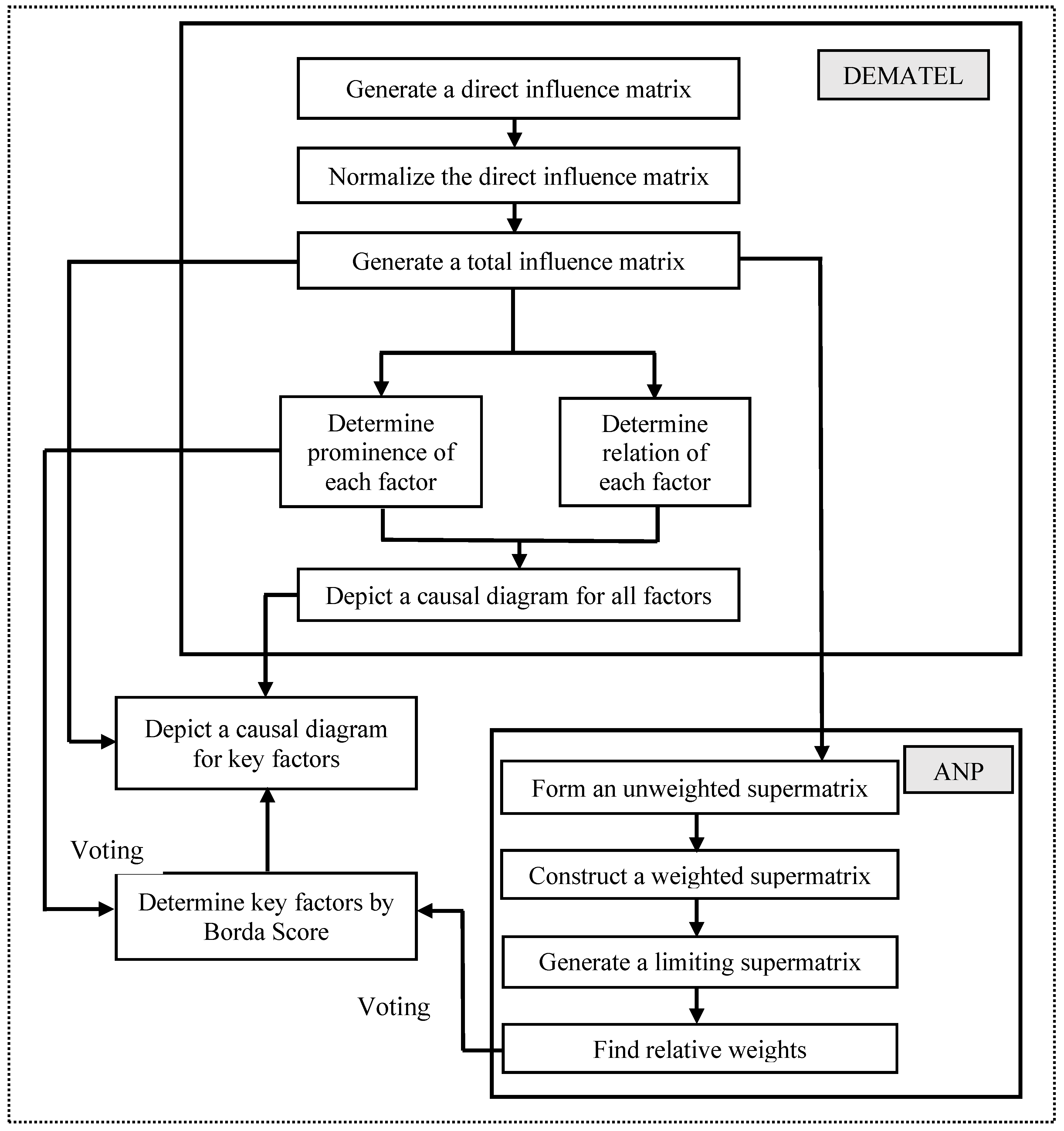
The advantage of the D-ANP is that it took the total influence matrix generated by DEMATEL as the unweighted supermatrix of ANP directly to avoid troublesome pairwise comparisons [1,19]. The flowchart of the D-ANP is depicted in Figure 4 [17]. The detail of this flowchart can be referred to [17]. In the present study, 13 experts were asked to rank the order of various factors, based on the importance of each factor, using the DEMATEL.

3.3. GRA

GRA is a useful method for evaluating alternatives. Situations for which information is lacking or incomplete are described as being grey. We used GRA to handle similar degree of complicated relations. The main idea of GRA is to obtain a grey relational grade (GRG), which can be used to explain the relationship among relevant factors. The major purpose of GRA is to measure the GRG among factors, so that the crucial rules influencing the development of the system can be found; then, the major performance characteristics of the research target can be grasped [23]. To choose the multiple alternatives, every alternative is arranged through data sequence. Any two series have a certain degree of relations [2].

GRA consists of five stages to evaluate multiple choices [24,36]:

(1)

Prepare factor compatibility;

(2)

Define data series, including reference sequences;

(3)

Calculate the grey relational coefficient (GRC);

(4)

Determine the GRG; and

(5)

Construct the grey relational order (GRD) according to GRA size.

We used GRA to analyze reference and comparative sequences to examine mutual relationship among factors. GRA treats the reference sequence as the goal to achieve, and examines the extent to which the comparative sequence approaches the reference sequence. GRA is an influence assessment model that measures the extent of likeness or unlikeness between two sequences based on the GRG. GRA allows comprehensive comparison between two sets of data rather than partial comparison by determining the length between two points. To retain this strength, all the criteria are assigned to a single level to the decision theorem. GRA was not required to find the best solution, but provides the methods for obtaining right answers for real world problems.

In present study, once the factors were identified by the 13 experts, we measured their performance for four major S&P 500 sectors: (1) industrial; (2) transportation; (3) utility; and (4) financial. We also measured the performance of three major US stock indexes (S&P 500, Nasdaq 100, and DJIA). Evaluations of the four sectors and three US stock indexes were treated as grey system problems because the information is incomplete.

3.4. Econmetrical Model

3.4.1. ADF Test

We used an augmented Dickey-Fuller (ADF) model to examine whether a unit root exists at some level of confidence. The ADF model is presented below:

$$\Delta Y_t={\alpha }_0+\delta Y_{t-1}+\mathsf{\gamma }\mathrm{T}+{\displaystyle \sum }_{i=2}^n{\rho }_i\Delta Y_{t-i+1}+{\epsilon }_t$$

(1)

where $\Delta Y_t$ demonstrates the first-order difference of the logarithmic series; ${\alpha }_0$ denotes a constant; T represents a time trend; n shows the lag term; $\delta$, $\mathsf{\gamma }$, and ${\rho }_i$ are the coefficients; and ${\epsilon }_t$ indicates a white noise term in the Hypothesis 1: $\delta =0$. If one cannot reject the null hypothesis, this suggests that a unit root exists, and it is necessary to take some-order differencing to turn it into a being stationary.

3.4.2. Co-Integration Test and Vector Error Correction Model

We then used co-integration test to examine whether the linear combination of the various variables is stationary. The concept of co-integration can be generalized to schemes of higher-order variables if a linear combination reduces their common order of integration. We employed the maximum likelihood estimation (MLE) model proposed by Johansen and Juselius [40] as follows:

$$Z_t=\mu +A_i{Z}_{t+1}+\dots +A_p{Z}_{t-p}+{\epsilon }_{t}x$$

(2)

where Z_t is an endogenous variable of lag p term.

The vector error correction model (VECM) was obtained by employing the first-order differencing from Equation (2), as it adds error correction term ($\Pi Z_{t-1}$) to a multi-factor model called vector autoregression (VAR). The VECM is presented as follows:

$$\Delta Z_t=\mu +\Pi Z_{t-1}+\Sigma \mathrm{k}+\Sigma k{\displaystyle \sum }_{i=1}^{p-1}{\Gamma }_i\Delta Z_{t-1}+{\epsilon }_{t}x$$

(3)

where $\Pi ={{\displaystyle \sum }}_{i=1}^P{A}_i-I$; ${\Gamma }_i=-\left({{\displaystyle \sum }}_{i=2}^{p-1}{A}_i\right),$ p denotes the lagged term, and I represents an identity matrix.

Of which, $\Pi$ is a long-run influence matrix, and the number of the co-integration vectors is obtained employing the rank of $\Pi$ matrix. There are three possibilities:

(1)

Rank ($\Pi$) = w, implying that all variables in Z_t vectors are stationary time series;

(2)

Rank ($\Pi$) = 0, implying that all variables are stationary time series after performing the first-order difference function, and the variables do not have co-integrating relationship (i.e., they have no long-run equilibrium relationship);

(3)

Rank ($\Pi$) = y, and 0 < y < w, implying that the variables in Z_t vectors have y co-integrating relationships.

Based on the Granger’s representation theorem, a co-integrated vector can be divided into four parts: a random walk process, a stationary moving average process, a deterministic component, and an item depending on the beginning values, where $\Pi =\left(\mathsf{\gamma }{\mathsf{\delta }}^{\prime }\right)$, of which $\mathsf{\gamma }$ denotes the coefficient matrix of the modifying speed of error correction from non-equilibrium to long-run equilibrium. If $\mathsf{\gamma }>0$, suggesting the error of underestimation, then it modifies itself upward by a specific speed to the next period; If $\mathsf{\gamma }<0$, indicating the error of overestimation, then it modifies itself downward by a specific speed to the next period.

We used the trace test, which was developed by Johansen and Juselius [40], to estimate all co-integrating vectors, since we have more than two parameters. Trace test proves the wholeness of a witness set of an undeductible variety, allowing for parallel relationship.

Based on the log-likelihood ratio, $\ln \left[\mathrm{L}\max \left(y\right)/\mathrm{L}\max \left(\mathrm{w}\right)\right]$, trace test is performed sequentially for $\mathrm{y}$ = w − 1,…, 1, 0. This test investigates the null hypothesis that the co-integration rank equals $\mathrm{y}$ against the alterative that the rank equals w. The latter implies that $Z_t$ is treated stationary. The hypothesis is proposed below:

Hypothesis 1.

Rank $\Pi \le y$ for the maximum $y$ groups of co-integration vectors.

Hypothesis 2.

Rank $\Pi >y$ for the minimum $y$ groups of co-integration vectors.

The trace test statistics are computed below:

$${\lambda }_{trace}=-T{{\displaystyle \sum }}_{t=y+1}^{n}ln(1-{\widehat{\lambda }}_t)$$

(4)

where ${\lambda }_{trace}$ indicates the statistical value of the trace test;

• ${\widehat{\lambda }}_t$ represents the estimated value of the ith eigenvalues;
• T refers to the number of samples;
• n denotes the number of Eigenvalues that obey the Chi-square distribution under examination.

3.4.3. Granger Causality Test

The Granger causality test is a method to examine causality between two variables in a time series. For a stationary time series, the test is conducted using the exact value of two variables. For a non-stationary time series, the test is conducted employing first (or higher) order difference(s). The number of the lag lengths is usually calculated using an information criterion (i.e., SBC). The Granger causality test deals with two variables, possibly producing incorrect results when the relationship includes more than two parameters. A VAR test will be used when dealing with more than two parameters.

We used the Granger causality test based on the bivariate VAR model as follows:

$$X_t=m_1+{{\displaystyle \sum }}_{i=1}^p{\alpha }_i{X}_{t-j}+{{\displaystyle \sum }}_{i=1}^p{\beta }_i{Y}_{t-i}+{\mathsf{\epsilon }}_{\mathrm{Xt}}$$

(5)

$$Y_t=m_2+{{\displaystyle \sum }}_{i=1}^p{\gamma }_i{X}_{t-i}+{{\displaystyle \sum }}_{i=1}^p{\delta }_j{Y}_{t-i}+{\mathsf{\epsilon }}_{\mathrm{Yt}}$$

(6)

where $m_1\mathrm{and}{m}_2$ are intercepts for $X_t\mathrm{and}{Y}_t$; ${\alpha }_i\mathrm{and}{\beta }_i$ indicate the coefficients of the lagged terms of $X_t$ and $Y_t$; ${\gamma }_i\mathrm{and}{\delta }_i$ represent the white noises of $X_t$ and $Y_t$. Moreover, ${\epsilon }_{Xt}$ and ${\epsilon }_{Yt}$ are serially uncorrelated. By employing the F-test, two hypotheses are proposed below:

$${\mathrm{H}}_0:{\mathsf{\beta }}_1={\mathsf{\beta }}_2={\mathsf{\beta }}_3\dots ={\mathsf{\beta }}_{\mathrm{p}}=0$$

(7)

$${\mathrm{H}}_0^{\prime }:{\mathsf{\gamma }}_1={\mathsf{\gamma }}_2={\mathsf{\gamma }}_3\dots ={\mathsf{\gamma }}_{\mathrm{p}}=0$$

(8)

There are four cases exist for the causal relationships between $X_t$ and $Y_t$:

(1)

If both hypotheses are rejected, suggesting that $X_t$ and $Y_t$ are mutually correlated;

(2)

If ${\mathrm{H}}_0$ is rejected, indicating that $Y_t$ unilaterally affects $X_t$ but not vice versa.

(3)

If ${\mathrm{H}}_0^{\prime }$ rather than ${\mathrm{H}}_0$ is rejected, implying that $X_t$ unilaterally affects $Y_t$ but not vice versa.

(4)

If neither hypotheses are rejected, demonstrating that both $X_t$ and $Y_t$ are independent, implying that $X_t$ and $Y_t$ do not have causal relationships.

4. Empirical Results and Analysis

4.1. Design of the Third-Round Questionnaire

Using the formal structure as a basis, we applied the D-ANP to carry out third-round questionnaire.

Table 5. Measurement scores for the influence of relationships.

Measurement	0	1	2	3	4
Realtionship	No influence	Low influence	Medium influence	High influence	Strong influence

lists the measurement scores.

4.2. D-ANP

The D-ANP was employed in the following stages:

Stage 1. Generating a direct impact matrix

We generated a direct impact matrix by summarizing the responses from 13 experts. The mean values are presented at

Table 6. Direct impact matrix for 12 factors.

Factors	A1	A2	A3	A4	A5	A6	A7	B1	B2	B3	B4	B5
A1	0.000	1.615	1.692	1.615	1.692	1.538	1.923	1.538	1.538	2.308	1.769	2.231
A2	2.000	0.000	1.923	2.231	2.385	2.308	3.308	1.769	1.923	2.231	2.000	1.692
A3	2.000	2.154	0.000	2.308	2.308	2.077	2.077	1.692	1.769	1.615	1.308	1.538
A4	1.769	2.308	2.385	0.000	2.462	1.846	1.846	1.308	1.462	1.385	1.385	1.308
A5	2.000	2.385	2.692	2.769	0.000	2.000	1.769	1.385	1.538	1.769	1.462	1.385
A6	2.000	1.923	2.231	1.846	2.154	0.000	2.000	1.231	1.308	1.462	1.462	1.462
A7	2.308	3.308	1.769	2.077	2.077	2.385	0.000	1.769	1.692	1.923	1.538	1.615
B1	1.846	1.385	1.077	1.000	1.154	1.385	1.308	0.000	2.154	2.077	1.615	1.846
B2	2.154	1.538	1.231	1.308	1.385	1.462	1.615	2.231	0.000	2.231	1.846	2.231
B3	2.538	1.769	1.615	1.385	1.308	1.462	1.308	1.846	1.846	0.000	1.769	2.385
B4	2.077	1.846	1.385	1.385	1.231	1.462	1.462	2.154	2.231	2.231	0.000	2.000
B5	2.462	1.923	1.462	1.154	1.308	1.308	1.462	1.692	2.154	2.769	2.154	0.000

.

Stage 2. Normalizing the direct impact matrix

We added numbers in each row and each column to obtain the maximum value, and the normalized direct impact matrix for 12 factors was presented at

Table 7. The normalized direct impact matrix for 12 factors.

Factors	A1	A2	A3	A4	A5	A6	A7	B1	B2	B3	B4	B5
A1	0.0000	0.0680	0.0712	0.0680	0.0712	0.0647	0.0809	0.0647	0.0647	0.0971	0.0744	0.0939
A2	0.0841	0.0000	0.0809	0.0939	0.1003	0.0971	0.1392	0.0744	0.0809	0.0939	0.0841	0.0712
A3	0.0841	0.0906	0.0000	0.0971	0.0971	0.0874	0.0874	0.0712	0.0744	0.0680	0.0550	0.0647
A4	0.0744	0.0971	0.1003	0.0000	0.1036	0.0777	0.0777	0.0550	0.0615	0.0583	0.0583	0.0550
A5	0.0841	0.1003	0.1133	0.1165	0.0000	0.0841	0.0744	0.0583	0.0647	0.0744	0.0615	0.0583
A6	0.0841	0.0809	0.0939	0.0777	0.0906	0.0000	0.0841	0.0518	0.0550	0.0615	0.0615	0.0615
A7	0.0971	0.1392	0.0744	0.0874	0.0874	0.1003	0.0000	0.0744	0.0712	0.0809	0.0647	0.0680
B1	0.0777	0.0583	0.0453	0.0421	0.0485	0.0583	0.0550	0.0000	0.0906	0.0874	0.0680	0.0777
B2	0.0906	0.0647	0.0518	0.0550	0.0583	0.0615	0.0680	0.0939	0.0000	0.0939	0.0777	0.0939
B3	0.1068	0.0744	0.0680	0.0583	0.0550	0.0615	0.0550	0.0777	0.0777	0.0000	0.0744	0.1003
B4	0.0874	0.0777	0.0583	0.0583	0.0518	0.0615	0.0615	0.0906	0.0939	0.0939	0.0000	0.0841
B5	0.1036	0.0809	0.0615	0.0485	0.0550	0.0550	0.0615	0.0712	0.0906	0.1165	0.0906	0.0000

.

Stage 3. Generating the total impact matrix

Table 8. The total impact matrix for 12 factors.

Factors	A1	A2	A3	A4	A5	A6	A7	B1	B2	B3	B4	B5	d
A1	0.4353	0.4797	0.4353	0.4260	0.4354	0.4260	0.4564	0.4151	0.4324	0.5043	0.4196	0.4618	5.3274
A2	0.6039	0.5064	0.5235	0.5274	0.5408	0.5332	0.5883	0.4975	0.5234	0.5871	0.5006	0.5199	6.4520
A3	0.5424	0.5300	0.3978	0.4799	0.4872	0.4736	0.4918	0.4446	0.4657	0.5069	0.4267	0.4614	5.7079
A4	0.5079	0.5110	0.4677	0.3708	0.4712	0.4441	0.4615	0.4094	0.4322	0.4734	0.4081	0.4301	5.3874
A5	0.5495	0.5453	0.5072	0.5034	0.4060	0.4775	0.4881	0.4392	0.4634	0.5186	0.4377	0.4618	5.7978
A6	0.5074	0.4884	0.4539	0.4344	0.4517	0.3638	0.4581	0.3991	0.4189	0.4677	0.4037	0.4282	5.2752
A7	0.5889	0.6043	0.4967	0.5009	0.5090	0.5147	0.4444	0.4764	0.4934	0.5524	0.4643	0.4953	6.1407
B1	0.4497	0.4138	0.3618	0.3532	0.3648	0.3704	0.3824	0.3083	0.4061	0.4421	0.3683	0.3996	4.6204
B2	0.5099	0.4668	0.4094	0.4055	0.4150	0.4146	0.4368	0.4341	0.3651	0.4947	0.4163	0.4557	5.2239
B3	0.5249	0.4763	0.4251	0.4102	0.4145	0.4161	0.4280	0.4209	0.4380	0.4102	0.4147	0.4622	5.2412
B4	0.5123	0.4825	0.4194	0.4128	0.4144	0.4193	0.4366	0.4359	0.4556	0.4996	0.3485	0.4521	5.2891
B5	0.5357	0.4939	0.4299	0.4123	0.4246	0.4213	0.4446	0.4269	0.4606	0.5280	0.4393	0.3831	5.4002
r	6.2678	5.9983	5.3278	5.2369	5.3346	5.2746	5.5170	5.1074	5.3548	5.9850	5.0479	5.4112

indicates the total impact matrix for 12 factors.

Stage 4. Determining the prominence and relation for 12 factors

We added each row to get the dominance effect (d) while adding each column to acquire the reciprocal extent to which a factor is influenced (r); we then calculated the prominence (d + r) and the relation (d − r).

Greater prominence corresponds to greater importance of factors. If the relation was positive, this suggested the factor influenced other factors, and it was therefore defined as a “cause”. If the relation was negative, this suggested the factor was influenced by other factors, and it was therefore defined as an “effect”.

Table 9. Prominence and relation for 12 factors.

Factors	d	r	d + r	d − r	Cause or Effect	DEMATEL Rankings
A1. VIX	5.3274	6.2678	11.5951	−0.9404	Effect	3
A2. USDX	6.4520	5.9983	12.4503	0.4537	Cause	1
A3. UR	5.7079	5.3278	11.0357	0.3801	Cause	6
A4. IPI	5.3874	5.2369	10.6242	0.1505	Cause	8
A5. PMI	5.7978	5.3346	11.1325	0.4632	Cause	5
A6. CPI	5.2752	5.2746	10.5499	0.0006	Cause	10
A7. IR	6.1407	5.5170	11.6577	0.6238	Cause	2
B1. KD	4.6204	5.1074	9.7278	−0.4870	Effect	12
B2. DMI	5.2239	5.3548	10.5787	−0.1309	Effect	9
B3. TV	5.2412	5.9850	11.2262	−0.7437	Effect	4
B4. MA	5.2891	5.0479	10.3370	0.2412	Cause	11
B5. OI	5.4002	5.4112	10.8114	−0.0110	Effect	7

shows that the US dollar index (A2), interest rate (A7), volatility Index (A1), trading volume (B3), and ISM manufacturing PMI (A5) have strong importance for S&P 500 index futures.

Stage 5. Generating the weighted supermatrix

The total impact matrix from Table 8 was normalized to obtain the weighted supermatrix as presented at

Table 10. The weighted supermatrix for 12 factors.

Factors	A1	A2	A3	A4	A5	A6	A7	B1	B2	B3	B4	B5
A1	0.0694	0.0800	0.0817	0.0813	0.0816	0.0808	0.0827	0.0813	0.0808	0.0843	0.0831	0.0853
A2	0.0963	0.0844	0.0983	0.1007	0.1014	0.1011	0.1066	0.0974	0.0977	0.0981	0.0992	0.0961
A3	0.0865	0.0884	0.0747	0.0916	0.0913	0.0898	0.0891	0.0870	0.0870	0.0847	0.0845	0.0853
A4	0.0810	0.0852	0.0878	0.0708	0.0883	0.0842	0.0836	0.0801	0.0807	0.0791	0.0809	0.0795
A5	0.0877	0.0909	0.0952	0.0961	0.0761	0.0905	0.0885	0.0860	0.0865	0.0866	0.0867	0.0853
A6	0.0810	0.0814	0.0852	0.0829	0.0847	0.0690	0.0830	0.0781	0.0782	0.0782	0.0800	0.0791
A7	0.0940	0.1007	0.0932	0.0957	0.0954	0.0976	0.0805	0.0933	0.0921	0.0923	0.0920	0.0915
B1	0.0718	0.0690	0.0679	0.0674	0.0684	0.0702	0.0693	0.0604	0.0758	0.0739	0.0730	0.0738
B2	0.0814	0.0778	0.0768	0.0774	0.0778	0.0786	0.0792	0.0850	0.0682	0.0827	0.0825	0.0842
B3	0.0837	0.0794	0.0798	0.0783	0.0777	0.0789	0.0776	0.0824	0.0818	0.0685	0.0822	0.0854
B4	0.0817	0.0804	0.0787	0.0788	0.0777	0.0795	0.0791	0.0854	0.0851	0.0835	0.0690	0.0835
B5	0.0855	0.0823	0.0807	0.0787	0.0796	0.0799	0.0806	0.0836	0.0860	0.0882	0.0870	0.0708

.

Stage 6. Generating a limiting supermatrix and determining the key factors

The limiting supermatrix was determined by multiplying the ANP-weighted supermatrix by itself various times until convergence (refer to

Table 11. The limiting supermatrix for 12 factors.

Factors	A1	A2	A3	A4	A5	A6	A7	B1	B2	B3	B4	B5
A1	0.0810	0.0810	0.0810	0.0810	0.0810	0.0810	0.0810	0.0810	0.0810	0.0810	0.0810	0.0810
A2	0.0980	0.0980	0.0980	0.0980	0.0980	0.0980	0.0980	0.0980	0.0980	0.0980	0.0980	0.0980
A3	0.0867	0.0867	0.0867	0.0867	0.0867	0.0867	0.0867	0.0867	0.0867	0.0867	0.0867	0.0867
A4	0.0819	0.0819	0.0819	0.0819	0.0819	0.0819	0.0819	0.0819	0.0819	0.0819	0.0819	0.0819
A5	0.0881	0.0881	0.0881	0.0881	0.0881	0.0881	0.0881	0.0881	0.0881	0.0881	0.0881	0.0881
A6	0.0802	0.0802	0.0802	0.0802	0.0802	0.0802	0.0802	0.0802	0.0802	0.0802	0.0802	0.0802
A7	0.0932	0.0932	0.0932	0.0932	0.0932	0.0932	0.0932	0.0932	0.0932	0.0932	0.0932	0.0932
B1	0.0701	0.0701	0.0701	0.0701	0.0701	0.0701	0.0701	0.0701	0.0701	0.0701	0.0701	0.0701
B2	0.0792	0.0792	0.0792	0.0792	0.0792	0.0792	0.0792	0.0792	0.0792	0.0792	0.0792	0.0792
B3	0.0796	0.0796	0.0796	0.0796	0.0796	0.0796	0.0796	0.0796	0.0796	0.0796	0.0796	0.0796
B4	0.0801	0.0801	0.0801	0.0801	0.0801	0.0801	0.0801	0.0801	0.0801	0.0801	0.0801	0.0801
B5	0.0818	0.0818	0.0818	0.0818	0.0818	0.0818	0.0818	0.0818	0.0818	0.0818	0.0818	0.0818

).

Using the limiting supermatrix, we calculated the relative weight for each factor, as shown in

Table 12. Relative weights and rankings according to the ANP method.

Factors	Weight	Ranking
A1. VIX	0.0810	7
A2. USDX	0.0980	1
A3. UR	0.0867	4
A4. IPI	0.0819	5
A5. PMI	0.0881	3
A6. CPI	0.0802	8
A7. IR	0.0932	2
B1. KD	0.0701	12
B2. DMI	0.0792	11
B3. TV	0.0796	10
B4. MA	0.0801	9
B5. OI	0.0818	6

.

We then calculated the total ranking scores from DEMATEL and ANP methods using Borda’s count suggested by Sarri [41] to obtain the final rankings for each factor, as shown in

Table 13. Factors weight using Borda’s count.

Factors	DEMATEL Ranking	ANP Ranking	Total Score	Final Ranking	Weight
A1. VIX	3	7	10	4	0.064516
A2.USDX	1	1	2	1	0.016129
A3. UR	6	4	10	4	0.064516
A4. IPI	8	5	13	5	0.080645
A5. PMI	5	3	8	3	0.048387
A6. CPI	10	8	18	7	0.112903
A7. IR	2	2	4	2	0.032258
B1. KD	12	12	24	9	0.145161
B2. DMI	9	11	20	8	0.129032
B3. TV	4	10	14	6	0.096774
B4. MA	11	9	20	8	0.129032
B5. OI	7	6	13	5	0.080645

.

The Borda’s count is a single-winner election mechanism in which voters rank candidates in order of priority. Since it sometimes elects extensively acceptable candidate instead of those favored by a majority, the Borda’s count is usually used as a consensus-based voting mechanism instead of a majoritarian one.

Table 13 reveals that factors A2 and A7 are greatly significant, factors A5, A1, and A3 are very significant, factors A4 and B5 are relatively significant, and factor B1 is insignificant. Hence, the five core factors are A2, A7, A5, A,1 and A3.

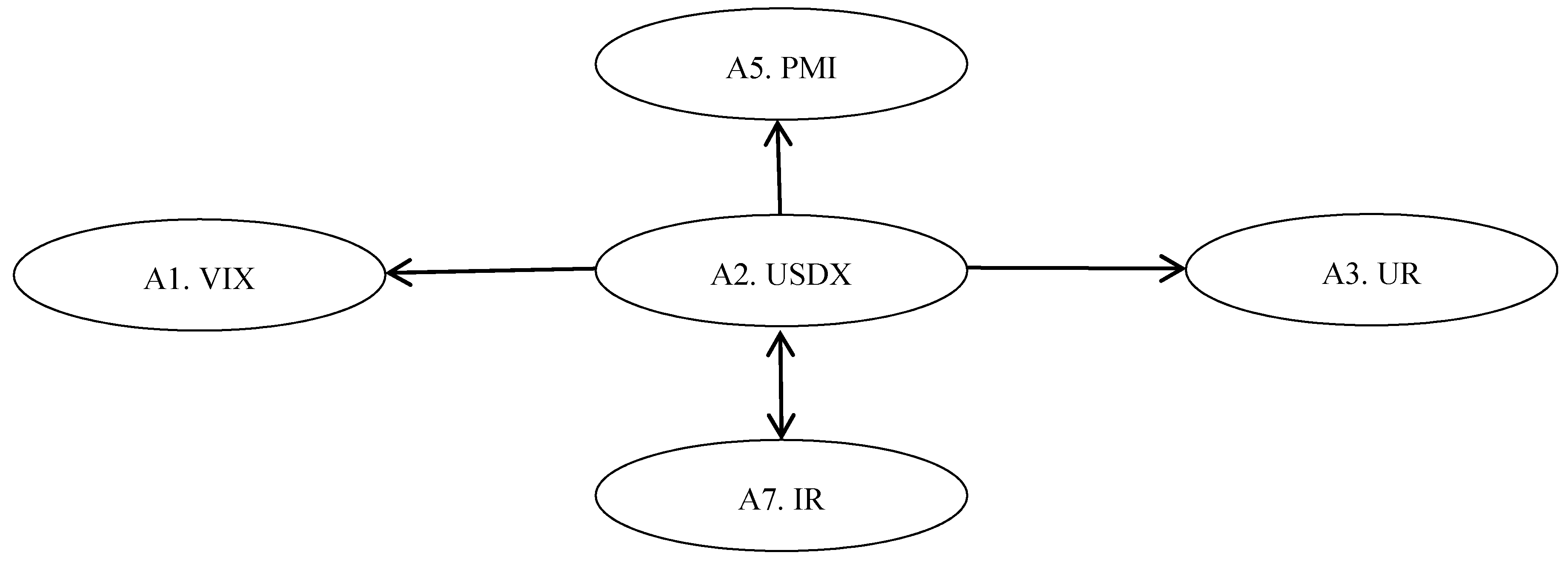
Stage 7. Generating a causal diagram for five core factors

A causal diagram for the five core factors was depicted below:

Figure 5 depicted that (1) the interest rate and US dollar index are mutually affected; and (2) the US dollar index unilaterally affects the ISM manufacturing PMI, unemployment rate, and volatility index.

Our results suggest that investors should pay attention to the change in interest rates when investing in S&P 500 index futures.

4.3. Result Confirmation with Econometric Model

4.3.1. Data Type and Illustration

Table 14. Definition of variables.

Type Variables	Original Data	Natural Log	n-th Differentiation
S&P 500 Stock Index	SNP	LSNP	DLSNP
US Dollar Index	USDX	LUSDX	DLUSDX
Interest Rate	IR	LIR	DLIR
Manufacturing PMI	PMI	LPMI	DLPMI
Volatility	VIX	LVIX	DLVIX
Unemployment Rate	UR	LUR	DLUR

summarized the definition of six variable.

4.3.2. Descriptive Statistics and Sample Period

Table 15. Summary of descriptive statistics.

Statistic	SNP	USDX	IR	PMI	VIX	UR
Mean	1453.337	104.3818	1.259187	52.06504	20.40984	6.925203
Median	1388.200	102.3880	0.16	52.60000	17.43000	6.700000
Maximum	2121.600	125.1504	5.26	59.90000	62.64000	10.00000
Minimum	752.1000	94.59510	0.07	33.10000	10.82000	4.400000
Std. Dev.	352.0651	6.787668	1.950997	5.047755	9.421310	1.881602
Skewness	0.362936	1.104612	1.309019	−1.664707	2.226969	0.153495
Kurtosis	2.295392	3.806274	2.896916	6.601291	8.966264	1.531276
J-B Value	5.244736	28.34508	35.18186	123.2782	284.0985	11.53839
p-Value	0.0726	0.0000 ***	0.0000 ***	0.0000 ***	0.0000 ***	0.0031 ***
No. of Obs	123	123	123	123	123	123

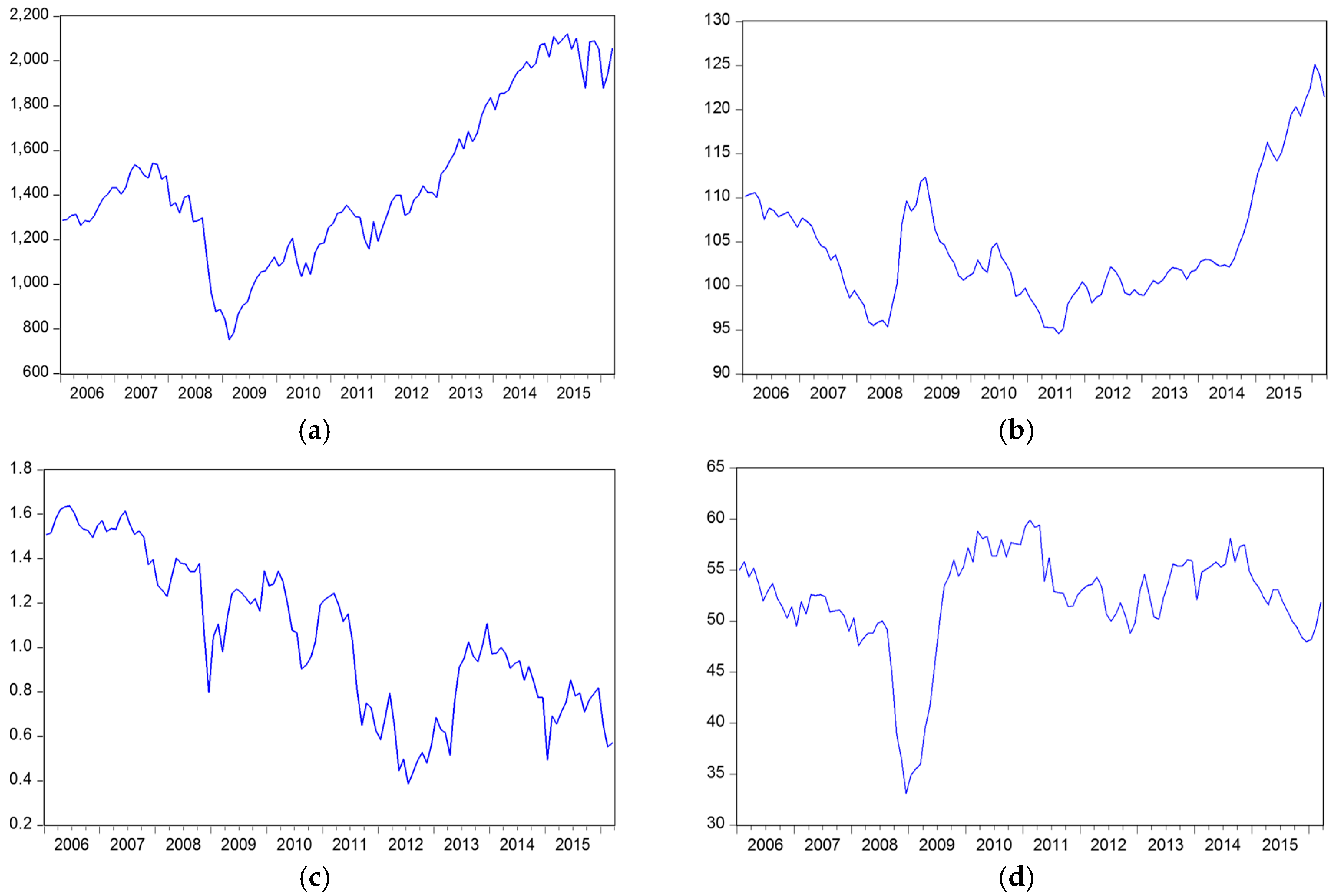
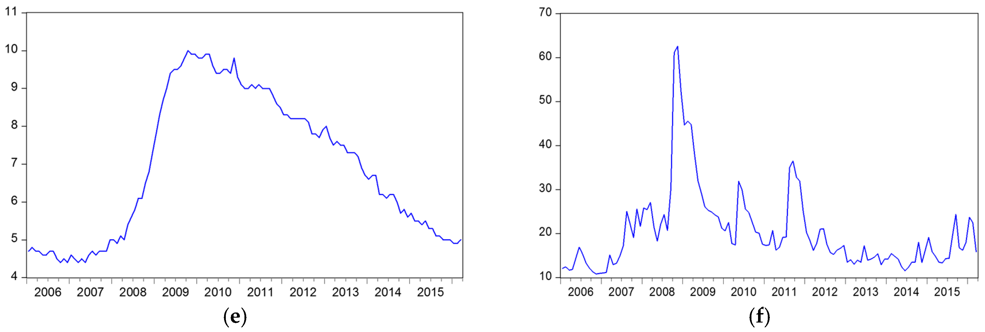
*** demonstrates 1% significance level.

denotes that the skewness of all factors except PMI are positive, suggesting that PMI is skewed left; that means the left tail of PMI is longer than the right side, and the other five factors are skewed to the right. Regarding the kurtosis, we found that S&P 500, interest rate, and unemployment rate are platykurtic distributious (i.e., data distribution with a kurtosis is less than three), and the other three factors are leptokurtic distributions (i.e., data distributions with a kurtosis higher than three). Figure 6. depicts original time series charts for each parameter.

4.3.3. ADF Test

Table 16. Results for the augmented Dicky-Fuller (ADF) test.

Variables	Original (p-Value)	Stationary or Not	1st-order Difference	Stationary or Not	2nd-Order Difference	Stationary or Not
LSNP	0.8873	No	0.0000 ***	Yes	-	-
LUSDX	0.5582	No	0.0000 ***	Yes	-	-
LIR	0.3451	No	0.0000 ***	Yes	-	-
LPMI	0.0198	No	0.0000 ***	Yes	-	-
LVIX	0.0604	No	0.0000 ***	Yes	-	-
LUR	0.0273	No	0.0733	No	0.0000 ***	Yes

Note: *** represents 1% significance level.

denotes that all original data are non-stationary, capable of influencing the behavior of this time series. This first-order difference is taken and all data except unemployment rate under the 1st-order difference column become stationary-order difference for unemployment rate is than taken and unemployment rate under “second-order difference” column of Table 16 become stationary. This result suggests the feasibity of investigating the long-run equilibrium relationship by using the co-integration test [40].

4.3.4. Co-Integration Test Result

Table 17. Result for the co-integration test.

Null Hypothesis	Eigen-Value	Trace Test
		${\mathit{\lambda }}_{\mathit{t}\mathit{r}\mathit{a}\mathit{c}\mathit{e}}$	5% Critical Value
None	0.414595	184.0040 **	134.6780
At most 1	0.331531	119.2144 **	103.8473
At most 2	0.186712	70.4798	76.9728
At most 3	0.139662	45.4727	54.0790
At most 4	0.108124	27.2707	35.1928
At most 5	0.067203	13.4250	20.2618
At most 6	0.040537	5.0072	9.1645

Notes: ** denotes 5% significance level.

denotes that at least two co-integration relationships exist among the six factors.

4.3.5. The Lagged Period for Unemployment Rate and VECM Result

Table 18. The result for the lagged period for unemployment rate.

Lagged Period	0	1	2	3	4	5
SIC	−6.74764	−19.48315 *	−18.68359	−17.99020	−16.52631	−15.48458

Note: * indicates the optimum lagged period based on Schwartz Information Criteria (SIC) rule.

demonstrates that the correction error term to unemployment rate has a significantly negative effect at 1-lag period, where Schwartz Information Criteria (SIC) deals with the optimum lag length..

Table 19. The adjustment speed.

Lagged Period	SNP	USDX	IR	PMI	UR	VIX
Adj. Speed	−0.0612	−0.0097	−0.0587	−0.0967	−0.6488 ***	0.6735
t-Value	−0.7166	−0.3948	−0.3196	−1.4733	−6.1779	1.9556

Note: *** represents 1% significance level.

denotes that unemployment rate was easily modified to the long-run equilibrium with S&P 500 index futures, while the other four parameters was not easily modified to the long-run equilibrium with S&P 500 index futures.

4.3.6. Granger Causality Test results

Table 20. Granger causality test results.

	Dependent Variables	SNP	USDX	IR	PMI	VIX	UR
Independent Variables
SNP		-	0.4291	0.0845	0.1536	0.2931	0.7442
USDX		0.0136 **	-	0.9094	0.4289	0.0039 **	0.2321
IR		0.0086 **	0.0039 **	-	0.7858	0.0033 **	0.6724
PMI		0.0143 **	0.6203	0.0054 **	-	0.1571	0.1195
VIX		0.8223	0.0844	0.8577	0.5590	-	0.4642
UR		0.9998	0.1163	0.8669	0.4011	0.4035	-

Note: ** denotes 5% significance level.

shows that the US dollar index unilaterally affects S&P 500 and VIX index; the interest rate unilaterally affects S&P 500, US dollar index, and VIX index; and the PMI unilaterally affects S&P 500 and interest rate.

4.3.7. Regression Model Confirmation

This study then chooses the top five factors selected by the D-ANP (i.e., US dollar index, interest rate, ISM manufacturing PMI, VIX, and unemployment rate) to be the independent variables, and the rate of return on S&P 500 index futures to be the dependent variable to establish a regression model. The sample period starts from 1 January 2006 to December 2014. The estimated results are summarized below:

$${\widehat{R}}_{1t}=0.005-0.813USD{X}_{1t}+0.068I{R}_{1t}+0.012PM{I}_{1t}-0.14VI{X}_{1t}-0.07U{R}_{1t}$$

(0.067 *) (0.002 ***) (0.035 **) (0.891) (0.000 ***) (0.056 *)

Empirical findings indicate that the volatility index, US dollar index, and unemployment rate have significantly negative relationships with S&P 500 index. This result suggests that the investors expect a decrease in S&P 500 index when VIX, US dollar index, and unemployment rate increase. However, the interest rate has a significant positive relationship with S&P 500 index, suggesting that S&P 500 index rises when the the interest rate increases, suggesting that there is an optimism about a future business boom, so that the S&P 500 index rises as a result.

Empirical results also prove that the factors chosen via the D-ANP are not significantly different from those obtained using the regression model, implying that S&P 500 investment decisions based on the D-ANP have similarly explanatory power to those obtained from the regression model.

4.3.8. GRA

For GRA, the GRC is computed to demonstrate the relationship between the ideal and the actual empirical findings. A multi-criteria problem is defined using a set of choices (x₁, x₂, …, x_m) with n criteria. The GRC, ${\mathsf{\xi }}_k$(x_i, x_j), is expressed as

$${\xi }_k\left(x_i,x_j\right)=\frac{{\Delta }_{min}+\rho {\Delta }_{max}}{{\Delta }_{jik}+\rho {\Delta }_{max}}$$

(9)

where x_i denotes a reference sequence, and x_j represents a comparative sequence; ${\Delta }_{jik}$ is defined as the grey relational space, and ξ_k(x_i, x_j) is between 0 and 1.

$$\Delta \min =\begin{array}{c}\min \\ s\end{array}\begin{array}{c}\min \\ l\end{array}\left|xil-xsl\right|,1\le s\le m,1\le l\le n,$$

(10)

$$\Delta \max =\begin{array}{c}\max \\ s\end{array}\begin{array}{c}\max \\ l\end{array}\left|xil-xsl\right|,1\le s\le m,1\le l\le n,$$

(11)

$$\Delta jik=\left|xik-xjk\right|,$$

(12)

where | . | denotes the absolute value and ρ is the distinguishing coefficient (0 ≤ ρ ≤ 1). Liu and Lin [2] reported that ρ = 0.5 is normally applied.

After obtaining the GRC, its mean value is often used as the GRG, γ(x_i, x_j):

$$\mathsf{\gamma }\left(x_i,x_j\right)={\displaystyle \sum }_{k=1}^n{w}_k{\xi }_k\left(x_i,x_j\right),$$

(13)

where γ(x_i, x_j) represents GRG for the i^th experiment, and j shows the number of performance characteristics (taking value between 0 and 1), w_k denotes the relative weight of performance characteristic k; and w₁, w₂, …, w_n are usually satisfied as:

$${\displaystyle \sum }_{j=1}^n{w}_j=1$$

(14)

5. Result Confirmation Using GRA

We invited 13 experts to choose 12 factors affecting S&P 500 index futures using the Delphi method and then calculated the weight for each factor via the D-ANP. However, the empirical results show that incomplete information and uncertain relations may exist among the chosen factors. Therefore, we applied GRA to examine four major S&P 500 sectors and to investigate three major US stock indexes to confirm that the 12 factors chosen via the D-ANP are appropriate.

5.1. Using GRA to Measure the Explanatory Power for Four Major S&P 500 Sectors

(1) Determine the reference series and comparative series

We asked 13 experts to rank the scores for four major S&P 500 sectors. The ranking score is ranged from 0 to 100, where 0 denotes no forecasting power, 50 indicates fair forecasting power, and 100 represents extremely strong forecasting power.

Table 21. Original data for 12 factors for four S&P 500 sectors.

Factors	VIX	USDX	UR	IPI	PMI	CPI	IR	KD	DMI	TV	MA	OI
Symbol	(A1)	(A2)	(A3)	(A4)	(A5)	(A6)	(A7)	(B1)	(B2)	(B3)	(B4)	(B5)
E	75.455	82.727	76.818	80.909	76.364	69.091	77.273	61.818	64.091	73.182	68.636	63.182
F	70.455	77.273	67.273	75.000	75.000	65.455	78.182	55.909	61.818	66.818	60.455	60.000
G	67.273	74.545	70.909	64.545	65.455	63.636	71.364	53.182	57.273	65.000	61.364	58.182
H	75.455	84.091	75.909	68.545	76.364	77.727	85.909	58.182	64.091	70.909	65.000	62.727

summarizes the scores for the 12 factors given by the 13 experts. E denotes the Industrials, F the Transportation, G the Utility, and H the financial sector of the S&P 500 index.

Table 22. The reference and comparative series for 12 factors for four S&P 500 sectors.

Factors	VIX	USDX	UR	IPI	PMI	CPI	IR	KD	DMI	TV	MA	OI
Symbol	(A1)	(A2)	(A3)	(A4)	(A5)	(A6)	(A7)	(B1)	(B2)	(B3)	(B4)	(B5)
X0	75.455	84.091	76.818	80.909	76.364	77.727	85.909	61.818	64.091	73.182	68.636	63.182
E	75.455	82.727	76.818	80.909	76.364	69.091	77.273	61.818	64.091	73.182	68.636	63.182
F	70.455	77.273	67.273	75.000	75.000	65.455	78.182	55.909	61.818	66.818	60.455	60.000
G	67.273	74.545	70.909	64.545	65.455	63.636	71.364	53.182	57.273	65.000	61.364	58.182
H	75.455	84.091	75.909	68.545	76.364	77.727	85.909	58.182	64.091	70.909	65.000	62.727

summarizes the reference and comparative series. The reference series (X₀) is the maximum value for the four sectors of each factor, and the original data for each sector serves as the comparative series.

(2) Calculate the GRC values for four S&P 500 sectors

Table 23. The GRC values for 12 factors for four S&P 500 sectors.

Factors	VIX	USDX	UR	IPI	PMI	CPI	IR	KD	DMI	TV	MA	OI
Symbol	(A1)	(A2)	(A3)	(A4)	(A5)	(A6)	(A7)	(B1)	(B2)	(B3)	(B4)	(B5)
E	1.000	0.605	0.891	0.671	0.925	0.636	0.860	0.450	0.495	0.831	0.620	0.476
F	0.690	0.860	0.576	0.961	0.961	0.527	0.803	0.363	0.450	0.563	0.426	0.419
G	0.576	0.925	0.710	0.505	0.527	0.485	0.731	0.333	0.380	0.516	0.441	0.392
H	1.000	0.563	0.961	0.617	0.925	0.831	0.516	0.392	0.495	0.710	0.516	0.467

lists the GRC values for 12 factors for four S&P 500 sectors according to Equation (1).

(3) Calculate the GRG values and ranking for four S&P 500 sectors

We then calculated the GRG values for 12 factors for each sector. The weight for each factor ($w_b$) was calculated using Borda’s count [42]. Replacing the weights into Equation (5), we obtain the GRG values listed in

Table 24. The grey relational grade (GRG) values for 12 factors and ranking order for four S&P 500 sectors.

Factors	VIX	USDX	UR	IPI	PMI	CPI	IR	KD	DMI	TV	MA	OI	GRG	Ranking
Symbol	(A1)	(A2)	(A3)	(A4)	(A5)	(A6)	(A7)	(B1)	(B2)	(B3)	(B4)	(B5)
Wb	0.065	0.016	0.065	0.081	0.048	0.113	0.032	0.145	0.129	0.097	0.129	0.081
E	0.065	0.039	0.057	0.043	0.060	0.041	0.055	0.029	0.032	0.054	0.040	0.031	0.546	1
F	0.045	0.055	0.037	0.062	0.062	0.034	0.052	0.023	0.029	0.036	0.027	0.027	0.490	3
G	0.037	0.060	0.046	0.033	0.034	0.031	0.047	0.022	0.025	0.033	0.028	0.025	0.421	4
H	0.065	0.036	0.062	0.040	0.060	0.054	0.033	0.025	0.032	0.046	0.033	0.030	0.516	2

. Table 24 summarizes the GRG rankings for four S&P 500 sectors: E > H > F > G. This suggests that the 13 experts deemed that the explanatory power of 12 factors is strongest for the S&P 500 industrial sector, followed by the financial, transportation, and utility sectors.

5.2. Using GRA to Measure the Explantory Power for Three Major US Stock Indexs

(1) Determine the reference and comparative series

We asked 13 experts to measure the explanatory power for three major US stock indexes: Dow Jones, NASDAQ 100, and S&P 500. The possible score ranges from 0 to 100, where 0 denotes no forecasting power, 50 indicates fair forecasting power, and 100 represents extremely strong forecasting power.

Table 25. Original data for the 12 factors for three major US stock indexes.

Factors	VIX	USDX	UR	IPI	PMI	CPI	IR	KD	DMI	TV	MA	OI
Symbol	(A1)	(A2)	(A3)	(A4)	(A5)	(A6)	(A7)	(B1)	(B2)	(B3)	(B4)	(B5)
J	81.818	85.000	80.455	80.455	82.273	78.182	85.455	69.091	75.000	76.364	71.364	72.273
K	82.727	85.455	81.364	80.000	82.727	78.636	85.909	59.091	62.273	66.818	60.909	63.182
L	82.273	82.273	81.818	80.000	81.364	77.727	84.091	58.182	61.364	65.455	62.273	65.909

lists the original data series formed by the average score for each factor given by 13 experts for the stock indexes: J denotes S&P 500, K denotes NASDAQ 100, and L denotes Dow Jones Industrial index futures.

Table 26. Reference and comparative series for the 12 factors for three major US stock indexes.

Factors	VIX	USDX	UR	IPI	PMI	CPI	IR	KD	DMI	TV	MA	OI
Symbol	(A1)	(A2)	(A3)	(A4)	(A5)	(A6)	(A7)	(B1)	(B2)	(B3)	(B4)	(B5)
X0	82.727	85.455	81.818	80.455	82.727	78.636	85.909	69.091	75.000	76.364	71.364	72.273
J	81.818	85.000	80.455	80.455	82.273	78.182	85.455	69.091	75.000	76.364	71.364	72.273
K	82.727	85.455	81.364	80.000	82.727	78.636	85.909	59.091	62.273	66.818	60.909	63.182
L	82.273	82.273	81.818	80.000	81.364	77.727	84.091	58.182	61.364	65.455	62.273	65.909

shows that the comparative series are the original data for three US stock index futures, and the reference series ($X_0$) is the maximum value of these three stock indexes for each factor.

(2) Calculate the GRC values for three major US stock indexes: We used Equation (1) to calculate the GRC values as shown in

Table 27. Grey relational coefficient (GRC) values for the 12 factors for three major US stock indexes.

Factors	VIX	USDX	UR	IPI	PMI	CPI	IR	KD	DMI	TV	MA	OI
Symbol	(A1)	(A2)	(A3)	(A4)	(A5)	(A6)	(A7)	(B1)	(B2)	(B3)	(B4)	(B5)
J	2.793	2.531	2.531	2.531	2.893	2.189	2.455	1.421	1.841	1.976	1.558	1.620
K	3.000	2.455	2.700	2.455	3.000	2.250	2.382	1.025	1.125	1.306	1.080	1.157
L	2.893	2.893	2.793	2.455	2.700	2.132	2.700	1.000	1.095	1.246	1.125	1.266

.

(3) Calculate the GRG values for three US major stock indexes: We then calculated the GRG values for the 12 factors for three major US stock indexes using Equation (5), as shown in

Table 28. The GRG values for the 12 factors and ranking order for three major US stock indexes.

Rules	VIX	USDX	UR	IPI	PMI	CPI	IR	KD	DMI	TV	MA	OI	GRG	Ranking
Symbol	(A1)	(A2)	(A3)	(A4)	(A5)	(A6)	(A7)	(B1)	(B2)	(B3)	(B4)	(B5)
Wb	0.065	0.016	0.065	0.081	0.048	0.113	0.032	0.145	0.129	0.097	0.129	0.081
J	0.180	0.163	0.163	0.163	0.187	0.141	0.158	0.092	0.119	0.127	0.100	0.105	1.699	1
K	0.194	0.158	0.174	0.158	0.194	0.145	0.154	0.066	0.073	0.084	0.070	0.075	1.544	3
L	0.187	0.187	0.180	0.158	0.174	0.138	0.174	0.065	0.071	0.080	0.073	0.082	1.568	2

.

The GRG ranking order for the three major US stock indexes futures indicate that 13 experts deemed that the 12 factors have the strongest explanatory power in forecasting S&P 500 index futures, followed by the Dow Jones Industrial index futures, with the lowest explanatory power for NASDAQ 100 index futures.

6. Conclusions

We combined the D-ANP with GRA to examine the key factors for investor trading in S&P 500 index futures and mutual relationships among key factors. We can draw the following conclusions.

• Thirteen experts picked five key factors out of 19 factors affecting investor trading in S&P 500 index futures. These key factors were the US dollar index, interest rate, ISM manufacturing PMI, volatility index, and unemployment rate. We found that the US dollar index is the most important among these five key factors.
• Previous studies concentrated on the explanatory power of technical indicators for S&P 500 index futures. Here, we found a weight for each key factor using the D-ANP, and we also considered various macroeconomic factors, which were found to have more explanatory power than those of technical factors found in previous research papers.
• The D-ANP results revealed that the interest rate and US dollar index have mutually causal relationships, while the US dollar index unilaterally affects ISM manufacturing PMI, volatility index, and unemployment rates.
• The co-integration results showed that there were at least two co-integration relationships that existed among the six factors. We also found that the correction term to unemployment rate has a significantly negative effect at 1-lag period, and we found that the unemployment rate was easily modified to the long-run equilibrium.
• Granger causality test results confirmed some similar results obtained via the D-ANPs that the US dollar index, interest rate, and the ISM manufacturing PMI have major impacts on the S&P 500 index futures.
• The general regression results also confirmed that four out of the five factors selected via the D-ANP (volatility index, US dollar index, interest rate, and unemployment rate) have strong explanatory power in forecasting S&P 500 index futures.
• We used the GRA to examine the explanatory power of the 12 factors selected by the D-ANP for different S&P 500 sectors. Empirical results indicated that the 12 factors had the strongest explanatory power for S&P 500 Industrial sector and the least explanatory power for S&P 500 Utility sector.
• We applied the GRA to measure the explanatory power of the 12 factors selected via the D-ANP for three major US stock indexes futures. Empirical findings showed that the 12 factors had the strongest explanatory power in forecasting S&P 500 index futures, while the least explanatory power in forecasting NASDAQ 100 index futures.

References

- Tzeng, G.H.; Huang, J.J. Multiple Attribute Decision Making: Methods and Applications; CRC Press: Boca Raton, FL, USA, 2011. [Google Scholar]
- Liu, S.; Lin, Y. Grey Information: Theory and Practical Applications; Springer: London, UK, 2010. [Google Scholar]
- Saaty, T.L. The Analytic Network Process—Decision Making with Dependence and Feedback; RWS Publications: Pittsburgh, PA, USA, 1996. [Google Scholar]
- Coulter, K.; Sarkis, J. Development of a media selection model using the analytic network process. Int. J. Advert. 2005, 24, 193–216. [Google Scholar] [CrossRef]
- Kahraman, C.; Ertay, T.; Buyukozkan, G. A fuzzy optimization model for QFD planning process using Analytical Network Approach. Eur. J. Oper. Res. 2006, 171, 390–411. [Google Scholar] [CrossRef]
- Kou, G.; Ergu, D. AHP/ANP theory and its application in technology and economic development: The 90th anniversary of Thomas L. Saaty. Technol. Econ. Dev. Econ. 2016, 22, 649–650. [Google Scholar] [CrossRef]
- Kou, G.; Ergu, D.; Lin, C.; Chen, Y. Pairwise comparison matrix in multiple criteria decision making. Technol. Econ. Dev. Econ. 2016, 22, 738–765. [Google Scholar] [CrossRef]
- Liao, C.N.; Fu, Y.K.; Wu, L.C. Integrated FAHP, ARAS-F and MSGP Methods for green supplier evaluation and selection. Technol. Econ. Dev. Econ. 2016, 22, 670–684. [Google Scholar] [CrossRef]
- Sekitani, K.; Takahashi, I. A unified model and analysis for AHP and ANP. J. Oper. Res. Soc. Jpn. 2001, 44, 67–89. [Google Scholar] [CrossRef]
- Shee, D.Y.; Tzeng, G.H.; Tang, T.I. AHP, fuzzy measure and Fuzzy integral approaches for the appraisal of information service providers in Taiwan. J. Glob. Inf. Technol. Manag. 2003, 6, 8–30. [Google Scholar] [CrossRef]
- Shieh, L.F.; Yeh, C.C.; Lai, M.C. Critcal success factors in digital publishing technology using an ANP approach. Technol. Econ. Dev. Econ. 2016, 22, 670–684. [Google Scholar] [CrossRef]
- Hu, Y.C. Analytic network process for patten classification problems using genetic algorithms. Inf. Sci. 2010, 180, 2528–2539. [Google Scholar] [CrossRef]
- Moghaddam, N.B.; Sahafzadeh, M.; Alavijeh, A.S.; Yousefdehi, H.; Hosseini, S.H. Strategic environment analysis using DEMATEL method through systematic approach: Case study of an energy research institute in Iran. Manag. Sci. Eng. 2010, 4, 95–105. [Google Scholar]
- Herat, A.T.; Noorossana, R.; Parsa, S.; Serkani, E.S. Using DEMATEL-Analytic Network Process (ANP) hybrid algorithm approach for selecting improvement projects of Iranian excellence model in healthcare. Afr. J. Bus. Manag. 2012, 6, 627–645. [Google Scholar]
- Hu, J.W.S.; Hu, Y.C.; Yang, T.P. Evaluating the optimum strategy developed by combining Jesse L. Livermore’s key price logic and the D-ANPs. Univeral J. Account. Financ. 2017, 5, 18–35. [Google Scholar]
- Hu, K.H.; Wei, J.G.; Tzeng, G.H. Risk factor assessment improvement for China’s cloud computing auditing using a new hybrid MADM model. Int. J. Inf. Technol. Decis. Mak. 2017, 16, 737–777. [Google Scholar] [CrossRef]
- Hu, Y.C.; Chiu, Y.J.; Hsu, C.S.; Chang, Y.Y. Identifying key factors of introducing GPS-based fleet management systems to the logistics industry. Math. Probl. Eng. 2015, 2015. [Google Scholar] [CrossRef]
- Liou, J.J.H.; Tamošaitiené, J.; Zavadskas, E.K.; Tzeng, G.H. New hybrid COPRAS-G-MADM Model for improving and selecting suppliers in green supply chain management. Int. J. Prod. Res. 2016, 51, 114–134. [Google Scholar] [CrossRef]
- Ou Yang, Y.P.; Shieh, H.M.; Leu, J.D.; Tzeng, G.H. A novel hybrid MCDM model combined with DEMATEL and ANP with applications. Int. J. Oper. Res. 2008, 5, 160–168. [Google Scholar]
- Shen, K.Y.; Tzeng, G.H. Combining DRSA decision-rules with FCA-based DANP evaluation for financial performance improvements. Technol. Econ. Dev. Econ. 2016, 22, 685–714. [Google Scholar] [CrossRef]
- Vujanović, D.; Momčilović, V.; Bojović, N.; Papić, V. Evaluation of vehicle fleet maintenance management indicators by application of DEMATEL and ANP. Expert Syst. Appl. 2012, 39, 10552–10563. [Google Scholar] [CrossRef]
- Deng, J. Control problems of Grey System. Syst. Control Lett. 1982, 5, 288–294. [Google Scholar]
- Deng, J. Introduction to Grey System Theory. J. Grey Syst. 1989, 1, 1–24. [Google Scholar]
- Chan, T.W.K.; Tong, T.K.L. Multi-criteria material selections and end-of-life product strategy: Grey relational analysis approach. Mater. Des. 2007, 28, 1539–1546. [Google Scholar] [CrossRef]
- Chen, H.C.; Hu, Y.C.; Shyu, J.Z.; Tzeng, G.H. Comparing possibility grey forcecasting with neural network-based fuzzy regression by an empirical study. J. Grey Syst. 2005, 8, 93–106. [Google Scholar]
- Guo, Y.; Yang, T.; Huang, G.W. The use of grey relational analysis in solving multiple attribute decision-making problems. Comput. Ind. Eng. 2008, 55, 80–93. [Google Scholar]
- Hasani, H.; Tabatabaei, S.A.; Amiri, G. Grey relational analysis to determine the optimum process parameters for open-end spinning yarns. J. Eng. Fibers Fabr. 2012, 7, 81–86. [Google Scholar]
- Hu, Y.C.; Jiang, P. Forecasting energy demand using neural-network-based grey residual modification models. J. Oper. Res. Soc. 2017, 68, 556–565. [Google Scholar] [CrossRef]
- Hu, Y.C. Pattern classification using grey tolerance rough sets. Kybernetes 2016, 45, 266–281. [Google Scholar] [CrossRef]
- Hu, Y.C.; Chen, R.S.; Hsu, Y.T.; Tzeng, G.H. Grey self-organizing feature maps. Neurocomputing 2002, 48, 863–877. [Google Scholar] [CrossRef]
- Huang, J.T.; Liao, Y.S. Application of grey relationship analysis to machining parameter determination of wire electrical discharge machining. Int. J. Prod. Res. 2003, 41, 90–102. [Google Scholar]
- Huang, S.J.; Chiu, N.H.; Chen, L.W. Integration of the grey relational analysis with genetic algorithm for software effort estimation. Eur. J. Oper. Res. 2008, 188, 898–909. [Google Scholar] [CrossRef]
- Kung, C.Y.; Wen, K.L. Applying grey relational analysis and grey decision-making to evaluate the relationship between company attributes and its financial performance-A case study of venture capital enterprises in Taiwan. Decis. Support Syst. 2007, 43, 842–852. [Google Scholar] [CrossRef]
- Lin, C.L. Use of the Taguchi method and grey relational analysis to optimize turning operations with multiple performance characteristics. J. Mater. Manuf. Process. 2004, 19, 209–220. [Google Scholar] [CrossRef]
- Pakkar, M.S. An integrated approach to grey relational analysis, analytic hierarchy process and data envelopment analysis. J. Cent. Cathera 2016, 9, 71–86. [Google Scholar] [CrossRef]
- Tan, X.; Li, Y. Using grey relational analysis to analyze the medical data. Kybernetes 2004, 33, 355–362. [Google Scholar]
- Yamaguchi, D.; Li, G.D.; Nagai, M. New grey relational analysis for finding the invariable structure and its application. J. Grey Syst. 2005, 8, 167–178. [Google Scholar]
- Gordon, T.J.; Helmer, O. Report on a Long-Range Forecasting Study; The RAND Corporation: Santa Monica, CA, USA, 1964. [Google Scholar]
- Görener, A. Comparing AHP and ANP: An application of strategic decisions making in a manufacturing company. Int. J. Bus. Soc. Sci. 2012, 3, 194–208. [Google Scholar]
- Johansen, S.; Juselius, K. Maximum likelihood estimation and inference of economics and statistics. Oxf. Bull. Econ. Stat. 1990, 52, 169–210. [Google Scholar] [CrossRef]
- Saari, D.G. Mathematic structure of voting paradoxes. Econ. Theory 2000, 15, 1–53. [Google Scholar] [CrossRef]
- Borda, J.C. A paper on elections by ballot. In Condorcet: Foundations of Social Choice and Political Theory; Hewitt, F., Mclean, I., Eds.; Edward Elgar: Brookfield, WI, USA, 2004; pp. 114–119. [Google Scholar]
Figure 1.
The prototypical structure. (MSCI: Morgan Stanley Capital International; GNP: Gross National Product; K.D.: Stochastic Oscillator).