Semi–Automatic Corpus Callosum Segmentation and 3D Visualization Using Active Contour Methods

Abstract

Accurate 3D computer models of the brain, and also of parts of its structure such as the corpus callosum (CC) are increasingly used in routine clinical diagnostics. This study presents comparative research to assess the utility and performance of three active contour methods (ACMs) for segmenting the CC from magnetic resonance (MR) images of the brain, namely: an edge-based active contour model using an inflation/deflation force with a damping coefficient (EM), the Selective Binary and Gaussian Filtering Regularized Level Set (SBGFRLS) method and the Distance Regularized Level Set Evolution (DRLSE) method. The pre-processing methods applied during research work were to improve the contrast, reduce noise and thus help segment the CC better. In this project, 3D CC models reconstructed based on the segmentations of cross-sections of MR images were also visualised. The results, as measured by quantitative tests of the similarity indice (SI) and overlap value (OV) are the best for the EM model (SI = 92%, OV = 82%) and are comparable to or better than those for other methods taken from a literature review. Furthermore, the properties of the EM model consisting in its ability to both expand and shrink at the same time allow segmentations to be better fitted in subsequent CC slices then in state-of-the art ACMs such as DRLSE or SBGFRLS. The CC contours from previous and subsequent iterations produced by the EM model can be used for initiation in subsequent or previous frames of MR images, which makes the segmentation process easier, particularly as the CC area can increase or decrease in subsequent MR image frames.

1. Introduction

The human brain is composed of anatomical regions with various, complex and interrelated functions. The appropriate volumetric measurements and high quality brain tissue visualisation allow an assessment of the pathologies that occur. This is why brain image segmentation and also the computer-aided classification of lesions play a very important role [1,2,3,4,5,6,7].

The corpus callosum (CC) is the largest structure of white matter in the human brain, made of axon fibres intersecting the left and right hemispheres [8]. Neuropathological examinations have shown that various neurological disorders frequently cause changes to the structure and size of the corpus callosum. In particular, it applies to diseases such Alzheimer’s [9] or multiple sclerosis [10]. Consequently, an accurate segmentation of the CC and then its 3D reconstruction and visualisation is of great significance in diagnosing and then treating the patient. For this purpose, it is important to create new computer methods and also to develop existing approaches allowing better and more accurate results to be obtained.

Magnetic Resonance Imaging (MRI) ensures high contrast between various soft tissues, so it is the preferred method of examining the brain, including the CC. In T1-weighted MR images of the brain, acquired in the sagittal plane, the CC has a curved, elongated shape of the inverted letter C, with a high intensity of pixels. An example CC image in the sagittal plane is shown in Figure 1.

Manually tracing the CC in MR images is time-consuming, difficult and requires specialized training. This is why computer segmentation methods are of great practical significance, as they support the work of physicians and may help them make the right diagnosis.

The active contour method (ACM) is a valuable tool for segmenting regions of interest (ROIs) in medical images. In this study, three ACMs were used in this study to segment the CC in magnetic resonance images of the brain, namely:

(1)

An edge-based active contour model using an inflation/deflation force with a damping coefficient (EM) [12].

(2)

Two state-of-the-art level-set ACMs [13,14]; distance regularized level set evolution (DRLSE) method [13]; selective Binary and Gaussian Filtering Regularized Level Set (SBGFRLS) method [14]. Authors of publications [13,14] presented high results of CC segmentation in single slices from brain MRIs.

The CC segmentation with the use of models [12,13,14] was carried out in subsequent cross-sections in the midsagittal plane of MRIs. This made it possible to assess the utility of these models for a segmentation followed by the 3D reconstruction and visualisation of the CC. The ACM models used allow a semi-automatic segmentation because the seed contour must be identified in each test set and this contour is then to fit the CC edge being detected. A method which segments automatically requires no initial parameters and/or contours/points in the test set.

The original contribution of this paper consists in: (1) presenting an algorithm of the EM model in which an iteration equation for the movement of active contour points and a method of determining new points have been proposed. These solutions, plus the pre-processing method employed, have decreased the number of operations and parameters used, shortened the evolution time of the active contour, and allowed a smoother and more accurately approximated CC edge to be produced than by the approach from previous research [12,15]. (2) Developing a tool for segmenting and 3D-visualising the CC using the following open-source software systems: Insight Segmentation and Registration Toolkit (ITK) [16], the Visualization Toolkit (VTK) [17] and ITK-SNAP [18]; (3) Evaluating the segmentation results produced by the EM model compared to two other ACMs implemented, namely: DRLSE, SBGFRLS; (4) Using the knowledge of a physician, a specialist in human anatomy, at the final step of the segmentations carried out; (5) Proposing a method that makes use of the EM model which produced results of the CC segmentation and then 3D visualisation that are better than from DRLSE and SBGFRLS as well as segmentation results similar to or better than those of other methods taken from the literature review.

This article is structured as follows. In Section 2, we introduce the related studies about CC segmentation. Section 3 contains the Materials and Methods. Section 4 presents the Experimental Results and Discussion. Section 5 presents the Conclusions.

2. Related Works

A literature review allows several groups of methods for segmenting the CC to be distinguished, namely: Model-based methods [19,20,21], Region-based methods [22], Machine learning methods [23,24] and Hybrid methods [25,26].

2.1. Model-Based Methods

These methods segment the image starting with an initial contour or shape and then update this contour/shape in subsequent iterations to the expected final form of the approximated shape (2D or 3D) or approximated edges. The updates are made based on a priori defined knowledge about how these methods determine probable borders of objects. In Ref. [19], the authors proposed non–rigid registration and atlas-based methods for comparing the volume of the cross-sectional area of the midsagittal CC. Adamson et al. [20], in turn, described the application of a template–guided initialisation, followed by its refinement using mathematical morphology operations. Liu and Ruan [21] presented a CC segmentation based on an approach which regularizes the target shape with a level–set based method.

2.2. Region-Based Methods

A technique which segments the image by assessing the similarity of the value of intensity between the adjacent pixels. The segmentation is usually initiated with seed points.

Bueno et al. [22] applied the watershed by immersion segmentation [27] based on a gradient determined in the source images from a magnetic resonance examination of the brain. In previous work [22], the authors described the application of additional morphological operations, such as the use of markers and image reconstruction using an erosion operator to reduce the oversegmentation after the watershed segmentation.

2.3. Machine Learning Methods

Machine learning uses computer algorithms which can learn complex patterns from image data to recognise and/or distinguish defined features that allow segmentation.

In former work [23], a probabilistic 3D shape model based on a training set composed of manually segmented and coaligned images was used to segment the CC. This is followed by a Bayesian segmentation with the use of an identified joint Markov–Gibbs random field model of the MRI. Xu et al. [24] used a Bayesian model-based approach to segment magnetic resonance images. This was followed by the application of the Gibbs sampler based on the Swendsen–Weng method for posterior sampling. The approach introduced in publication [24] makes it possible to segment multiple MR images at the same time.

2.4. Hybrid Methods

Hybrid methods combine different techniques which can come from various groups and categories of methods used in segmentation.

Karsch et al. [25] proposed a 3D method in which the user first has to specify a voxel inside the CC in the MRI. Method [25] combines both region-based and boundary-based approaches. Gass et al. [26] used an approach based on the Markov random field (MRF) to segment 2D midsagittal slices of a brain MRI. In article [26], a two–layer graph was used, where one layer consists of the segmentation, and the second allows the registration.

A summary of the literature review is presented in

Table 1. Methods allowing the corpus callosum (CC) to be segmented from magnetic resonance (MR) images–based on a literature review. The classification also takes into account whether the method enables an automatic [A] or a semi–automatic [S] segmentation.

Class	Author, Year	Method Type
Model-based	Pfefferbaum et al., [19], 2006	[A]
	Adamson et al., [20], 2014	[A]
	Liu and Ruan [21], 2015	[A]
Region-based	Bueno et al., [22], 2001	[S]
Machine learning methods	El–baz et al., [23], 2011	[A]
	Xu et al., [24], 2009	[A]
Hybrid methods	Karsch et al., [25], 2009	[S]
	Gass et al., [26], 2014	[A]

. A more detailed review of literature and the classification of methods allowing the CC to be segmented is presented in publication [28].

3. Materials and Methods

The magnetic resonance images used in this study are in the NIfTI–1 format and come from a public database, namely Minimal Interval Resonance Imaging in Alzheimer’s Disease (MIRIAD) [11]. All scans were acquired with 1.5T Signa MRI scanner (GE Medical systems, Milwaukee, WI, USA). T1-weighted images were obtained with an IR-FSPGR (inversion recovery prepared fast spoiled gradient recalled) sequence (TR/TE/TI = 15/5.4/650 ms), flip angle = 15${}^{\circ }$, slice thickness = 1.5 mm, matrix size = 512 × 512 and field of view = 24 cm × 24 cm.

In this research, MR images from 30 patients (16 male and 14 female) diagnosed with the Alzheimer’s Disease (AD) were used. The age of patients when undergoing the MRI examination was 69.4 ± 7.1 years [11]. Between 10 and maximum 15 slices from every MR examination of a patient were taken for the 3D reconstruction. MR images from five patients (three male and two female) were used as the training set to define the parameters of the pre-processing and segmentation methods applied. The training set made use of 60 midsaggital slices altogether. The training set was selected very carefully by a physician, a specialist in human anatomy, and included CC slices of various sizes and surface areas for the purpose of selecting the right parameters, including the maximum number of iterations necessary to initiate the ACMs. The remaining set of MRIs from 25 patients (13 male and 12 female) was used to test the segmentation methods employed. The test set made use of 325 midsaggital slices altogether.

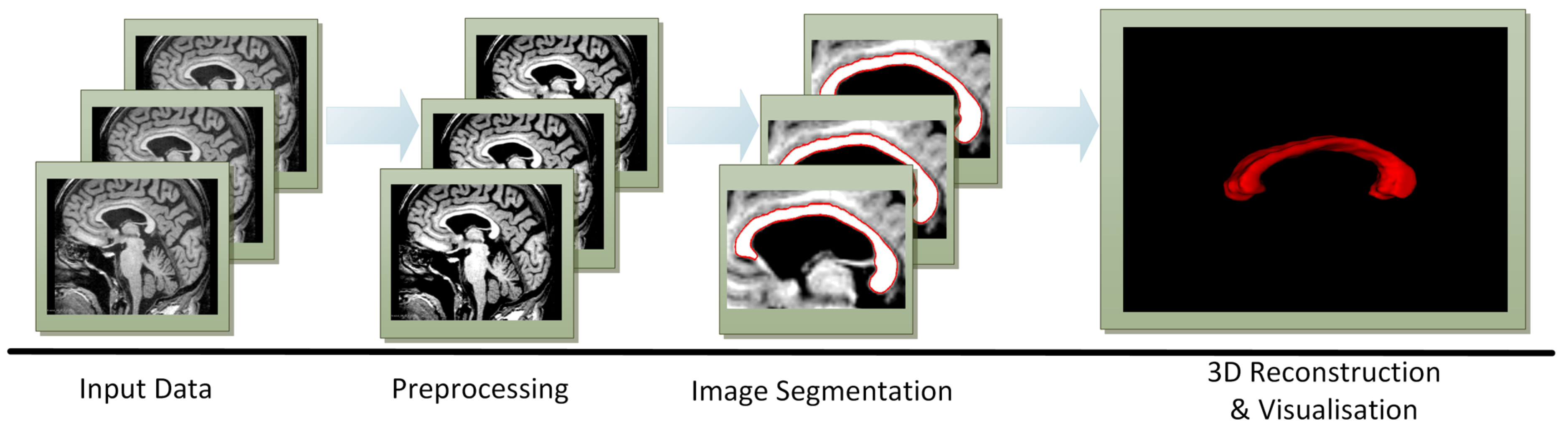
The approach of this research project is illustrated in Figure 2. The pre-processing is to strengthen the contrast of input images and eliminate noise. Then, ACMs are used to segment the CC, which is followed by its reconstruction and visualisation. The 3D reconstruction is made by the marching cubes [29,30] method based on the CC segmentations produced for a defined number of cross-sections from every patient examination. The CC was visualised in 3D using the following environments: Insight Segmentation and Registration Toolkit (ITK) [16], the Visualization Toolkit (VTK) [17] and ITK–SNAP [18].

As a result, the research produced a tool that allows CC slices to be segmented and then 3D visualised, which runs under Windows 10 and Linux (Ubuntu 18.04.1 LTS). Pre-processing methods as well as ACMs, namely—EM, DRLSE, SBGFRLS—have been implemented in C++ (Windows system: Microsoft Visual Studio 2017 environment, under Linux system: GNU Compiler Collection (GCC) gcc-8) and Python (version 3.7.0).

3.1. Pre-Processing

Let I be a grey-level image with intensity values within the interval $(Min,Max)$. Let $I_n$ be a new image with the value interval $(nMin,nMax)$. During pre-processing, the contrast is amplified by rescaling contrast limits of MR images in grey levels to new values using the contrast stretching transformation (normalization) [31], according to the following relationship:

$$I_n=(I-Min)\frac{nMax-nMin}{Max-Min}+nMin.$$

(1)

In the method presented in [31], the $Min$ and $Max$ values are read from the image if image I does not contain all possible intensity values. In this study, image I (i.e., the brain MR image) contains all possible intensity values and so a certain range of these values $(Min,Max)$ needs to be given, and then the intensity values belonging to this range will be linearly rescaled according to the relationship Equation (1), while the remaining values will be clipped. The next step is Gaussian smoothing with the $\sigma$ parameter to reduce noise.

3.2. Image Segmentation—Active Contour Models Used

The operation diagram of the ACMs applied, namely: an edge-based active contour model using an inflation/deflation force with a damping coefficient (EM) [12], the Distance Regularized Level Set Evolution (DRLSE) method [13], the Selective Binary and Gaussian Filtering Regularized Level Set (SBGFRLS) method [14] is presented in Figure 3. After the initial contour has been initiated, the ACM is to allow segmenting the CC in a defined number of iterations. The description of the models used are presented in subsequent subsections.

3.2.1. An Edge–Based Active Contour Model Using an Inflation/Deflation Force with a Damping Coefficient (EM)

In the continuous domain of ACMs, a parametric curve $v(s)=(x(s),y(s))$ for $s\in [0,1]$ can be defined. To match the model to image data, the energy components of this model are associated so as to minimise the total energy of the contour. The active contour energy $\xi$ is driven by its current shape and data coming from the image, expressed by the digital image brightness function $I(x,y)$. The total energy of the contour is described by the following equation:

$$\xi (v)=\alpha (v)+\beta (v).$$

(2)

The internal energy modelling the shape of the contour is given as:

$$\alpha (v)={\int }_0^1\left(w_1(s){\left|\frac{\partial v}{\partial s}\right|}^2+w_2(s){\left|\frac{{\partial }^{2}v}{\partial s^2}\right|}^2\right)ds.$$

(3)

Weighing functions $w_1$ and $w_2$ allow the tension and the flexibility of the contour to be controlled. The external energy is given as:

$$\beta (v)={\int }_0^{1}P(v(s))ds.$$

(4)

The function $P(x,y)$ has minima in the points of the image where the image gradient is the greatest:

$$P(x,y)=-c\left|\right|\nabla (G_{\sigma }\ast I(x,y))\left|\right|.$$

(5)

The convolution $I_s=G_{\sigma }\ast I(x,y)$ denotes the image I after the smoothing filter has been applied, e.g., a Gaussian one with the parameter $\sigma$.

According to the calculus of variation theory, the contour $v(s)$ which minimises the energy $\xi$ satisfies the following vector-valued partial differential (Euler–Lagrange) equation:

$$-\frac{\delta }{\delta s}(w_1\frac{\delta v}{\delta s})+\frac{{\delta }^2}{\delta s^2}(w_2\frac{{\delta }^{2}v}{\delta s^2})+\nabla P(v(s))=0.$$

(6)

By introducing the variable t representing time into the equation of the contour $v(s)$, where $t\in [0,\infty ]$, we get $v(s,t)=(x(s,t),y(s,t))$. Equation (6) takes the form below:

$$\mu (s)\frac{{\delta }^{2}v}{\delta t^2}+\gamma (s)\frac{\delta v}{\delta t}-\frac{\delta }{\delta s}(w_1\frac{\delta v}{\delta s})+\frac{{\delta }^2}{\delta s^2}(w_2\frac{{\delta }^{2}v}{\delta s^2})+\nabla P(v(s,t))=0,$$

(7)

whereas $\mu (s)$ and $\gamma (s)$ denote the mass and the damping coefficient.

The discrete active contour model is defined as a set of N nodes $v_i(t)=(x_i(t),y_i(t))$, where $i=1,2,\dots ,N$. Assuming the zero mass of nodes and the coefficient of node motion damping $\tau$, and having added the inflation/deflation force $F_i^{inflation/deflation}(t)$ [12], Equation (7) takes the following iterative form:

$$v_{i+1}(t)=v_i(t)-(\overline{w_1}{F}_i^{tensile}(t)+\overline{w_2}{F}_i^{flexural}(t)-\eta F_i^{external}(t)-\tau (i)F_i^{inflation/deflation}(t)).$$

(8)

Equation (8) simulates polygonal deformations of the discrete ACM, whereas $\overline{w_1}$, $\overline{w_2}$ and $\eta$ are weighing coefficients . The $\tau$ parameter allows the node to move if its value is greater than 1 and allows the inflation/deflation force of the moving point $v_i$ in iteration t to be damped if its value is smaller than 1.

$F_i^{external}(t)$ is the external force obtained based on data from image:

$$F_i^{external}(t)=\nabla P(x_i(t),y_i(t)).$$

(9)

The P function is defined in Equation (5).

$F_i^{inflation/deflation}(t)=F(I_s(x_i,y_i))n_i(t)$ is the inflation or deflation force which drives the node with the index i in the iteration t in the direction normal to the contour and represented by vector $n_i(t)$. This force allows nodes to be moved towards the approximated edge using the function:

$$F(x,y)=\left\{\begin{array}{cc}+1,\hfill & \mathrm{if}I(x,y)\ge T,\hfill \\ -1,\hfill & \mathrm{if}I(x,y)<T.\hfill \end{array}\right.$$

(10)

The T parameter is the defined brightness threshold in image I.

$F_i^{tensile}(t)$ is the tensile force counteracting the inflation:

$$F_i^{tensile}(t)=2v_i(t)-v_{i-1}(t)-v_{i+1}(t).$$

(11)

$F_i^{flexural}(t)$ is the flexural force preventing bending:

$$F_i^{flexural}(t)=2F_i^{tensile}(t)-F_{i-1}^{tensile}(t)+F_{i+1}^{tensile}(t).$$

(12)

The use of the tensile and flexural forces is of utmost importance in improving the segmentation of an irregular shape, frequently with poorly exposed edges, and also with intensive noise in the analysed image, whose noise is very difficult to remove using pre-processing methods, e.g., from ultrasound images or mammograms. This was previously analysed in research projects [12,15].

The MRI allows a very high contrast between soft brain tissues to be achieved. Furthermore, the pre-processing methods used in this study allow very good amplification of contrast and the removal of noise (cf. Section 4.1.1, so the tensile (11) and flexural (12) forces in Equation (8) can be omitted. Equation (8) takes the form below:

$$v_{i+1}(t)=v_i(t)+\eta F_i^{external}(t)+\tau (i)F_i^{inflation/deflation}(t).$$

(13)

In the EM computer implementation, the following parameters are also set:

-

${\theta }_{min}$, ${\theta }_{max}$ i.e., the minimum and maximum angle between the pairs of nodes: $(v_{i-1},v_i)$ and $(v_i,v_{i+1}),$

-

$D_{min}$, $D_{max}$: the minimum and maximum distance between adjacent nodes $(v_{i-1},v_i),$

-

$DF$: damping factor—the factor of inflation/deflation force damping,

-

$inRv$: inflation reversals, the allowed number of reversals of the node and after it is exceeded, the current value $F_i^{inflation/deflation}$ of the node with index i will be damped,

-

$rvHs$: reversal history—a set storing information about the number of reversals of all nodes, $rvH{s}_i$—the current number of reversals of the node with the index i,

-

number of iterations executed.

Algorithm 1 allows the CC to be segmented after the initial contour has been initiated and is to maintain a high value of the inflation/deflation force (based on the value of the parameter $\tau >1$) for each node until that node approaches the CC edge looked for. If the node is in the area of the image with intensity values lower than the value of the T threshold, the direction of the normal vector will be reversed to return the node to the area in which it had been previously. If this is repeated more times than has been set using the $inRv$ constant, then the inflation/deflation force of the node will be damped using the $DF$ parameter (lines 10–11 in Algorithm 1). The $\tau$ parameter is updated on a current basis, separately for every node in iteration t. This is to stop the nodes which have reached the edge searched for, and at the same time to allow the efficient movement of nodes which have not reached that edge yet. Nodes which constitute the initial contour have the same values of the $\tau$ parameter.

Algorithm 1 The edge-based active contour model using the inflation/deflation force with a damping coefficient allowing the corpus callosum to be segmented from MR images.

1: Input: V a set of N nodes; C a set of $\tau$ coefficients affecting the inflation/deflation force for all N nodes, these have the same initial value in the initial contour; The following parameter values: $\eta$, T, $inRv$, $DF$, $D_{min}$, $D_{max}$, ${\theta }_{min}$, ${\theta }_{max}$ are user-set.  2: Output: $\widehat{V}$ a set of $\widehat{N}$ nodes; $\widehat{C}$ a set containing the current values of $\tau$ coefficients for all nodes; $\widehat{rvHs}$ a set containing the current history of reversals for nodes.  3: for $i=1\to N$ do  4:     $CalcNodeCoordinates\leftarrow 1$  5:     $n\leftarrow$ NormalVector($v_{i+1}-v_{i-1}$)  6:     if $I(v_i)<T$ then  7:         $n\leftarrow -n$ /* vector reversal */  8:         $rvH{s}_i\leftarrow rvH{s}_i+1$ /* Keep the reversal */  9:     end if 10:     if $rvH{s}_i>inRv$ then 11:         ${\tau }_i\leftarrow DF\ast {\tau }_i$ 12:     end if 13:     $d\leftarrow \left|\right|v_i-v_{i-1}\left|\right|$ 14:     ${\theta }_i\leftarrow \angle (v_{i-1}-v_i,v_{i+1}-v_i)$ 15:     if ($d>D_{min}$ and $\theta >{\theta }_{max}$) or ($d>D_{max}$ and $\theta >{\theta }_{min}$) then 16:         Add node‚ $\frac{1}{2}{v}_{i-1}+\frac{1}{2}{v}_i$ 17:         Add node‚ $\frac{1}{2}{v}_i+\frac{1}{2}{v}_{i+1}$ 18:         Remove node $v_i$ 19:         $CalcNodeCoordinates\leftarrow 0$ 20:     else if $d<D_{min}$ then 21:         Remove node‚ $v_i$ 22:         $CalcNodeCoordinates\leftarrow 0$ 23:     end if 24:     if $CalcNodeCoordinates=1$ then 25:         Calculate the value of the image gradient for the $v_i$ node 26:         Calculate the external force $F_i^{external}$ 27:         Calculate the inflation/deflation force $F_i^{inflation/deflation}$ 28:         Calculate node coordinates using   Equation (13) 29:     end if 30: end for

The values of variables d and $\theta$ are determined between adjacent nodes and denote, respectively, the distance and the angle value. The control of the values of these variables, using the permissible angle values $({\theta }_{min},{\theta }_{max})$ and distances $(D_{min},D_{max})$ allows:

-

Automatically deleting superfluous nodes and adding new ones.

-

Prevents the self-crossings and looping of the active contour.

The values of the d and $\theta$ variables are updated at every step of Algorithm 1. If the $v_i$ node exceeds the permissible angle values and distances defined in Algorithm 1, then two new nodes shall be inserted between pairs of adjacent points, namely $(v_{i-1},v_i)$ and $(v_i,v_{i+1})$, while the $v_i$ node will be removed. The estimates assumed for new nodes (lines 16–18 of Algorithm 1) mean that the distances between subsequent nodes will decrease twofold. If a node approaches the adjacent node too closely, i.e., to a distance shorter than defined using the $D_{min}$ constant, it will be deleted (which means that it is a superfluous node). The addition and removal of nodes described here is executed by lines 15–23 of Algorithm 1.

Compared to previous studies [12,15]:

-

In this study, a different iterative equation of node movement was proposed, namely Equation (13), in which the flexural and tensile forces need not be determined. As a result, the number of calculations in every iteration is significantly reduced because, instead of four components of the equation having to be calculated, only two have to be: the external force and the inflation/deflation force.

-

A different method of identifying new nodes (lines 16–18 of Algorithm 1) has been proposed, namely: when the contour is expanding (i.e., distances between adjacent nodes are increasing), new nodes are automatically added so that the distances between adjacent nodes are halved, and excess nodes are deleted. This estimate has been adjusted to the form of Equation (13), which contains no flexural and tensile forces.

The use of these solutions was illustrated in Figure 4, representing an example experiment based on the set ’miriad_188_AD_M_01_MR_1’.

Table 2. Parameter values for the EM model based on publication [12]. The segmentation result has been shown in Figure 4b.

Par. Name	No. of Iter.	$\overline{{\mathit{w}}_1}$	$\overline{{\mathit{w}}_2}$	$\mathit{\eta }$	${\mathit{\tau }}_{\mathit{init}}$	T	${\mathit{D}}_{\mathit{min}}$	${\mathit{D}}_{\mathit{max}}$	${\mathit{\theta }}_{\mathit{min}}$	${\mathit{\theta }}_{\mathit{max}}$	$\mathit{DF}$	$\mathit{inRv}$
Par. Value	900	1	0.5	40	8	0.8	4 pixels	9 pixels	21${}^{\circ }$	30${}^{\circ }$	0.1	3

and

Table 3. Parameter values for the EM model based on Algorithm 1 from this study. The segmentation produced has been shown in Figure 4c.

Par. Name	No. of Iter.	$\mathit{\eta }$	${\mathit{\tau }}_{\mathit{init}}$	T	${\mathit{D}}_{\mathit{min}}$	${\mathit{D}}_{\mathit{max}}$	${\mathit{\theta }}_{\mathit{min}}$	${\mathit{\theta }}_{\mathit{max}}$	$\mathit{DF}$	$\mathit{inRv}$
Par. value	350	40	8	0.8	4 pixels	9 pixels	21${}^{\circ }$	30${}^{\circ }$	0.01	3

show the values of parameters used in example experiments from Figure 4. Figure 4a shows the initiated seed contour, i.e., a small rectangular area defined by 4 nodes. Figure 4b,d show final contours produced, respectively, using the model presented in publication [12] and Algorithm 1 from this study. Figure 4d also shows that the approximate edge of the CC is smoother and more precise. Figure 4c,e, in turn, present the change in the number of nodes at subsequent iterations of the model from study [12] and of Algorithm 1, which needed a much smaller number of iterations and nodes to segment the CC. In the final contour produced by the model from article [12], 900 iterations executed within 236.8 s were necessary. In contrast, Algorithm 1 segmented the CC within 67.8 s for 350 iterations. The differences between the two approaches are significant, as the solutions proposed in this publication and the pre-processing method applied reduced the number of parameters, and hence cut the number of calculations, shortened the evolution time of the active contour and produced a smoother and more accurately approximated CC edge than the approach from previous research [12].

3.2.2. Distance Regularized Level Set Evolution (DRLSE) Method

In Level Set Methods (LSMs), the planar closed curve can be defined by the zero level set of the following level set function $\varphi (x,y,t)$:

$$C(t)=\{(x,y)|\varphi (x,y,t)=0\}.$$

(14)

The level set equation (LSE) can be presented as follows:

$$\frac{\partial \varphi }{\partial t}+F|\nabla \varphi |=0,$$

(15)

whereas the LSE defines the evolution of $\varphi$. The F parameter defines the rate of evolution and ∇ is the gradient operator. In publication [13], a Distance Regularized Level Set Evolution (DRLSE) model was used for an edge-based active contour model by applying the gradient flow:

$$\frac{\partial \varphi }{\partial t}=\mu div(d_p\left|(\nabla \varphi )\right|\nabla \varphi )+\lambda {\delta }_{ϵ}(\varphi )div\left(g\frac{\nabla \varphi }{|\nabla \varphi |}\right)+\alpha g{\delta }_{ϵ}(\varphi ),$$

(16)

whereas $d_p$ is obtained based on the potential function $p(s)$ defined by $d_p(s)=p^{\prime }(s)/s$. ${\sigma }_{ϵ}$, in turn, represents the approximated Dirac delta function. g is the edge stop function of the following form: $g(I)=\frac{1}{1+|\nabla G_{\sigma }{\ast I|}^2}$ where I is the image in the $\Omega$ domain [13,14].

$\mu$, $\lambda$ and $\alpha$, in turn, are constants next to which there are terms denoting, respectively: the distance regularization energy, the length term, and the area term [13]. Equation (16) combines the level-set evolution with an edge-based method. Ref. [13] reports high segmentation results using DRLSE for various medical images, including of CCs from MR images.

3.2.3. Selective Binary and Gaussian Filtering Regularized Level Set (SBGFRLS) Method

Ref. [14] proposes a Selective Binary and Gaussian Filtering Regularized Level Set (SBGFRLS) method. In this model, the level set formulation is as follows:

$$\frac{\partial \varphi }{\partial t}=spf(I(x))·\alpha |\nabla \varphi |.$$

(17)

The $spf$ function supports controlling the forces of pressure so as to enable the contour to expand when it lies inside the object approximated in the image or to shrink when it lies outside the object. The $spf$ function has been described in detail and defined in [14]. The value of the $\alpha$ parameter is experimentally matched to the type of images analysed [14]. The SBGFRLS model has the property of selective local or global segmentation, which means that it can segment not only the desirable object, but also other objects in the image. This property is lacking in the EM model, which can only perform the local segmentation of a selected object from the image.

3.3. 3D Reconstruction

Accurate 3D models of the brain, and also parts of its structure such as the CC, are increasingly used in routine clinical diagnostics, patient observations, surgery planning and also in computer assisted surgery. In medical imaging, 3D reconstruction based on a set of 2D images (slices) means creating voxel-based volumetric models. Techniques for 3D reconstruction and visualisation that are widely used comprise the surface and volume rendering employing slice-based information contained in images in the DICOM or NIfTI–1 format. Cuberille, Dividing Cubes and Marching Cubes constitute popular surface rendering techniques [29,30]. The Surface Rendering (SR) method allows visualising 3D objects such as a set of surfaces called the isosurface. Every surface will be contained in all the points of the slice which have similar intensity values called the isovalue [32].

In this study, the marching cubes algorithm was used to calculate the isosurface polygonal mesh based on three–dimensional volumetric data. The density of the mesh of cubes determines the accuracy of the reconstructed image. One virtual cube (a voxel) is considered in a single step of the marching cubes algorithm. In every corner of the cube, the value of the scalar field is calculated and then compared to the isovalue based on the relationship of the numbers, i.e., greater or smaller than. If all values are smaller than the desirable isovalue, then this cube does not form any polygon. In the opposite situation, the vertexes of a polygon can be calculated on the edges intersecting the surface, usually using linear interpolation. The interpolated slices are also computed employing the smoothing surface a linear interpolation method [33,34] to repair incomplete meshes.

3.4. 3D Visualisation

The following software systems were used in this study:

-

ITK [16] for surface extraction, based on images in the NIfTI–1 format.

-

VTK [17] for imaging the output and for the 3D reconstruction based on the segmentations of subsequent CC slices.

-

ITK–SNAP platform [18], which integrates the ITK and VTK environments and enables the 3D visualisation of CC models.

The Visualization Toolkit (VTK) is an open-source software system which can be used for free for, among others: image processing, volume rendering, 3D computer graphics and visualization [16]. VTK contains a C++ class library integrated with various algorithms and modelling techniques supporting medical visualisation. The reconstruction output of the CC can be easily displayed using the VTK.

ITK–SNAP is an interactive open source software package established on ITK and designed for segmenting medical images, particularly segmenting 3D anatomical regions of interests. ITK–SNAP enables segmenting with the use of a user-friendly interface. The open source code can be utilised freely, so the group of its users is growing [18]. As shown in Figure 5, the orthogonal axial, sagittal and coronal planes are displayed on the user interface. It also allows the CC to be zoomed, paned and rotated using the visualisation tool, making it easier to evaluate the CC.

3.5. Accuracy Measurements of Corpus Callosum (CC) Segmentations

The accuracy of segmenting the corpus callosum was measured using brain MRIs in sagittal planes taken from the MIRIAD database. The measurements were taken using the segmentations obtained from three ACMs—EM, DRLSE, SBGFRLS—and areas of the corpus callosum manually traced by an experienced physician specialising in human anatomy ($E_1$) with more than 20 years of professional practice.

Three indices were used in the measurements: similiarity indice $SI=\frac{2|M\cap E|}{\left|M\right|+\left|E\right|}$, overlap value $OV=\frac{|M\cap E|}{|M\cup E|}$ and extra fraction $EF=\frac{|M\cap \overline{E}|}{\left|E\right|}$. M and $\left|M\right|$ denote, respectively, the segmentation result for the active contour method and the number of pixels in the determined area. E is the area traced by the expert—$E_1$. $\left|E\right|$ is the number of pixels lying inside the area E.

If indices $OV$ and $SI$ are close to 1 and the indice $EF$ is close to 0, this means that the segmentation by the ACM is consistent with the manual segmentation by the expert.

4. Experimental Results and Discussion

4.1. Selecting Parameters for the Methods Employed

A training set comprising MR images of five patients (three males and two females) diagnosed with Alzheimer’s disease was used to set the values of parameters for preprocessing methods and the ACMs so that the OV and SI indexes are maximised while the EF index is minimised. Altogether, the training set consisted of 60 midsaggital slices.

4.1.1. Pre-pRocessing Methods

Assuming a normalized range of grey-levels [0, 1], grey-levels were clipped from input images if they fell outside the range of [0.3, 0.82], and the values were then rescaled linearly to the range of [0, 1] according to Equation (1). Example results are presented in Figure 6. The values of $\sigma$ parameters, in turn, were individually selected depending on the ACM used. Parameter $\sigma$ values for the AMCs applied are presented in

Table 4. Parameter $\sigma$ values in Gaussian smoothing for the ACMs applied, namely: An edge-based active contour model using an inflation/deflation force with a damping coefficient (EM), Distance Regularized Level Set Evolution (DRLSE) method, Selective Binary and Gaussian Filtering Regularized Level Set (SBGFRLS) method.

Method	$\mathit{\sigma }$
EM	2.5
SBGFRLS	1
DRLSE	1.5

.

4.1.2. EM Model

Table 5. Optimum set of parameters for the EM model.

Par. Name	No. of Iter.	$\mathit{\eta }$	${\mathit{\tau }}_{\mathit{init}}$	T	${\mathit{L}}_{\mathit{min}}$	${\mathit{L}}_{\mathit{max}}$	${\mathit{\theta }}_{\mathit{min}}$	${\mathit{\theta }}_{\mathit{max}}$	$\mathit{DF}$	$\mathit{inRv}$
Par. value	10–500	40	8	[0.6, 0.9]	4 pixels	9 pixels	21${}^{\circ }$	30${}^{\circ }$	0.01	3

contains optimum values of parameters for the EM model. The set value of ${\tau }_{init}$ = 8 allows the inflation/deflation force to be increased 8-fold for nodes in the seed contour and for newly added nodes, so that the seed contour would evolve efficiently and enable a fast movement of nodes which are far from the edge being approximated. If the node $v_i$ exceeded the determined value of the T threshold thrice $(inRv=3)$, then its movement would be damped 100 times $(DF=0.01)$, that is ${\tau }_i=8\ast 0.01=0.08$. This causes the node movement to stop. If Equation (8) is used, which includes forces $F^{tensile}$ and $F^{flexural}$, damping need not be so rapid, so $DF=0.1$ can be assumed as in Table 2 for the example CC segmentation presented in Figure 4b. The values of the ${\theta }_{min},{\theta }_{max},D_{min}$ and $D_{max}$ parameters have been selected so as to prevent the self-crossing of nodes leading to the contour looping. The minimum distance $D_{min}$ between a pair of adjacent nodes was assumed at four pixels and the maximum distance as not exceeding nine pixels. Table 5 also establishes a high value of the $\eta$ parameter which increases the $F^{external}$ force, whose value is then determined on a current basis based on data from the analysed image. Table 5 gives a certain range from 10 to no more than 500 iterations executed. The maximum number of iterations executed is determined if the seed contour is made up of several nodes and occupies a small area, like in the example from Figure 4a. If final contours from a completed CC segmentation are used for subsequent initialisations, then no more than 10 iterations are executed. The way that seed contours are initiated in the EM, DRLSE and SBGFRLS models as well as their impact on CC segmentation results is detailed in Section 4.2.

4.1.3. DRLSE and SBGFRLS Models

The optimum set of parameters for the DRLSE model is given in

Table 6. Optimum set of parameters for the DRLSE model.

Par. Name	No. of Iter.	$\mathit{\mu }$	$\mathit{\lambda }$	$\mathit{\alpha }$
Par. value	1500	0.04	5	−2

. The authors of [13] state that the DRLSE model represented by Equation (16) is not sensitive to the selection of the following parameters:

-

$\mu$, denoting the distance regularization,

-

$\lambda$, defining the length term.

Experiments conducted on the training set in this research project have confirmed this thesis. Consequently, the values of the $\mu$ and $\lambda$ parameters were assumed as in Table 6 and are consistent with the values presented in [13], which were used for the majority of segmentations carried out as part of this work. If the seed contour or even several seed contours are placed inside the object being segmented, the area term $\alpha$ should be taken with a negative value, and in the opposite situation, the value of $\alpha$ should be positive. During the experiments, the best results were produced if $\alpha =-2$ was adopted, and this is also the value determined in the source article to segment the CC [13].

The SBGFRLS model needs only two parameters to carry the segmentation out and these values are presented in

Table 7. Optimum set of parameters for the SBGFRLS model.

Par. Name	No. of Iter.	$\mathit{\alpha }$
Par. value	600	1.5

. In the experiments completed, the best CC segmentation results were achieved when $\alpha =1.5$ was adopted. This value is different than that given in source article [14] describing experiments conducted for single ROIs containing the CC. Unfortunately, article [14] contains no information about the set of MR images used or about the pre-processing methods applied, as such images were also analysed.

4.2. ACM Initialisation Method

In this study, the same location of the seed contour was adopted for three models—EM, DRLSE and SBGFRLS—along the CC cross-section determined in each instance for specific sets of brain MR images coming from various patients. The seed contour was placed inside the CC cross-section as in the example from Figure 7f.

Figure 7c–e,g–i illustrate example segmentation results produced by EM, DRLSE and SBGFRLS for two different methods of initialisation presented in Figure 7b,f. Similar segmentation results were produced by the EM and SBGFRLS models, as presented in Figure 7c,e,g,i. In the case of the DRLSE model, the location of the seed contour has a major impact on CC segmentation results. Example differences are visible for the following pairs:

-

Figure 7b,d. When the seed contour is only partly located inside the CC cross-section being approximated, as illustrated by the example from Figure 7b, the CC segmentation produced is wrong. Figure 7d clearly shows an extracted, very large extra fraction (EF = 2.2625).

-

Figure 7f,h. If the seed contour has been placed inside the CC cross-section as in Figure 7f, a very accurate CC segmentation can be produced, like in the example from Figure 7h.

In the EM model, the final contour produced in the previous or next CC slice can also be used for initiation in the next or the previous slice to segment the CC. This is because the EM model, with the defined force $F^{inflation/deflation}$, can use node motion reversal and thus both shrink and expand at the same time. If the nodes reach the edge searched for, their movement will be damped down. This approach reduces the number of iterations to be completed and simplifies the process of segmenting the CC. This has been shown in examples from Figure 8d–f. In examples from Figure 8d,f, it was enough to complete 20 iterations based on a contour taken from Figure 8e. The use of final contours from previous or subsequent slices for initialisations in the next or previous slices is impossible in the SBGFRLS and DRLSE models. The SBGFRLS model may cause an oversegmentation, as shown in Figure 8g. The DRLSE model, in turn, after an initiation inside the CC cross-section, can only expand, while the surface of the CC can also be smaller in the following slices of MR images.

It should be noted that once the parameters and the initialisation method have been determined based on the training set, it was enough to run ACMs once to segment a single CC cross-section. For the EM model, if final contours were used for subsequent initialisations allowing CC cross-sections to be segmented, the method stopped after 10 iterations had been processed and the user then decided whether further iterations, e.g., 1, 2,…10, should be executed, or whether the segmentation process should end. It is also possible to retract a set number of iterations.

4.3. Segmentation and 3D Visualisation

After the optimum values of parameters for ACMs had been established (Section 4.2), CCs were segmented from the remaining sets of MR images from 25 different patients and were compared with contours traced manually by a physician ($E_1$). Altogether, 325 midsaggital slices were used to measure the SI, OV and EF indices. The results produced are presented in

Table 8. Measurements of the Similarity Indice (SI), Overlap Value (OV) and Extra Fraction (EF) for 25 sets of MR images (325 midsaggital slices) from various patients (13 male, 12 female) from the database called Minimal Interval Resonance Imaging in Alzheimer’s Disease (MIRIAD) [11]. The authors has also given such statistical parameters as: the maximum value (max), the minimum value (min), the mean value (mean) and the standard deviation (sd) of the following calculated indices: SI, OV and EF.

	SI	OV	EF		SI	OV	EF
mean	0.92	0.8509	0.1208	mean	0.8217	0.7229	0.36
sd	0.015	0.0352	0.0435	sd	0.1412	0.1926	0.2571
min	0.8972	0.8208	0.0723	min	0.5276	0.3981	0.1032
max	0.9452	0.8961	0.1723	max	0.9296	0.8812	1.512
EM vs. Expert				SBGFRLS vs. Expert
	SI	OV	EF
mean	0.7368	0.6701	0.0995
sd	0.2119	0.2236	0.0522
min	0.4157	0.2888	0.0277
max	0.9605	0.9105	0.1554
DRLSE vs. Expert

. Figure 9 is a graph of data from Table 8.

Figure 10 and Figure 11 show the segmentation results produced by the EM, SBGFRLS and DRLSE models as well as the contours manually traced by an experienced physician ($E_1$). In the EM model, the CC contours obtained in the previous or subsequent slices of MR images can be used for initiations in the next or previous slices.

Figure 12 and Figure 13 demonstrate examples of 3D CC models produced using the segmentations obtained. The wrong segmentation in the plane makes the 3D models wrong as well. This is illustrated by examples from Figure 12h–l and Figure 13h–l.

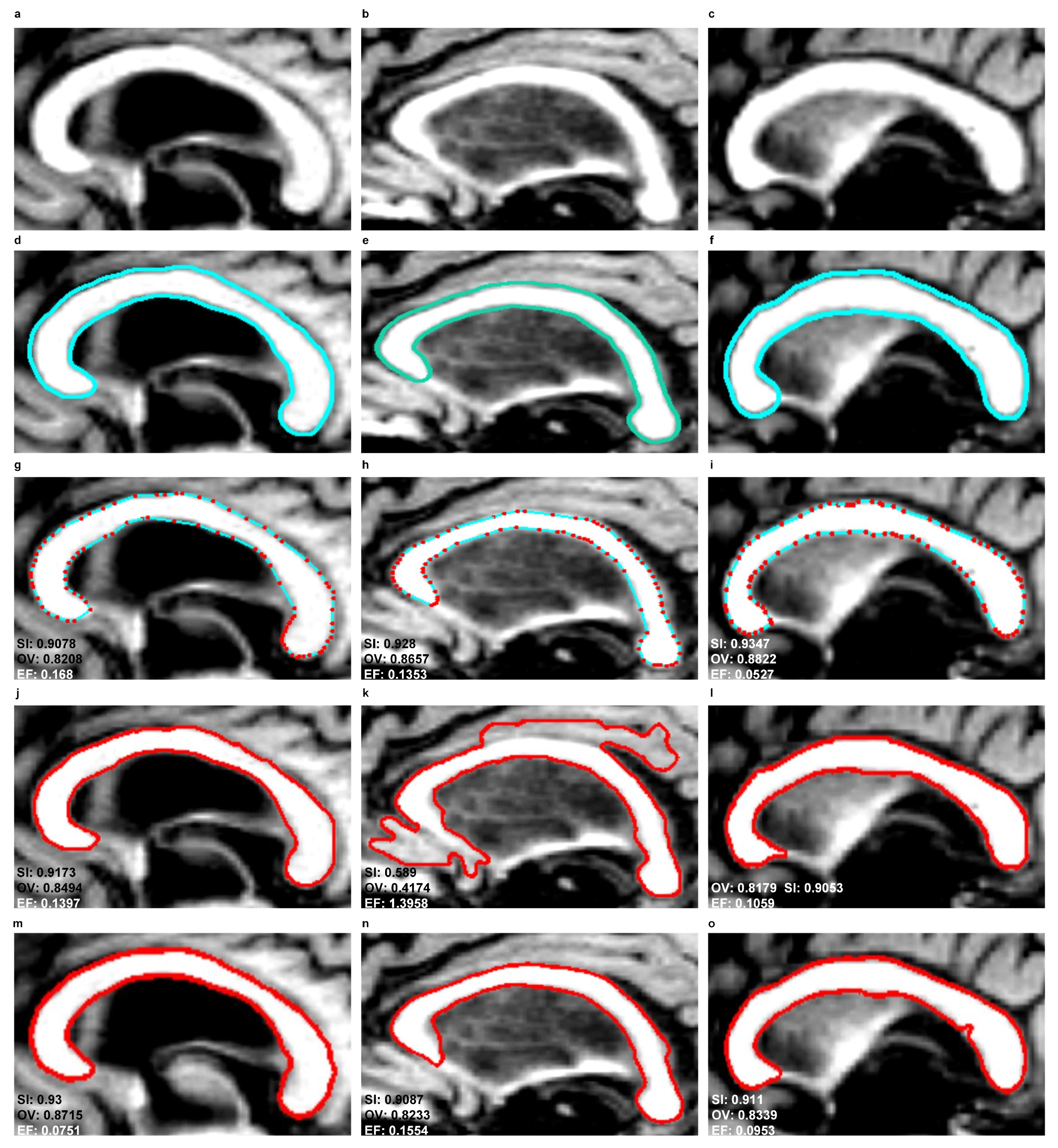
As a result of the experiments carried out, the EM model produced significantly better results of the mean SI (92%) and OV (85%) indices than SBGFRLS (SI = 82%, OV =72%) and DRLSE (SI = 73%, OV = 67%). Segmenting the CC using the DRLSE model may produce the greatest underestimation, as proven by the lowest minimum values of the $SI$ and $OV$ indices, which, for the DRLSE, amount to 41% and 28%, as also shown in examples from Figure 11m,o. The DRLSE and SBGFRLS models allow high segmentation results to be obtained for single CC slices, which has also been demonstrated in source articles [13,14]. However, if the entire set of CC slices is analysed as necessary to obtain an accurate 3D CC reconstruction, wrong segmentations (under- or over-segmentations) are produced for some images.

The average mean value of the $EF$ indice is the lowest for the DRLSE model and amounts to 9%. The EM and SBGFRLS models produced mean values of the EF indice amounting to 12% and 36% respectively, so if the SBGFRLS model is used, a very high over-segmentationmay occur.

Table 9. Summary of results of research on CC segmentation from MRIs for selected methods, based on a literature review. 2D means that the segmentation was carried out on the plane while 3D represents a 3D segmentation or performing a 3D reconstruction based on 2D cross-sections. [-] means that the article does not contain the respective information.

Method, Year	2D/3D, Modality	The Size of the Data Set Used to Calculate the SI and OV Indexes	Mean SI, OV	Tested Database
Pfefferbaum et al., [19], 2006	2D, 315, [-]	From 315 Patients	SI = 0.913	Control, HIV,
				Alcoholism
Adamson et al., [20], 2014	2D, T1	416 midsaggital slices	SI = 0. 887/0.875	Control,
				Alzheimer
Liu and Ruan [21], 2015	2D, [-]	100 midsaggital slices	SI = 0.95 ∓ 0.02	[-]
Bueno et al., [22], 2001	3D, T1	One phantom 3D MRI with provided ground truth.	Phatom 1 SI = 0.95, OV = 0.86	[-]
Karsch et al., [25], 2009	3D, [-]	16 slices	SI = 0.79 ∓ 0.05	[-]
Gass et al., [26], 2014	2D, [-]	70 midsaggital slices	SI = 0.935	Control
EM	2D/3D, T1	325 midsaggital slices	SI = 0.92 ∓ 0.015,	Alzheimer
			OV = 0.85 ∓ 0.035
SBGFRLS	2D/3D, T1	325 midsaggital slices	SI = 0.82 ∓ 0.14,	Alzheimer
			OV = 0.72 ∓ 0.192
DRLSE	2D/3D, T1	325 midsaggital slices	SI = 0.73 ∓ 0.211,	Alzheimer
			OV = 0.67 ∓ 0.223

presents the CC segmentation results measured by the SI and OV indices based on the results available in the literature. The results produced by the EM model are similar to the best results presented in publications [19,21,26]. In general, the larger the data set and the more measurements taken, the more difficult it is to obtain high values of the SI and OV indices.

Executing segmentations for complete sets of images containing CC cross-sections enabling the 3D reconstruction allows the utility of the methods applied to be assessed. This is particularly true as these sets also contain CC images with poorly visible edges. Segmenting only in single cross-sections [12,13,14] or in selected cross-sections with clearly visible edges means that the results obtained can be very high, e.g., in a previous study [12], the SI = 94% for 30 selected CC cross-sections taken from different sets of images.

Optimal parameters had been established before the experimental tests were conducted. This can be considered to constitute a certain limitation of the method presented. This is particularly so, because the EM model features as many as 10 parameters, of which four, i.e., ${\theta }_{min}$, ${\theta }_{max}$$D_{min}$ and $D_{max}$ control the number of nodes (automatically adding new ones and removing superfluous ones) and protect the active contour from the possible formation of self-crossings and loops. However, compared to the SBGFRLS and DRLSE models which have fewer parameters, the EM model produced significantly better segmentation results.

A key property of the EM model is the application of an inflation/deflation force together with node motion reversals and damping, which enables:

-

Initiation easier than in the DRLSE model [13], which can only increase or decrease its area. Conversely, the EM model can expand and shrink at the same time.

-

Restricting the undesirable phenomenon where the contour leaks outside the edges being approximated if they are indistinct. It is worth noting that, thanks to applying the pressure force, the SBGFRLS model has properties similar to the EM model, which improve its initialisation, since it can expand and shrink at the same time. However, the SBGFRLS model does not control the spillage of the contour beyond the edge approximated, and such spillage was abundant in it.

-

Using final contours for subsequent initiations to segment the CC. This approach simplifies the segmentation process. In comparable state-of-the-art models, i.e., DRLSE and SBGFRLS, the use of the final contours for subsequent initialisations was impossible because of certain limitations of these models presented above.

Furthermore, in the EM model, the nodes kept a high value of the inflation/deflation force and, if they did not reach the edge being identified, this allowed them to move efficiently. As a result, the maximum number of iterations is lower for the EM model than in the SBGFRLS and DRLSE ones.

5. Conclusions

This publication proposes a new method that allows segmenting the corpus callosum from MR images and then reconstructing it in 3D and visualising it. This all means that a tool that can aid the physician in their work was created using open source software systems.

The experimental tests and the summary of the research results support the claim that the use of the EM model allowed better CC segmentation and 3D visualisation results to be produced than the use of the DRLSE and SBGFRLS models, and the segmentation results are similar to or better than of other methods ascertained from the literature review. Detailed research carried out as part of this research project and the discussion of the advantages and limitations of the active contour models used can be useful for proposing further new solutions.

In future research, the methods presented in this study will be assessed on a large set of patient data, also those suffering from other conditions, like the human immunodeficiency virus (HIV), autism or alcoholism. The approach presented here can also be extended and adapted to segmenting other organs, e.g., the carotid and vertebral arteries in CT angiography (CTA).

References

- Shen, P.; Li, C. Local feature extraction and information bottleneck-based segmentation of brain magnetic resonance (mr) images. Entropy 2013, 15, 3205–3218. [Google Scholar] [CrossRef]
- Ji, Z.; Liu, J.; Cao, G.; Sun, Q.; Chen, Q. Robust spatially constrained fuzzy c-means algorithm for brain MR image segmentation. Pattern Recognit. 2014, 47, 2454–2466. [Google Scholar] [CrossRef]
- Tu, X.; Gao, J.; Zhu, C.; Cheng, J.Z.; Ma, Z.; Dai, X.; Xie, M. MR image segmentation and bias field estimation based on coherent local intensity clustering with total variation regularization. Med. Biol. Eng. Comput. 2016, 54, 1807–1818. [Google Scholar] [CrossRef] [PubMed]
- Wang, S.; Lu, S.; Dong, Z.; Yang, J.; Yang, M.; Zhang, Y. Dual-tree complex wavelet transform and twin support vector machine for pathological brain detection. Appl. Sci. 2016, 6, 169. [Google Scholar] [CrossRef]
- Davarpanah, S.H.; Liew, A.W.C. Spatial possibilistic Fuzzy C-Mean segmentation algorithm integrated with brain mid-sagittal surface information. Int. J. Fuzzy Syst. 2017, 19, 591–605. [Google Scholar] [CrossRef]
- Namburu, A.; kumar Samay, S.; Edara, S.R. Soft fuzzy rough set-based MR brain image segmentation. Appl. Soft Comput. 2017, 54, 456–466. [Google Scholar] [CrossRef]
- Wang, S.H.; Cheng, H.; Phillips, P.; Zhang, Y.D. Multiple Sclerosis Identification Based on Fractional Fourier Entropy and a Modified Jaya Algorithm. Entropy 2018, 20, 254. [Google Scholar] [CrossRef]
- Hofer, S.; Frahm, J. Topography of the human corpus callosum revisited–comprehensive fiber tractography using diffusion tensor magnetic resonance imaging. Neuroimage 2006, 32, 989–994. [Google Scholar] [CrossRef] [PubMed]
- Radanovic, M.; Pereira, F.R.S.; Stella, F.; Aprahamian, I.; Ferreira, L.K.; Forlenza, O.V.; Busatto, G.F. White matter abnormalities associated with Alzheimer’s disease and mild cognitive impairment: A critical review of MRI studies. Expert Rev. Neurother. 2013, 13, 483–493. [Google Scholar] [CrossRef] [PubMed]
- Ozturk, A.; Smith, S.; Gordon-Lipkin, E.; Harrison, D.; Shiee, N.; Pham, D.; Caffo, B.; Calabresi, P.; Reich, D. MRI of the corpus callosum in multiple sclerosis: association with disability. Mult. Scler. J. 2010, 16, 166–177. [Google Scholar] [CrossRef] [PubMed] [Green Version]
- Malone, I.B.; Cash, D.; Ridgway, G.R.; MacManus, D.G.; Ourselin, S.; Fox, N.C.; Schott, J.M. MIRIAD–Public release of a multiple time point Alzheimer’s MR imaging dataset. NeuroImage 2013, 70, 33–36. [Google Scholar] [CrossRef] [PubMed]
- Ciecholewski, M. An edge-based active contour model using an inflation/deflation force with a damping coefficient. Expert Syst. Appl. 2016, 44, 22–36. [Google Scholar] [CrossRef]
- Li, C.; Xu, C.; Gui, C.; Fox, M.D. Distance regularized level set evolution and its application to image segmentation. IEEE Trans. Image Process. 2010, 19, 32–43. [Google Scholar]
- Zhang, K.; Zhang, L.; Song, H.; Zhou, W. Active contours with selective local or global segmentation: A new formulation and level set method. Image Vis. Comput. 2010, 28, 668–676. [Google Scholar] [CrossRef]
- Ciecholewski, M. Malignant and Benign Mass Segmentation in Mammograms Using Active Contour Methods. Symmetry 2017, 9, 277. [Google Scholar] [CrossRef]
- Consortium, I.S. Itk: Insight Segmentation and Registration Toolkit. 2011. Available online: http://www.itk.org/ (accessed on 23 November 2011).
- Schroeder, W.J.; Lorensen, B.; Martin, K. Vtk–the visualization toolkit. Kitware, 2011. Available online: http://www.vtk.org/ (accessed on 25 November 2011).
- Yushkevich, P.A.; Piven, J.; Hazlett, H.C.; Smith, R.G.; Ho, S.; Gee, J.C.; Gerig, G. User–guided 3D active contour segmentation of anatomical structures: significantly improved efficiency and reliability. Neuroimage 2006, 31, 1116–1128. [Google Scholar] [CrossRef] [PubMed]
- Pfefferbaum, A.; Rosenbloom, M.J.; Rohlfing, T.; Adalsteinsson, E.; Kemper, C.A.; Deresinski, S.; Sullivan, E.V. Contribution of alcoholism to brain dysmorphology in HIV infection: effects on the ventricles and corpus callosum. Neuroimage 2006, 33, 239–251. [Google Scholar] [CrossRef] [PubMed]
- Adamson, C.; Beare, R.; Walterfang, M.; Seal, M. Software pipeline for midsagittal corpus callosum thickness profile processing. Neuroinformatics 2014, 12, 595–614. [Google Scholar] [CrossRef] [PubMed]
- Liu, W.; Ruan, D. A unified variational segmentation framework with a level-set based sparse composite shape prior. Phys. Med. Biol. 2015, 60, 1865. [Google Scholar] [CrossRef] [PubMed]
- Bueno, G.; Musse, O.; Heitz, F.; Armspach, J. Three–dimensional segmentation of anatomical structures in MR images on large data bases. Magn. Reson. Imaging 2001, 19, 73–88. [Google Scholar] [CrossRef]
- El-Baz, A.; Elnakib, A.; Casanova, M.F.; Gimel’farb, G.; Switala, A.E.; Jordan, D.; Rainey, S. Accurate automated detection of autism related corpus callosum abnormalities. J. Med. Syst. 2011, 35, 929–939. [Google Scholar] [CrossRef] [PubMed]
- Xu, J.; Liang, F.; Gu, L. Bayesian co-segmentation of multiple MR images. In Proceedings of the 2009 IEEE International Symposium on Biomedical Imaging: From Nano to Macro, Boston, MA, USA, 28 June–1 July 2009; pp. 53–56. [Google Scholar]
- Karsch, K.; He, Q.; Duan, Y. A fast, semi-automatic brain structure segmentation algorithm for magnetic resonance imaging. In Proceedings of the IEEE International Conference on Bioinformatics and Biomedicine, BIBM’09, Washington, DC, USA, 1–4 November 2009; pp. 297–302. [Google Scholar]
- Gass, T.; Szekely, G.; Goksel, O. Simultaneous segmentation and multiresolution nonrigid atlas registration. IEEE Trans. Image Process. 2014, 23, 2931–2943. [Google Scholar] [CrossRef] [PubMed]
- Vincent, L.; Soille, P. Watersheds in digital spaces: An efficient algorithm based on immersion simulations. EEE Trans. Pattern Anal. Mach. Intell. 1991, 13, 583–598. [Google Scholar] [CrossRef]
- Cover, G.; Herrera, W.; Bento, M.; Appenzeller, S.; Rittner, L. Computational methods for corpus callosum segmentation on MRI: A systematic literature review. Comput. Methods Programs Biomed. 2018, 154, 25–35. [Google Scholar] [CrossRef] [PubMed]
- Lorensen, W.E.; Cline, H.E. Marching cubes: A high resolution 3D surface construction algorithm. In ACM Siggraph Computer Graphics; ACM: New York, NY, USA, 1987; Volume 21, pp. 163–169. [Google Scholar]
- Crawford, C.R.; Cline, H.E.; Lorensen, W.E.; Teeter, B.C. 3–d imaging using normalized gradient shading in ct and mri. In Medical Imaging III: Image Capture and Display; SPIE—The International Society for Optical Engineering: Bellingham, WA, USA, 1989; Volume 1091, pp. 294–301. [Google Scholar]
- Gonzales, R.; Woods, E. Digital Image Processing, 3rd ed.; Prentice-Hall, Inc.: Upper Saddle River, NJ, USA, 2007. [Google Scholar]
- Bosma, M. Iso-surface Volume Rendering: Speed and Accuracy for Medical Applications, Ph.D. Thesis, University of Twente, Enschede, The Netherland, 2000. [Google Scholar]
- Carr, J.C.; Beatson, R.K.; Cherrie, J.B.; Mitchell, T.J.; Fright, W.R.; McCallum, B.C.; Evans, T.R. Reconstruction and representation of 3D objects with radial basis functions. In Proceedings of the 28th Annual Conference on Computer Graphics and Interactive Techniques, Los Angeles, CA, USA, 12–17 August 2001; ACM: New York, NY, USA, 2001; pp. 67–76. [Google Scholar] [Green Version]
- Carr, J.C.; Beatson, R.K.; McCallum, B.C.; Fright, W.R.; McLennan, T.J.; Mitchell, T.J. Smooth surface reconstruction from noisy range data. In Proceedings of the 1st International Conference on Computer Graphics and Interactive Techniques in Australasia and South East Asia, Singapore, 15–18 June 2004; ACM: New York, NY, USA; pp. 119–126. [Google Scholar]
Figure 1.
The Corpus Callosum (CC) in an example midsagittal brain Magnetic Resonance (MR) image. Data source: Minimal Interval Resonance Imaging in Alzheimer’s Disease (MIRIAD) [11], from the ’miriad_188_1_MR_1’ set.
Figure 2.
The proposed approach to segmenting the corpus callosum (CC), reconstructing it and visualising it in 3D based on brain MR images.
Figure 3.
A diagram of segmenting the corpus callosum in a midsaggital plane of a brain MRI using active contour methods, namely: an edge-based active contour model using an inflation/deflation force with a damping coefficient (EM), Distance Regularized Level Set Evolution (DRLSE) method, Selective Binary and Gaussian Filtering Regularized Level Set (SBGFRLS) method.
Figure 4.
Corpus callosum segmentation using an EM model, from an image in the midsaggital plane from the set ’miriad_188_1_MR_1’. (a) a rectangular seed contour made up of four nodes; (b) the final contour produced using Equation (8) and solutions presented in study [12]; (c) a graph based on an experiment for which the final contour is presented under (b). In addition, 900 iterations were set, during which the maximum number of nodes amounted to 378, and the processing time was: 236.8 s. (Time was measured on a personal computer with an Intel Core i7-2630QM CPU @ 2 GHz and 16 GB of RAM under the Windows 10 platform); (d) the final contour produced by Algorithm 1; (e) a graph based on an experiment for which the final contour is presented under (d). 350 iterations were set, during which the maximum number of nodes amounted to 127, and the processing time was: 67.8 s.
Figure 5.
Using the ITK–SNAP platform to visualise the CC. (a–c) displaying axial, sagittal and coronal planes; (d) 3D visualization of segmented CC.
Figure 6.
Preprocessing an example image from the ’miriad_188_1_MR_1’ set. (a) unprocessed source image; (b) processed image with contrast strengthened.
Figure 7.
An example illustrating the results of corpus callosum segmentation using the EM, DRLSE and SBGFRLS methods for two different contour initialisations—A and B–based on an MR image in the sagittal plane from the ’miriad_188_AD_M_01_MR_1’ set (a) a contour traced by a physician (); (b) a rectangular seed contour: A; (c–e) final contours produced by the EM, DRLSE and SBGFRLS methods with initialisation A; (f) a rectangular seed contour: B; (g–i) final contours produced by the EM, DRLSE and SBGFRLS methods with initialisation B.
Figure 8.
Corpus callosum segmentation from subsequent example MR images in the sagittal plane, taken from the ’miriad_188_1_MR_1’ set. Row one: ROIs of corpus callosum images taken from three subsequent sagittal planes. Row two: Contours produced by the EM model. Row three: use of the SBGFRLS model. Row four: the DRLSE model. (a) ROI from the first image; (b) ROI from the second image; (c) ROI from the third image; (d) final contour produced based on the contour from item; (e) after 20 iterations were completed; (e) final contour from Figure 7g produced using the initialisation presented in Figure 7f by executing 400 iterations; (f) final contour produced based on the contour from item; (e) after 20 iterations were completed; (g–i) final contours produced based on images from items (a–c) after completing 550 iterations, with the same initialisation from Figure 7f; (j–l) final contours produced based on images from items (a–c) after completing 875 iterations, with the same initialisation from Figure 7f.
Figure 9.
Graphs of the mean value and the standard deviation based on measurements of three indices—SI, OV, EF—for the three applied methods—EM, SBGFRLS and DRLSE—compared to the contours traced by the physician (Expert) based on data from Table 8.
Figure 10.
Comparison of corpus callosum segmentation results for example MR images taken from three sets from the MIRIAD database. First column: ‘miriad_189_AD_M_05_MR_1’, second column: ‘miriad_190_AD_M_02_MR_1’, third column: ‘miriad_205_AD_F_05_MR_1’. First row: ROIs from MR images of the corpus callosum based on the sagittal plane, Second row: contours traced by a physician (), Third row: contours produced by the EM model, Fourth row: use of the SBGFRLS model, Fifth row: the DRLSE model.
Figure 11.
Comparison of corpus callosum segmentation results for example MR images taken from three sets from the MIRIAD database. First column: ‘miriad_234_AD_M_03_MR_2’, second column: ‘miriad_244_AD_F_01_MR_2’, third column: ‘miriad_257_AD_F_05_MR_1’. First row: ROIs from MR images of the corpus callosum based on the sagittal plane, Second row: contours traced by a physician (), Third row: contours produced by the EM model, Fourth row: use of the SBGFRLS model, Fifth row: the DRLSE model.
Figure 12.
3D CC models (sagittal view) based on the segmentations produced and the subsequent 3D reconstruction. First column: ‘miriad_234_AD_M_03_MR_2’, second column: ‘miriad_244_AD_F_01_MR_2’, third column: ‘miriad_257_AD_F_05_MR_1’. First row: a model produced based on a segmentation manually traced by a physician (), Second row: with EM; Third row: with DRLSE. Fourth row: SBGFRLS.
Figure 13.
Inverted 3D CC models, continued from Figure 12.