Constraints on Lorentz Invariance Violation from Optical Polarimetry of Astrophysical Objects

Abstract
1. Introduction
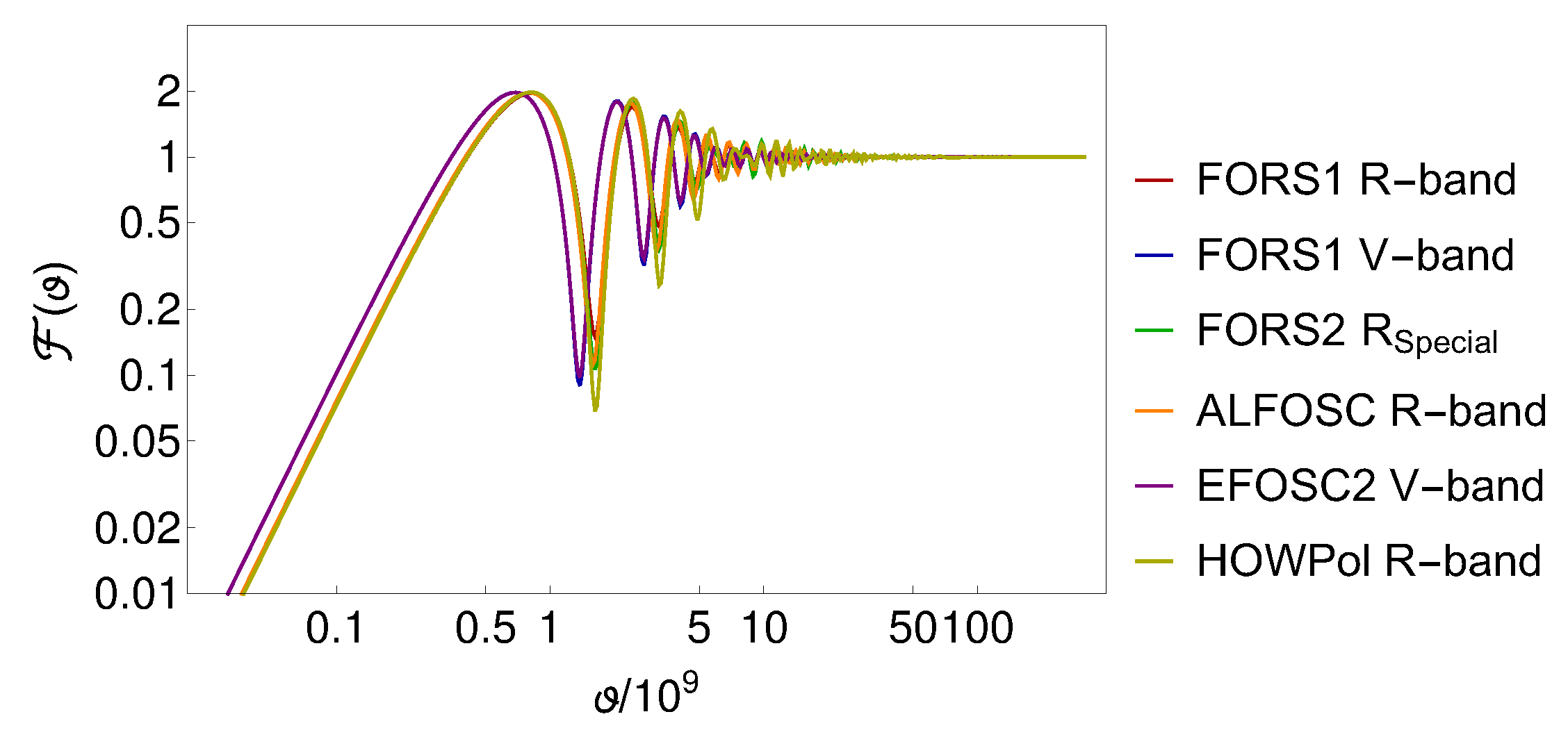
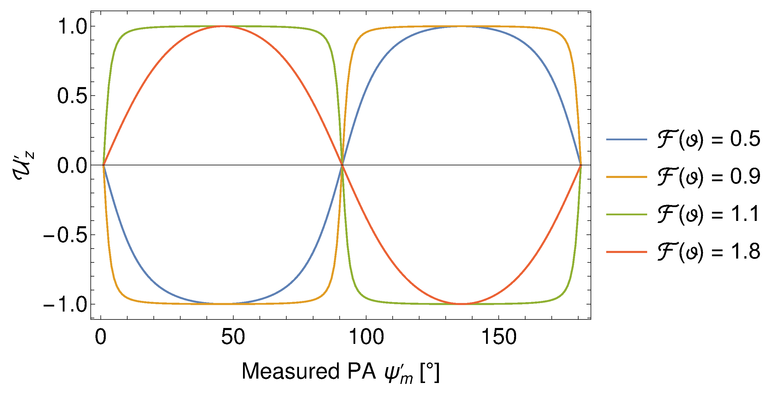
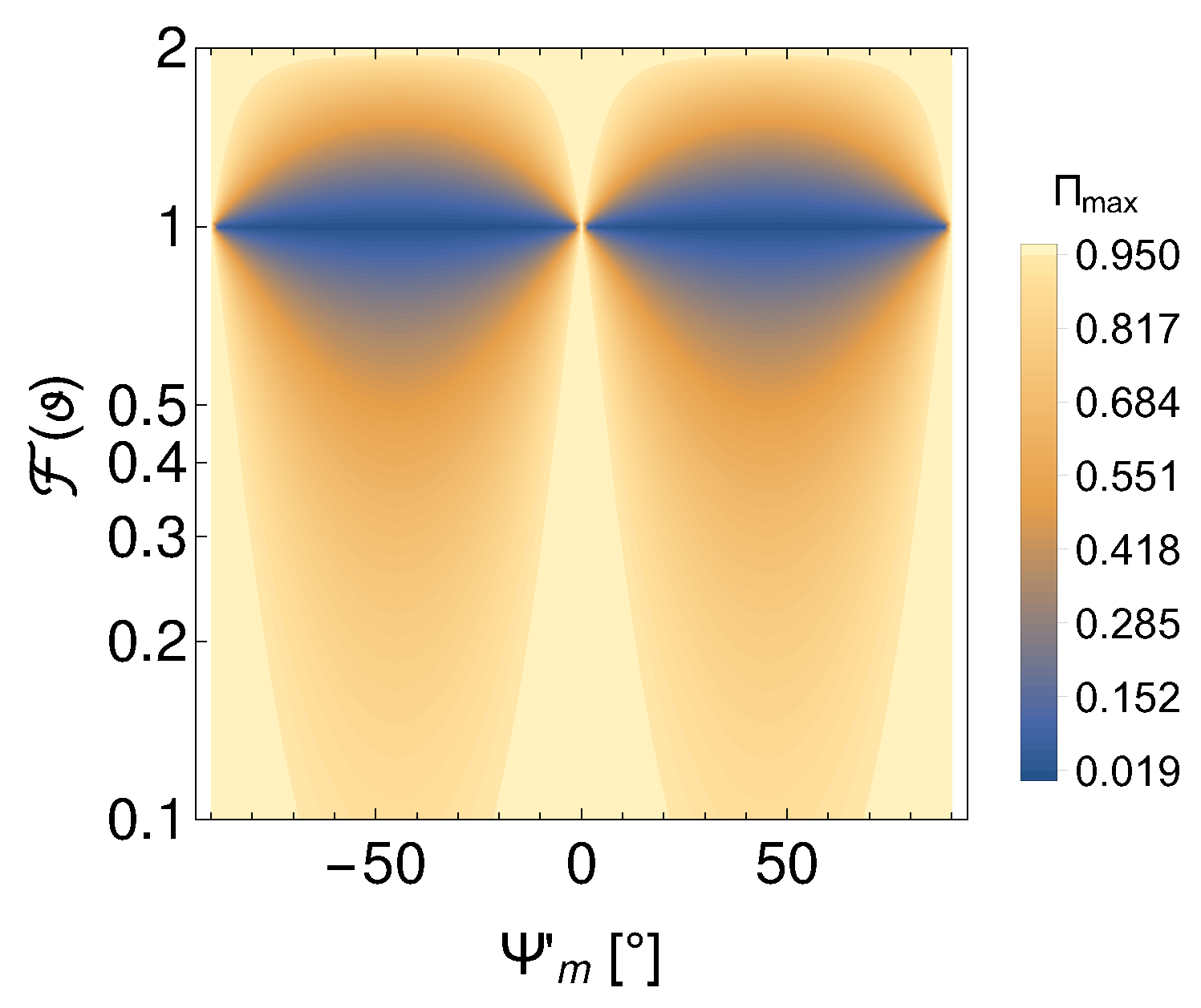
2. Theory
3. Astrophysical Polarization Measurements
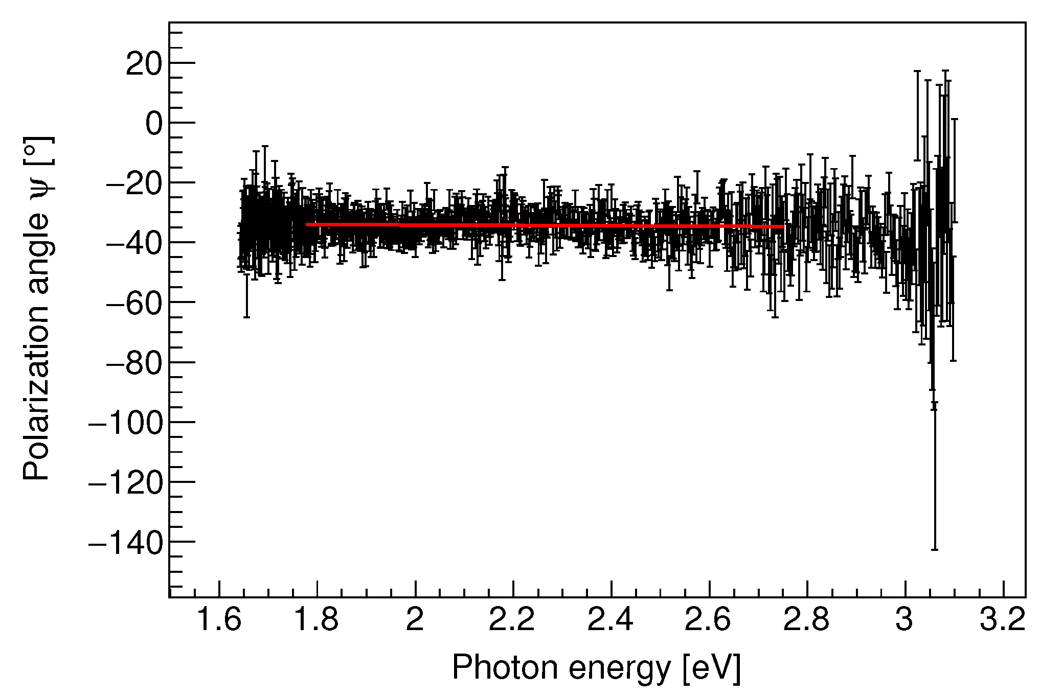
3.1. Spectropolarimetry
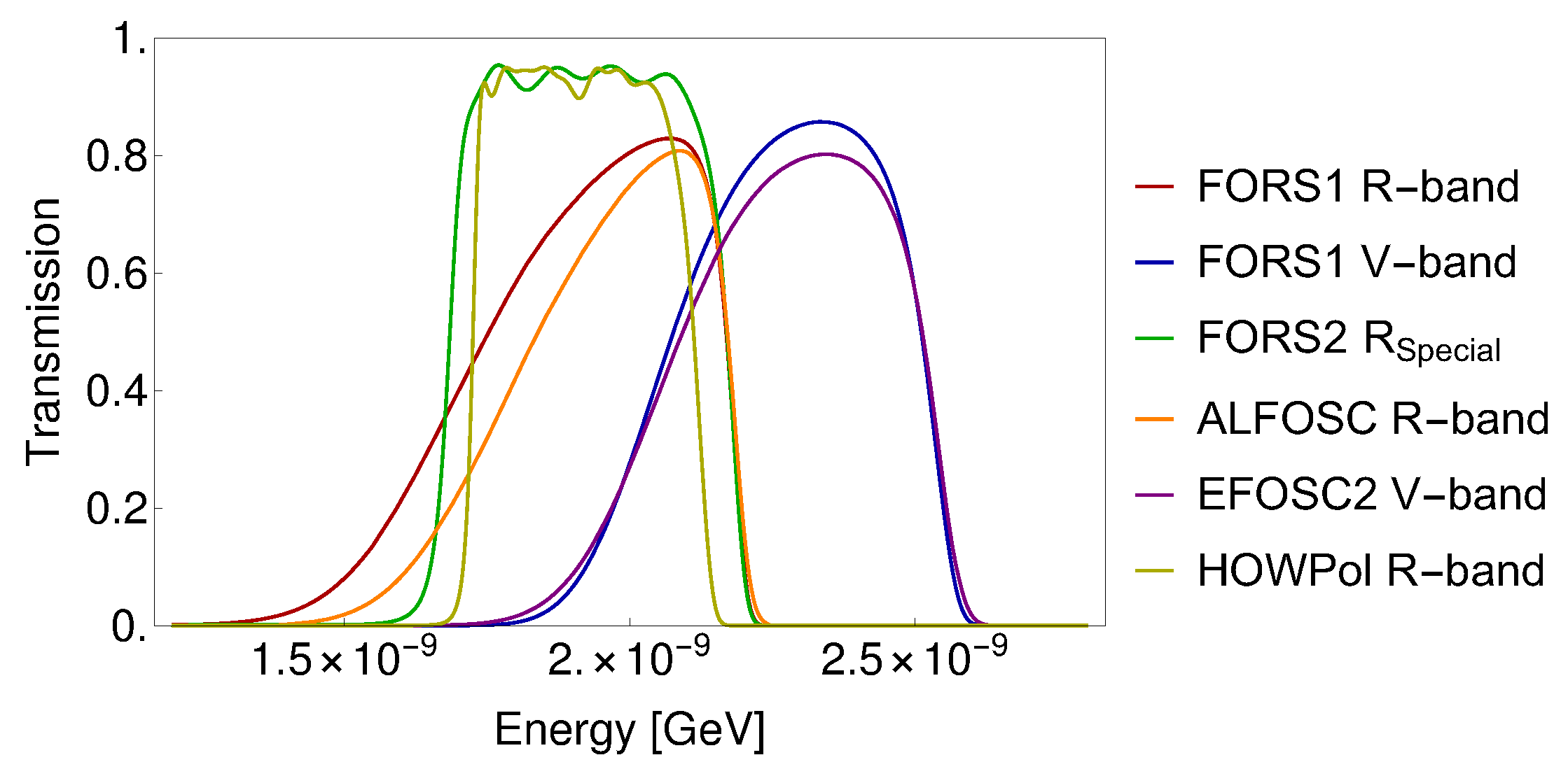
3.2. Polarimetry Integrated over a Broad Bandwidth
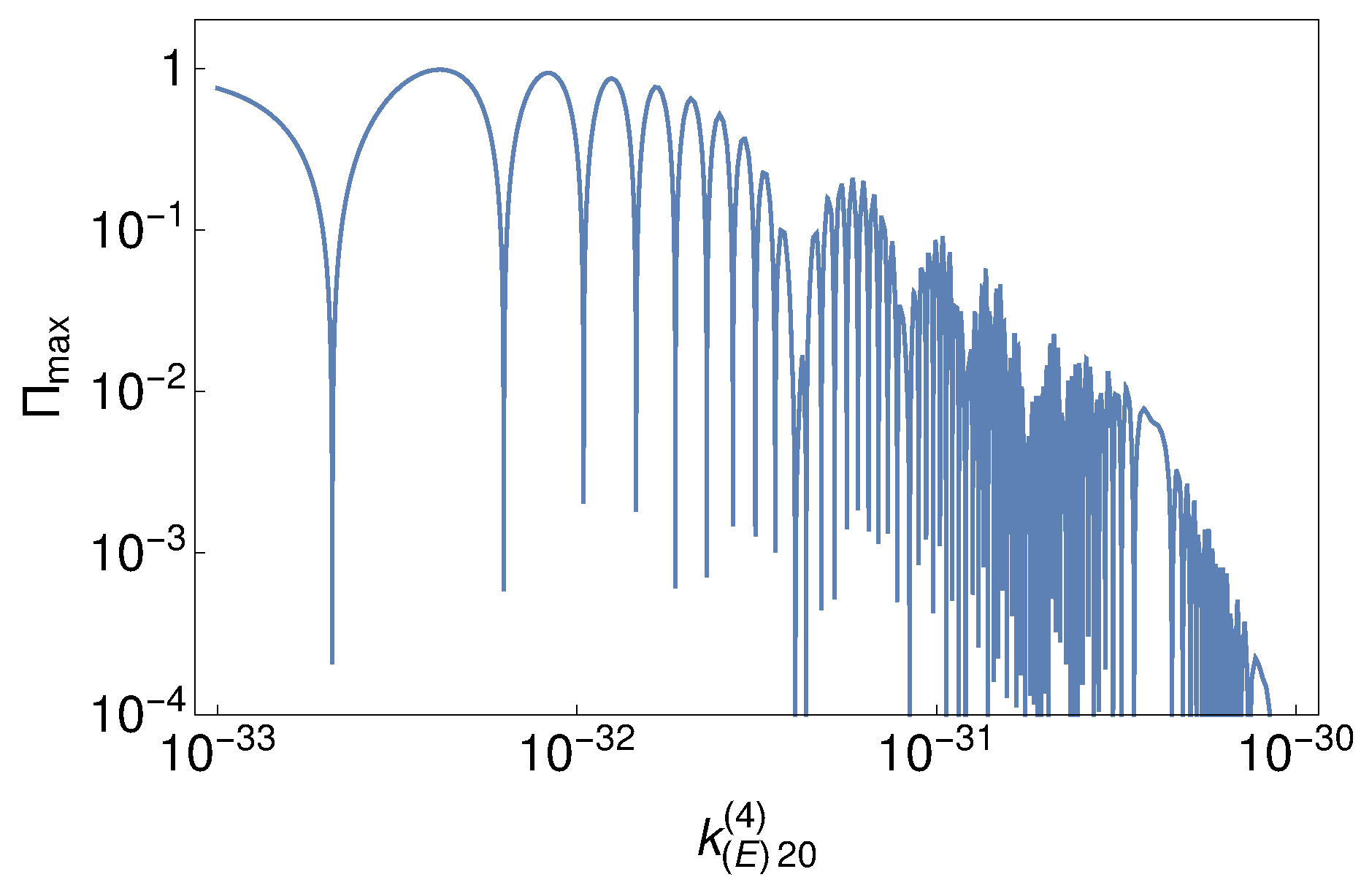
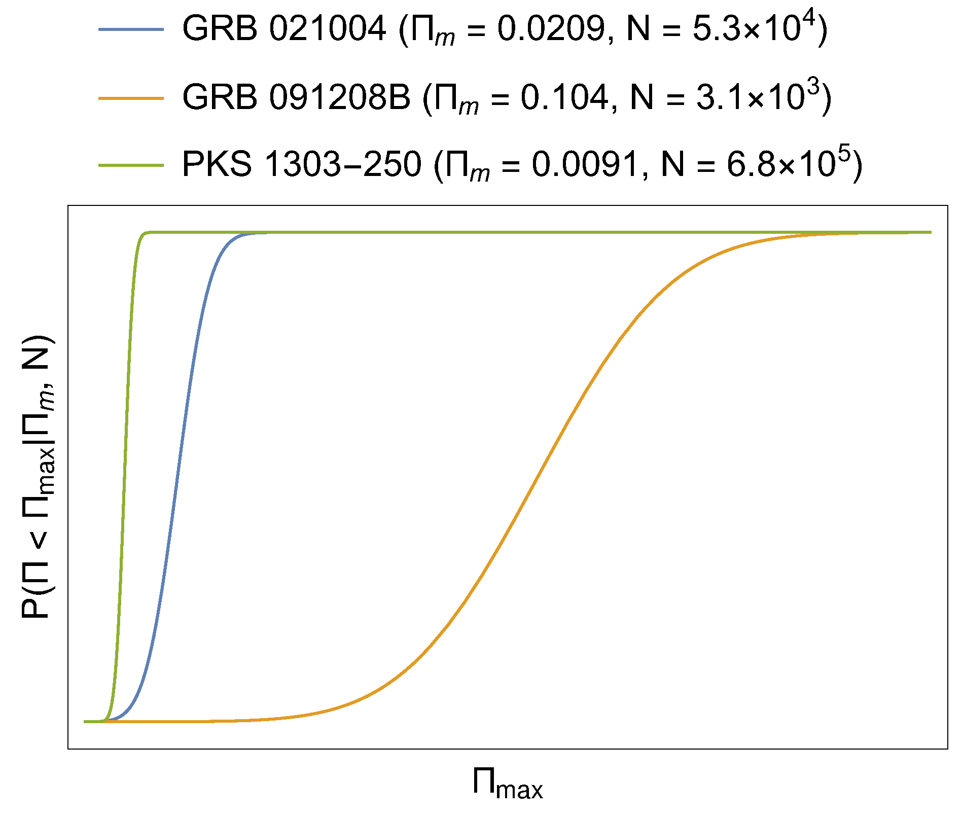
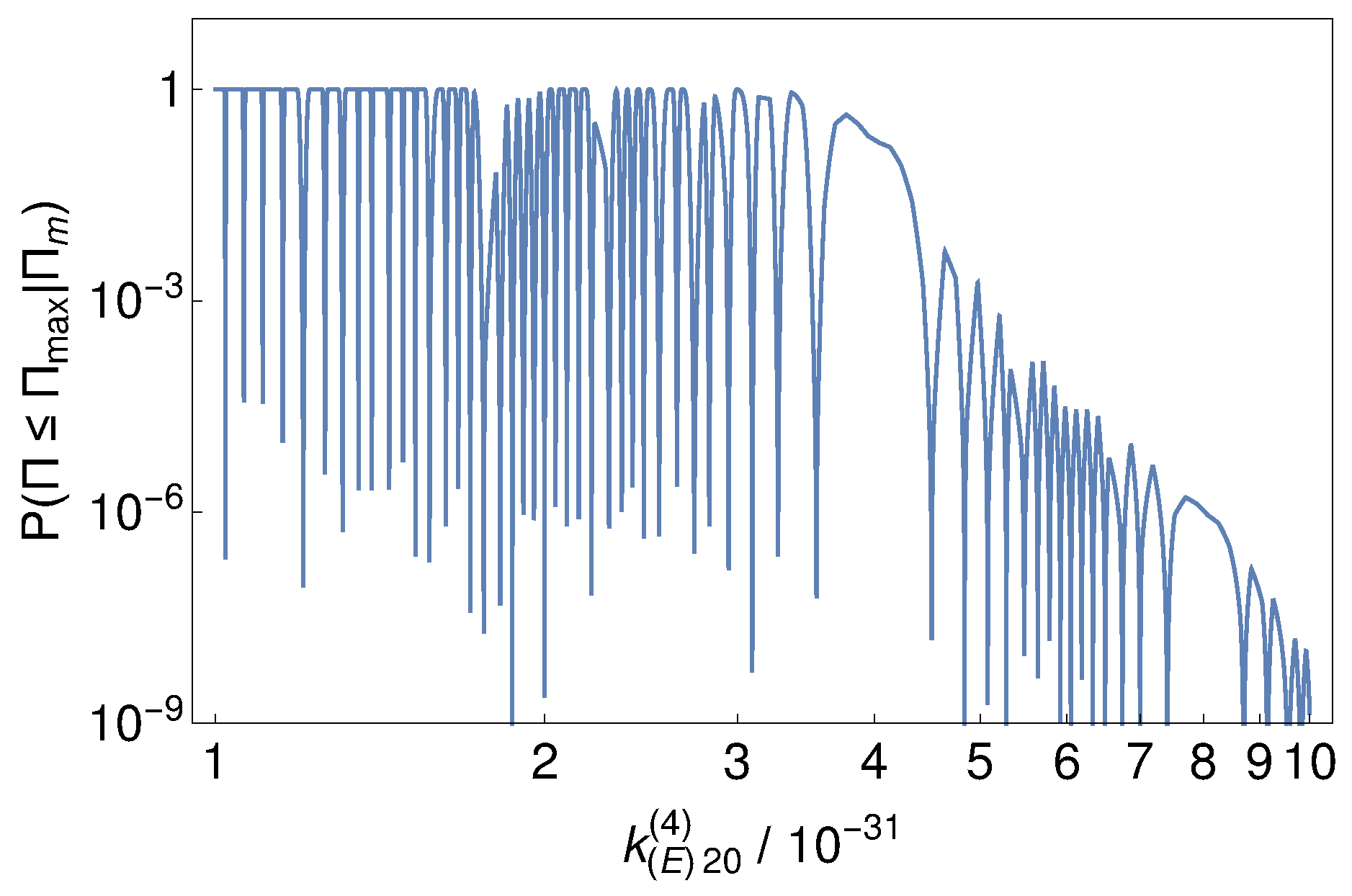
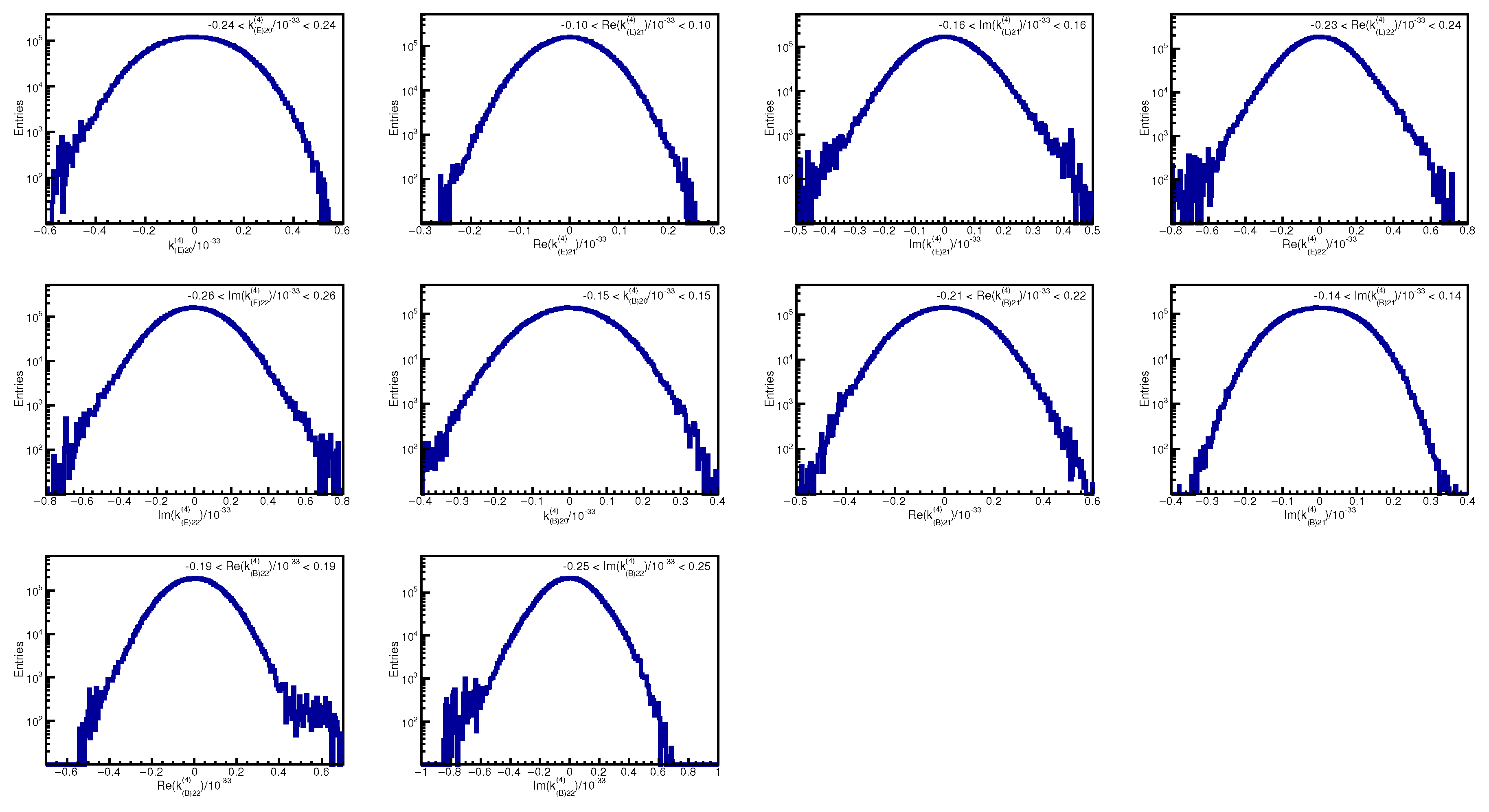
4. Results
5. Discussion
Funding
Acknowledgments
Conflicts of Interest
Appendix A. Astrophysical Sources

| Source | RA J2000 [] | Dec. J2000 [] | Redshift z | Polarization [%] | Position Angle [] |
|---|---|---|---|---|---|
| SDSS J0242+0049 | 40.591 | +0.820 | 2.071 | 1.47(24) | −13(5) |
| FIRST03133+0036 | 48.328 | +0.606 | 1.250 | 1.48(29) | −55(6) |
| FIRST J0809+2753 | 122.256 | +27.895 | 1.511 | 1.75(20) | 73(3) |
| PG 0946+301 | 147.421 | +29.922 | 1.220 | 1.65(19) | −66(3) |
| PKS 1124−186 | 171.768 | −17.045 | 1.048 | 11.68(36) | 37(1) |
| He 1127−1304 | 172.583 | −12.653 | 0.634 | 1.32(13) | 46(3) |
| 2QZ J114954+0012 | 177.479 | +0.215 | 1.596 | 1.57(22) | −24(4) |
| SDSS J1206+0023 | 181.615 | +0.393 | 2.331 | 0.94(15) | −57(5) |
| SDSS J1214−0001 | 183.673 | +0.027 | 1.041 | 2.40(32) | −77(4) |
| PKS 1219+04 | 185.594 | +4.221 | 0.965 | 5.56(15) | −61(1) |
| PKS 1222+037 | 186.218 | +3.514 | 0.960 | 2.51(22) | −82(2) |
| TON 1530 | 186.364 | +22.587 | 2.058 | 0.92(14) | −11(4) |
| SDSS J1234+0057 | 188.616 | +0.966 | 1.532 | 1.35(23) | 2(5) |
| PG 1254+047 | 194.250 | +4.459 | 1.018 | 0.84(15) | −4(5) |
| PKS 1256−229 | 194.785 | −22.823 | 1.365 | 22.32(15) | −23(1) |
| SDSS J1302−0037 | 195.534 | +0.626 | 1.672 | 1.37(20) | 35(4) |
| PKS 1303−250 | 196.564 | −24.711 | 0.738 | 0.91(17) | −75(5) |
| FIRST J1312+2319 | 198.056 | +23.333 | 1.508 | 1.10(16) | −14(4) |
| SDSS J1323−0038 | 200.769 | +0.649 | 1.827 | 1.13(21) | 15(5) |
| CTS J13.07 | 205.518 | −17.700 | 2.210 | 0.83(15) | 20(5) |
| SDSS J1409+0048 | 212.328 | +0.807 | 1.999 | 3.91(28) | 30(2) |
| HS 1417+2547 | 215.055 | +25.568 | 2.200 | 1.03(18) | −66(5) |
| FIRST J1427+2709 | 216.765 | +27.161 | 1.170 | 1.35(25) | 80(5) |
| FIRST J21079−0620 | 316.990 | −5.664 | 0.644 | 1.12(22) | −33(6) |
| SDSS J2131−0700 | 322.912 | −6.996 | 2.048 | 1.78(32) | 44(5) |
| PKS 2204−54 | 331.932 | −52.224 | 1.206 | 1.81(26) | −50(4) |
| PKS 2227−445 | 337.735 | −43.725 | 1.326 | 5.26(48) | 18(3) |
| PKS 2240−260 | 340.860 | −24.258 | 0.774 | 14.78(21) | −49(1) |
| PKS 2301+06 | 346.118 | +6.336 | 1.268 | 3.69(26) | −17(2) |
| SDSS J2319−0024 | 349.995 | +0.414 | 1.889 | 1.85(30) | −16(5) |
| PKS 2320−035 | 350.883 | −2.715 | 1.411 | 9.56(20) | 90(1) |
| PKS 2332−017 | 353.835 | −0.481 | 1.184 | 4.86(19) | −88(1) |
| PKS 2335−027 | 354.489 | −1.484 | 1.072 | 3.55(30) | −70(2) |
| SDSS J2352+0105 | 358.159 | +1.098 | 2.156 | 1.59(26) | 27(5) |
| SDSS J2356−0036 | 359.120 | +0.601 | 2.936 | 1.81(34) | 16(5) |
| QSO J2359−12 | 359.973 | −11.303 | 0.868 | 4.12(20) | −29(1) |
| Source | Instrument | RA | Dec. | Redshift | Polarization | Position Angle | Refs. |
|---|---|---|---|---|---|---|---|
| J2000 [] | J2000 [] | z | [%] | [] | |||
| GRB 990510 | FORS1 R−band | 204.532 | −80.497 | 1.619 | 1.6(2) | −84(4) | [41,42,43] |
| GRB 990712 | FORS1 R-band | 337.971 | −73.408 | 0.430 | 2.9(4) | −59(4) | [44] |
| GRB 020813 | FORS1 V-band | 296.674 | −19.601 | 1.25 | 1.42(25) | −43(4) | [47,48] |
| GRB 021004 | NOT/ALFOSC | 6.728 | +18.928 | 2.330 | 2.1(6) | −7(8) | [45] |
| GRB 030329 | NOT/ALFOSC | 161.208 | +21.522 | 0.169 | 2.4(4) | 65(7) | [46] |
| GRB 091018 | FORS2 | 32.192 | −57.55 | 0.97 | 3.25(35) | 57(6) | [49] |
| GRB 091208B | HOWPol | 29.410 | 16.881 | 1.06 | 10.4(25) | −88(6) | [50] |
| GRB 121024A | FORS2 | 70.467 | −12.268 | 2.298 | 4.83(20) | 173 | [51] |
| Source | RA | Dec. | Redshift | PA at 2.26 eV | |||
|---|---|---|---|---|---|---|---|
| [%] | J2000 [] | J2000 [] | z | [] | [] | ||
| 3C 454.3 | 18.83 | 343.491 | +16.148 | 0.859 | [60] | 61.19(23) | −0.3(10) |
| 4C 14.23 | 20.32 | 111.320 | +14.420 | 1.038 | [61] | −34.42(18) | −0.7(7) |
| 4C 28.07 | 30.30 | 39.468 | +28.802 | 1.206 | [61] | −62.36(9) | 0.46(32) |
| AO 0235+164 | 39.79 | 39.662 | +16.616 | 0.940 | [62] | −20.25(5) | 0.16(17) |
| B2 1633+382 | 27.26 | 248.815 | +38.135 | 1.813 | [63] | −3.71(7) | −0.69(26) |
| B2 1846+32A | 28.88 | 282.092 | +32.317 | 0.800 | [61] | 2.39(5) | 1.49(18) |
| B3 0650+453 | 16.16 | 103.599 | +45.240 | 0.928 | [61] | 79.3(5) | 3.4(18) |
| B3 1343+451 | 10.07 | 206.388 | +44.883 | 2.534 | [61] | 35.6(6) | −0.7(26) |
| BZU J0742+5444 | 21.73 | 115.666 | +54.740 | 0.723 | [64] | −87.84(19) | 2.2(6) |
| CTA 26 | 26.21 | 54.879 | −1.777 | 0.852 | [65] | 67.49(7) | −0.13(24) |
| CTA 102 | 23.97 | 338.152 | +11.731 | 1.037 | [66] | 64.81(9) | 1.29(34) |
| MG1 J123931+0443 | 33.61 | 189.886 | +4.718 | 1.760 | [63] | −72.28(8) | −0.02(32) |
| OJ 248 | 18.09 | 127.717 | +24.183 | 0.941 | [63] | −79.23(11) | −0.9(4) |
| PKS 0420−014 | 28.67 | 65.816 | −1.343 | 0.916 | [67] | 10.23(9) | 0.44(31) |
| PKS 0454-234 | 35.27 | 74.263 | −23.414 | 1.003 | [60] | 2.49(6) | 0.22(20) |
| PKS 0502+049 | 17.59 | 76.347 | +4.995 | 0.954 | [68] | −87.82(13) | 2.1(5) |
| PKS 0805−077 | 28.27 | 122.065 | −7.853 | 1.837 | [60] | 41.7(4) | −1.4(11) |
| PKS 1118−056 | 22.54 | 170.355 | −5.899 | 1.297 | [60] | 37.26(9) | 1.4(7) |
| PKS 1124-186 | 10.49 | 171.768 | −18.955 | 1.048 | [62] | −83.18(19) | 0.2(7) |
| PKS 1244−255 | 13.97 | 191.695 | −25.797 | 0.638 | [60] | −14.07(11) | 1.9(4) |
| PKS 1441+252 | 37.70 | 220.987 | +25.029 | 0.939 | [61] | −72.34(8) | 0.51(28) |
| PKS 1502+106 | 45.16 | 226.104 | +10.494 | 1.839 | [63] | 65.43(12) | 0.1(4) |
| PKS 2032+107 | 12.36 | 308.843 | +10.935 | 0.601 | [61] | 68.4(10) | 9.2(34) |
| PMN J2345-1555 | 32.69 | 356.302 | −15.919 | 0.621 | [61] | −0.46(4) | 1.30(15) |
| S4 1030+61 | 37.71 | 158.464 | +60.852 | 1.400 | [63] | −59.69(12) | −1.3(4) |
| SDSS J084411+5312 | 18.72 | 131.049 | +53.214 | 3.704 | [63] | 8.4(4) | −2.0(17) |
| Ton 599 | 33.16 | 179.883 | +29.246 | 0.724 | [63] | −52.69(7) | 0.86(26) |
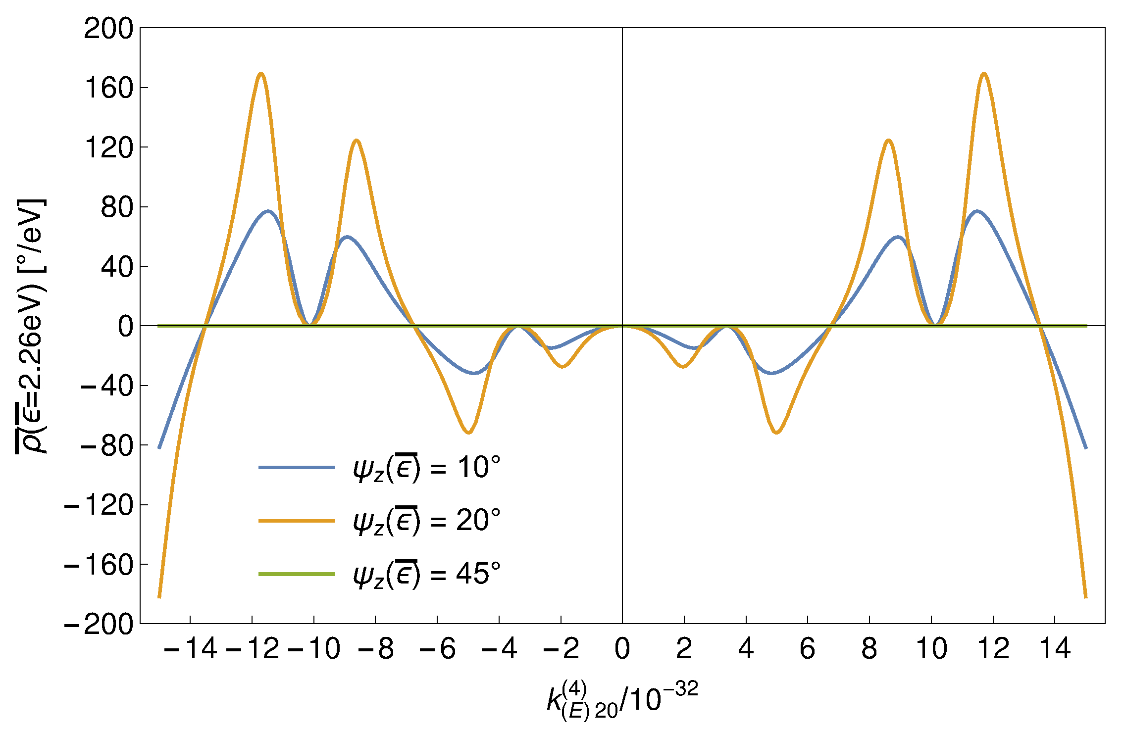
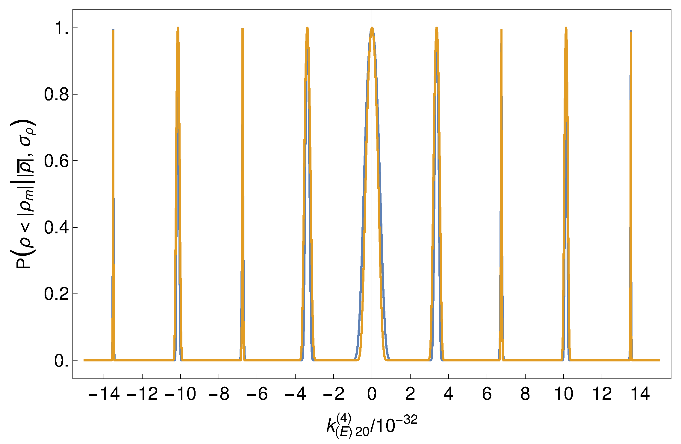
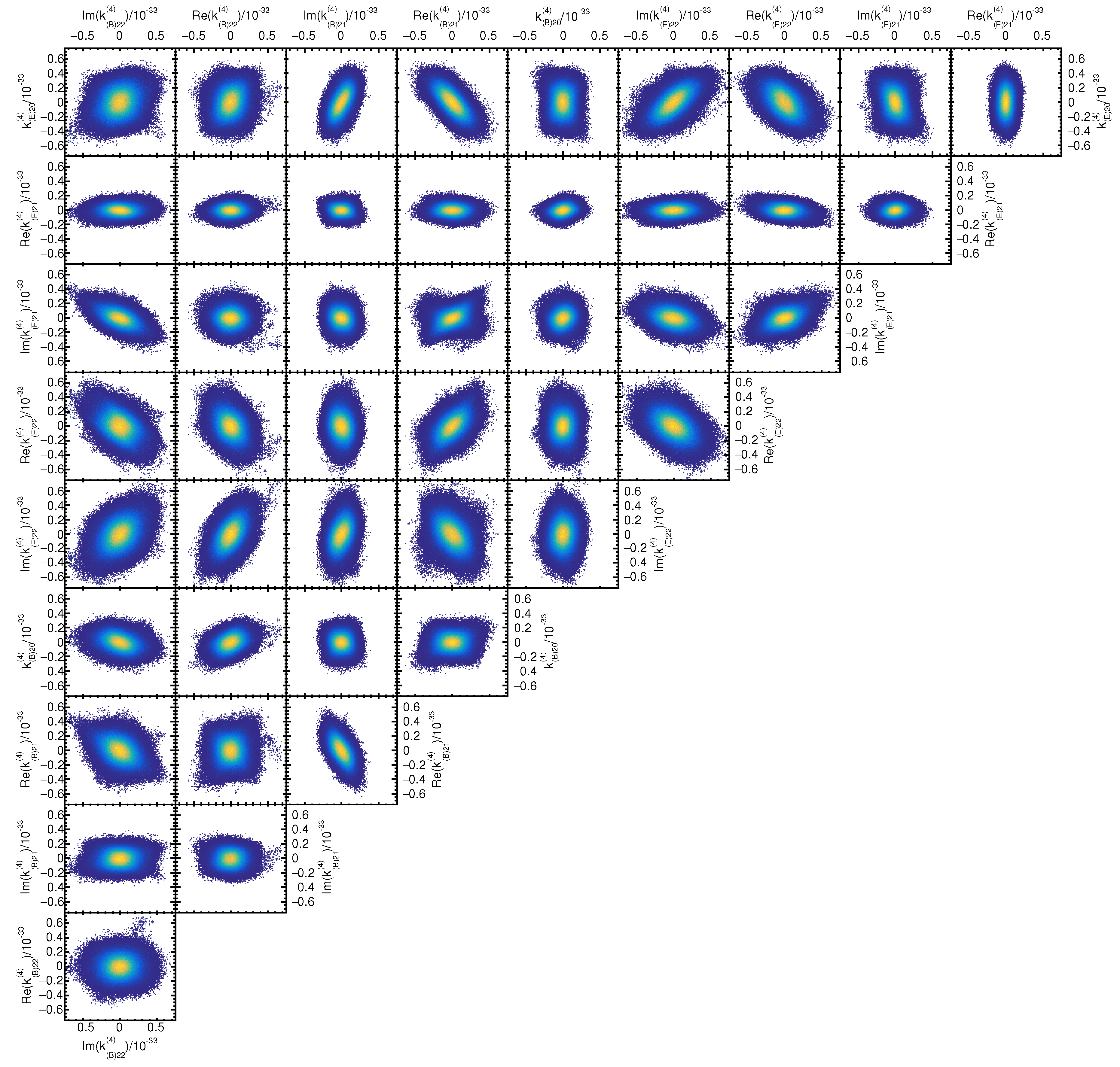
Appendix B. Coefficient Distributions and Correlations


References
- Michelson, A.A.; Morley, E.W. On the Relative Motion of the Earth and the Luminiferous Aether. Phil. Mag. 1887, 24, 449. [Google Scholar] [CrossRef]
- Kennedy, R.J.; Thorndike, E.M. Experimental Establishment of the Relativity of Time. Phys. Rev. 1932, 42, 400–418. [Google Scholar] [CrossRef]
- Ives, H.E.; Stilwell, G.R. An Experimental study of the rate of a moving atomic clock. J. Opt. Soc. Am. 1938, 28, 215. [Google Scholar] [CrossRef]
- Kostelecký, V.A.; Russell, N. Data Tables for Lorentz and CPT Violation. Rev. Mod. Phys. 2011, 83, 11–31, [updated at arXiv:hep-ph/0801.0287v11]. [Google Scholar] [CrossRef]
- Amelino-Camelia, G.; Ellis, J.; Mavromatos, N.E.; Nanopoulos, D.V.; Sarkar, S. Tests of quantum gravity from observations of γ-ray bursts. Nature 1998, 393, 763–765. [Google Scholar] [CrossRef]
- Garay, L.J. Spacetime Foam as a Quantum Termal Bath. Phys. Rev. Lett. 1998, 80, 2508–2511. [Google Scholar] [CrossRef]
- Gambini, R.; Pullin, J. Nonstandard optics from quantum space-time. Phys. Rev. D 1999, 59, 124021. [Google Scholar] [CrossRef]
- Mattingly, D. Modern Tests of Lorentz Invariance. Living Rev. Relativity 2005, 8, 5. Available online: http://www.livingreviews.org/lrr-2005-5 (accessed on 31 August 2018). [CrossRef] [PubMed]
- Jacobson, T.; Liberati, S.; Mattingly, D. Lorentz violation at high energy: Concepts, phenomena, and astrophysical constraints. Ann. Phys. 2006, 321, 150–196. [Google Scholar] [CrossRef]
- Liberati, S.; Maccione, L. Lorentz Violation: Motivation and New Constraints. Annu. Rev. Nucl. Part. Sci. 2009, 59, 245–267. [Google Scholar] [CrossRef]
- Kostelecký, V.A.; Mewes, M. Astrophysical Tests of Lorentz and CPT Violation with Photons. Astrophys. J. Lett. 2008, 689, L1–L4. [Google Scholar] [CrossRef]
- Kostelecký, V.A.; Mewes, M. Electrodynamics with Lorentz-violating operators of arbitrary dimension. Phys. Rev. D 2009, 80, 015020. [Google Scholar] [CrossRef]
- Abdo, A.A.; Ackermann, M.; Ajello, M.; Asano, K.; Atwood, W.B.; Axelsson, M.; Baldini, L.; Ballet, J.; Barbiellini, G.; Baring, M.G.; et al. A limit on the variation of the speed of light arising from quantum gravity effects. Nature 2009, 462, 331–334. [Google Scholar] [CrossRef] [PubMed]
- Vasileiou, V.; Jacholkowska, A.; Piron, F.; Bolmont, J.; Couturier, C.; Granot, J.; Stecker, F.W.; Cohen-Tanugi, J.; Longo, F. Constraints on Lorentz invariance violation from Fermi-Large Area Telescope observations of gamma-ray bursts. Phys. Rev. D 2013, 87, 122001. [Google Scholar] [CrossRef]
- Abramowski, A.; Aharonian, F.; Ait Benkhali, F.; Akhperjanian, A.G.; Angüner, E.O.; Backes, M.; Balenderan, S.; Balzer, A.; Barnacka, A.; Becherini, Y.; et al. The 2012 Flare of PG 1553+113 Seen with H.E.S.S. and Fermi-LAT. Astrophys. J. 2015, 802, 65. [Google Scholar] [CrossRef]
- Kislat, F.; Krawczynski, H. Search for anisotropic Lorentz invariance violation with γ-rays. Phys. Rev. D 2015, 92, 045016. [Google Scholar] [CrossRef]
- Wei, J.J.; Wu, X.F.; Zhang, B.B.; Shao, L.; Mészáros, P.; Kostelecký, V.A. Constraining Anisotropic Lorentz Violation via the Spectral-lag Transition of GRB 160625B. Astrophys. J. 2017, 842, 115. [Google Scholar] [CrossRef]
- Kaaret, P. X-ray clues to viability of loop quantum gravity. Nature 2004, 427, 287. [Google Scholar] [CrossRef] [PubMed]
- Kostelecký, V.A.; Mewes, M. Constraints on Relativity Violations from Gamma-Ray Bursts. Phys. Rev. Lett. 2013, 110, 201601. [Google Scholar] [CrossRef] [PubMed]
- Kislat, F.; Krawczynski, H. Planck-scale constraints on anisotropic Lorentz and CPT invariance violations from optical polarization measurements. Phys. Rev. D 2017, 95, 083013. [Google Scholar] [CrossRef]
- Komatsu, E.; Smith, K.M.; Dunkley, J.; Bennett, C.L.; Gold, B.; Hinshaw, G.; Jarosik, N.; Larson, D.; Nolta, M.R.; Page, L.; et al. Seven-year Wilkinson Microwave Anisotropy Probe (WMAP) Observations: Cosmological Interpretation. Astrophys. J. Suppl. Ser. 2011, 192, 18. [Google Scholar] [CrossRef]
- Brown, M.L.; Ade, P.; Bock, J.; Bowden, M.; Cahill, G.; Castro, P.G.; Church, S.; Culverhouse, T.; Friedman, R.B.; Ganga, K.; et al. Improved Measurements of the Temperature and Polarization of the Cosmic Microwave Background from QUaD. Astrophys. J. 2009, 705, 978–999. [Google Scholar] [CrossRef]
- Pagano, L.; de Bernardis, P.; de Troia, G.; Gubitosi, G.; Masi, S.; Melchiorri, A.; Natoli, P.; Piacentini, F.; Polenta, G. CMB polarization systematics, cosmological birefringence, and the gravitational waves background. Phys. Rev. D 2009, 80, 043522. [Google Scholar] [CrossRef]
- Kostelecký, V.A.; Melissinos, A.C.; Mewes, M. Searching for photon-sector Lorentz violation using gravitational-wave detectors. Phys. Lett. B 2016, 761, 1–7. [Google Scholar] [CrossRef]
- Contopoulos, G.; Jappel, A. Transactions of the International Astronomical Union, Volume XVB. In Proceedings of the Fifteenth General Assembly, Sydney 1973 and Extraordinary Assembly, Poland 1973; Springer Science & Business Media: Berlin, Germany, 1980. [Google Scholar]
- Smith, P.S.; Montiel, E.; Rightley, S.; Turner, J.; Schmidt, G.D.; Jannuzi, B.T. Coordinated Fermi/Optical Monitoring of Blazars and the Great 2009 September Gamma-ray Flare of 3C 454.3. Available online: http://arxiv.org/abs/0912.3621 (accessed on 6 September 2018).
- SVO Filter Profile Service. Available online: http://svo2.cab.inta-csic.es/svo/theory/fps3/index.php?&mode=browse&gname=NOT&gname2=ALFOSC&all=0 (accessed on 23 November 2015).
- O’Brien, K.; Marconi, G.; Dumas, C. Very Large Telescope Paranal Science Operations FORS User Manual; Technical Report VLT-MAN-ESO-13100-1543, Version 82.1; European Southern Observatory: Garching, Germany, 2008. [Google Scholar]
- Boffin, H.; Dumas, C.; Kaufer, A. Very Large Telescope Paranal Science Operations FORS2 User Manual; Technical Report VLT-MAN-ESO-13100-1543, Version 96.0; European Southern Observatory: Garching, Germany, 2015. [Google Scholar]
- Hau, G.K.T.; Patat, F. EFOSC2 User’s Manual; Technical Report LSO-MAN-ESO-36100-0004, Version 2.0; European Southern Observatory: Garching, Germany, 2003. [Google Scholar]
- Kawabata, K.S.; Nagae, O.; Chiyonobu, S.; Tanaka, H.; Nakaya, H.; Suzuki, M.; Kamata, Y.; Miyazaki, S.; Hiragi, K.; Miyamoto, H.; et al. Wide-field one-shot optical polarimeter: HOWPol. In Ground-Based and Airborne Instrumentation for Astronomy II; SPIE: Marseille, France, 2008; Volume 7014, p. 70144L. [Google Scholar]
- Marscher, A.P. Turbulent, Extreme Multi-zone Model for Simulating Flux and Polarization Variability in Blazars. Astrophys. J. 2014, 780, 87. [Google Scholar] [CrossRef]
- Zhang, H.; Li, H.; Guo, F.; Taylor, G. Polarization Signatures of Kink Instabilities in the Blazar Emission Region from Relativistic Magnetohydrodynamic Simulations. Astrophys. J. 2017, 835, 125. [Google Scholar] [CrossRef]
- Scarpa, R.; Falomo, R. Are high polarization quasars and BL Lacertae objects really different? A study of the optical spectral properties. Astron. Astrophys. 1997, 325, 109–123. [Google Scholar]
- Deng, W.; Zhang, B.; Li, H.; Stone, J.M. Magnetized Reverse Shock: Density-fluctuation-induced Field Distortion, Polarization Degree Reduction, and Application to GRBs. Astrophys. J. Lett. 2017, 845, L3. [Google Scholar] [CrossRef]
- Weisskopf, M.C.; Elsner, R.F.; Kaspi, V.M.; O’Dell, S.L.; Pavlov, G.G.; Ramsey, B.D. X-Ray Polarimetry and Its Potential Use for Understanding Neutron Stars. In Astrophysics and Space Science Library; Becker, W., Ed.; Springer: Berlin, Germany, 2009; Volume 357, p. 589. [Google Scholar]
- Krawczynski, H. Analysis of the data from Compton X-ray polarimeters which measure the azimuthal and polar scattering angles. Astropart. Phys. 2011, 34, 784–788. [Google Scholar] [CrossRef]
- Sluse, D.; Hutsemékers, D.; Lamy, H.; Cabanac, R.; Quintana, H. New optical polarization measurements of quasi-stellar objects. The data. Astron. Astrophys. 2005, 433, 757–764. [Google Scholar] [CrossRef]
- Sluse, D.; Hutsemékers, D.; Lamy, H.; Cabanac, R.; Quintana, H. Optical Polarization of 203 QSOs (Sluse+, 2005). Available online: http://vizier.u-strasbg.fr/viz-bin/VizieR?-source=J/A+A/433/757 (accessed on 6 September 2018).
- Covino, S.; Götz, D. Polarization of prompt and afterglow emission of Gamma-Ray Bursts. Astron. Astrophys. Trans. 2016, 29, 205–244. [Google Scholar]
- Wijers, R.A.M.J.; Vreeswijk, P.M.; Galama, T.J.; Rol, E.; van Paradijs, J.; Kouveliotou, C.; Giblin, T.; Masetti, N.; Palazzi, E.; Pian, E.; et al. Detection of Polarization in the Afterglow of GRB 990510 with the ESO Very Large Telescope. Astrophys. J. 1999, 523, L33–L36. [Google Scholar] [CrossRef]
- Covino, S.; Lazzati, D.; Ghisellini, G.; Saracco, P.; Campana, S.; Chincarini, G.; di Serego, S.; Cimatti, A.; Vanzi, L.; Pasquini, L.; et al. GRB 990510: Linearly polarized radiation from a fireball. Astron. Astrophys. 1999, 348, L1–L4. [Google Scholar]
- Covino, S.; Lazzati, D.; Ghisellini, G.; Saracco, P.; Campana, S.; Chincarini, G.; di Serego Alighieri, S.; Cimatti, A.; Vanzi, L.; Pasquini, L.; et al. GRB 990510. IAU Circ. 1999, 7172, 3. [Google Scholar]
- Rol, E.; Wijers, R.A.M.J.; Vreeswijk, P.M.; Kaper, L.; Galama, T.J.; van Paradijs, J.; Kouveliotou, C.; Masetti, N.; Pian, E.; Palazzi, E.; et al. GRB 990712: First Indication of Polarization Variability in a Gamma-Ray Burst Afterglow. Astrophys. J. 2000, 544, 707–711. [Google Scholar] [CrossRef]
- Rol, E.; Wijers, R.A.M.J.; Fynbo, J.P.U.; Hjorth, J.; Gorosabel, J.; Egholm, M.P.; Castro Cerón, J.M.; Castro-Tirado, A.J.; Kaper, L.; Masetti, N.; et al. Variable polarization in the optical afterglow of GRB 021004. Astron. Astrophys. 2003, 405, L23–L27. [Google Scholar] [CrossRef]
- Greiner, J.; Klose, S.; Reinsch, K.; Martin Schmid, H.; Sari, R.; Hartmann, D.H.; Kouveliotou, C.; Rau, A.; Palazzi, E.; Straubmeier, C.; et al. Evolution of the polarization of the optical afterglow of the γ-ray burst GRB030329. Nature 2003, 426, 157–159. [Google Scholar] [CrossRef] [PubMed]
- Gorosabel, J.; Rol, E.; Covino, S.; Castro-Tirado, A.J.; Castro Cerón, J.M.; Lazzati, D.; Hjorth, J.; Malesani, D.; Della Valle, M.; di Serego Alighieri, S.; et al. GRB 020813: Polarization in the case of a smooth optical decay. Astron. Astrophys. 2004, 422, 113–119. [Google Scholar] [CrossRef]
- Barth, A.J.; Sari, R.; Cohen, M.H.; Goodrich, R.W.; Price, P.A.; Fox, D.W.; Bloom, J.S.; Soderberg, A.M.; Kulkarni, S.R. Optical Spectropolarimetry of the GRB 020813 Afterglow. Astrophys. J. 2003, 584, L47–L51. [Google Scholar] [CrossRef]
- Wiersema, K.; Curran, P.A.; Krühler, T.; Melandri, A.; Rol, E.; Starling, R.L.C.; Tanvir, N.R.; van der Horst, A.J.; Covino, S.; Fynbo, J.P.U.; et al. Detailed optical and near-infrared polarimetry, spectroscopy and broad- band photometry of the afterglow of GRB 091018: Polarization evolution. Mon. Not. Royal Astron. Soc. 2012, 426, 2–22. [Google Scholar] [CrossRef]
- Uehara, T.; Toma, K.; Kawabata, K.S.; Chiyonobu, S.; Fukazawa, Y.; Ikejiri, Y.; Inoue, T.; Itoh, R.; Komatsu, T.; Miyamoto, H.; et al. GRB 091208B: First Detection of the Optical Polarization in Early Forward Shock Emission of a Gamma-Ray Burst Afterglow. Astrophys. J. 2012, 752, L6. [Google Scholar] [CrossRef]
- Wiersema, K.; Covino, S.; Toma, K.; van der Horst, A.J.; Varela, K.; Min, M.; Greiner, J.; Starling, R.L.C.; Tanvir, N.R.; Wijers, R.A.M.J.; et al. Circular polarization in the optical afterglow of GRB 121024A. Nature 2014, 509, 201–204. [Google Scholar] [CrossRef] [PubMed]
- Steele, I.A.; Mundell, C.G.; Smith, R.J.; Kobayashi, S.; Guidorzi, C. Ten per cent polarized optical emission from GRB090102. Nature 2009, 462, 767–769. [Google Scholar] [CrossRef] [PubMed]
- Hastings, W.K. Monte Carlo Sampling Methods using Markov Chains and their Applications. Biometrika 1970, 57, 97–109. [Google Scholar] [CrossRef]
- Bolokhov, P.A.; Groot Nibbelink, S.; Pospelov, M. Lorentz violating supersymmetric quantum electrodynamics. Phys. Rev. D 2005, 72, 015013. [Google Scholar] [CrossRef]
- Tanabashi, M.; Hagiwara, K.; Hikasa, K.; Nakamura, K.; Sumino, Y.; Takahashi, F.; Tanaka, J.; Agashe, K.; Aielli, G.; Amsler, C.; et al. Review of Particle Physics. Phys. Rev. D 2018, 98, 030001. [Google Scholar] [CrossRef]
- Weisskopf, M.C.; Ramsey, B.; O’Dell, S.L.; Tennant, A.; Elsner, R.; Soffita, P.; Bellazzini, R.; Costa, E.; Kolodziejczak, J.; Kaspi, V.; et al. The Imaging X-ray Polarimetry Explorer (IXPE). Results Phys. 2016, 6, 1179–1180. [Google Scholar] [CrossRef]
- Moiseev, A. All-Sky Medium Energy Gamma-ray Observatory (AMEGO). Proc. Sci. 2018, ICRC2017, 798. [Google Scholar]
- Yang, C.Y.; Lowell, A.; Zoglauer, A.; Tomsick, J.; Chiu, J.L.; Kierans, C.; Sleator, C.; Boggs, S.; Chang, H.K.; Jean, P.; et al. The polarimetric performance of the Compton Spectrometer and Imager (COSI). In Society of Photo-Optical Instrumentation Engineers (SPIE) Conference Series; SPIE: Austin, TX, USA, 2018; Volume 10699, p. 106992K. [Google Scholar]
- Wenger, M.; Ochsenbein, F.; Egret, D.; Dubois, P.; Bonnarel, F.; Borde, S.; Genova, F.; Jasniewicz, G.; Laloë, S.; Lesteven, S.; et al. The SIMBAD astronomical database. The CDS reference database for astronomical objects. Astron. Astrophys. Suppl. Ser. 2000, 143, 9–22. [Google Scholar] [CrossRef]
- Barkhouse, W.A.; Hall, P.B. Quasars in the 2MASS Second Incremental Data Release. Astron. J. 2001, 121, 2843–2850. [Google Scholar] [CrossRef]
- Shaw, M.S.; Romani, R.W.; Cotter, G.; Healey, S.E.; Michelson, P.F.; Readhead, A.C.S.; Richards, J.L.; Max-Moerbeck, W.; King, O.G.; Potter, W.J. Spectroscopy of Broad-line Blazars from 1LAC. Astrophys. J. 2012, 748, 49. [Google Scholar] [CrossRef]
- Mao, L.S. 2MASS observation of BL Lac objects II. New Astron. 2011, 16, 503–529. [Google Scholar] [CrossRef]
- Abazajian, K.N.; Adelman-McCarthy, J.K.; Agüeros, M.A.; Allam, S.S.; Allende Prieto, C.; An, D.; Anderson, K.S.J.; Anderson, S.F.; Annis, J.; Bahcall, N.A.; et al. The Seventh Data Release of the Sloan Digital Sky Survey. Astrophys. J. Suppl. Ser. 2009, 182, 543–558. [Google Scholar] [CrossRef]
- Halpern, J.P.; Eracleous, M.; Mattox, J.R. Redshifts of Candidate Gamma-Ray Blazars. Astron. J. 2003, 125, 572–579. [Google Scholar] [CrossRef]
- Enya, K.; Yoshii, Y.; Kobayashi, Y.; Minezaki, T.; Suganuma, M.; Tomita, H.; Peterson, B.A. JHK’ Imaging Photometry of Seyfert 1 Active Galactic Nuclei and Quasars. I. Multiaperture Photometry. Astrophys. J. Suppl. Ser. 2002, 141, 23–29. [Google Scholar] [CrossRef]
- Donato, D.; Ghisellini, G.; Tagliaferri, G.; Fossati, G. Hard X-ray properties of blazars. Astron. Astrophys. 2001, 375, 739–751. [Google Scholar] [CrossRef]
- Jones, D.H.; Read, M.A.; Saunders, W.; Colless, M.; Jarrett, T.; Parker, Q.A.; Fairall, A.P.; Mauch, T.; Sadler, E.M.; Watson, F.G.; et al. The 6dF Galaxy Survey: Final redshift release (DR3) and southern large- scale structures. Mon. Not. Royal Astron. Soc. 2009, 399, 683–698. [Google Scholar] [CrossRef]
- Kovalev, Y.Y.; Nizhelsky, N.A.; Kovalev, Y.A.; Berlin, A.B.; Zhekanis, G.V.; Mingaliev, M.G.; Bogdantsov, A.V. Survey of instantaneous 1–22 GHz spectra of 550 compact extragalactic objects with declinations from -30deg to +43deg. Astron. Astrophy. Suppl. 1999, 139, 545–554. [Google Scholar] [CrossRef]


| Instrument | Filter | [10−10 GeV] |
|---|---|---|
| FORS1 | R-band | 3.840 |
| FORS1 | V-band | 3.926 |
| FORS2 | 4.548 | |
| ALFOSC | R-band | 3.135 |
| EFOSCV | V-band | 3.763 |
| HOWPol | R-band | 3.611 |
| < 2.4 × 10⁻³⁴ | |
| < 1.0 × 10⁻³⁴ | |
| < 1.6 × 10⁻³⁴ | |
| < 2.4 × 10⁻³⁴ | |
| < 2.6 × 10⁻³⁴ | |
| < 1.5 × 10⁻³⁴ | |
| < 2.2 × 10⁻³⁴ | |
| < 1.4 × 10⁻³⁴ | |
| < 1.9 × 10⁻³⁴ | |
| < 2.5 × 10⁻³⁴ |
© 2018 by the author. Licensee MDPI, Basel, Switzerland. This article is an open access article distributed under the terms and conditions of the Creative Commons Attribution (CC BY) license (http://creativecommons.org/licenses/by/4.0/).
Share and Cite
Kislat, F. Constraints on Lorentz Invariance Violation from Optical Polarimetry of Astrophysical Objects. Symmetry 2018, 10, 596. https://doi.org/10.3390/sym10110596
Kislat F. Constraints on Lorentz Invariance Violation from Optical Polarimetry of Astrophysical Objects. Symmetry. 2018; 10(11):596. https://doi.org/10.3390/sym10110596
Chicago/Turabian StyleKislat, Fabian. 2018. "Constraints on Lorentz Invariance Violation from Optical Polarimetry of Astrophysical Objects" Symmetry 10, no. 11: 596. https://doi.org/10.3390/sym10110596
APA StyleKislat, F. (2018). Constraints on Lorentz Invariance Violation from Optical Polarimetry of Astrophysical Objects. Symmetry, 10(11), 596. https://doi.org/10.3390/sym10110596