A Comparison of Regularization Techniques in Deep Neural Networks

Abstract

Artificial neural networks (ANN) have attracted significant attention from researchers because many complex problems can be solved by training them. If enough data are provided during the training process, ANNs are capable of achieving good performance results. However, if training data are not enough, the predefined neural network model suffers from overfitting and underfitting problems. To solve these problems, several regularization techniques have been devised and widely applied to applications and data analysis. However, it is difficult for developers to choose the most suitable scheme for a developing application because there is no information regarding the performance of each scheme. This paper describes comparative research on regularization techniques by evaluating the training and validation errors in a deep neural network model, using a weather dataset. For comparisons, each algorithm was implemented using a recent neural network library of TensorFlow. The experiment results showed that an autoencoder had the worst performance among schemes. When the prediction accuracy was compared, data augmentation and the batch normalization scheme showed better performance than the others.

1. Introduction

Accurate weather forecasting is an important issue that plays a significant role in the development of several industrial sectors, such as agriculture and transportation. Many companies are using weather prediction techniques to analyze consumer demands. In addition, exact forecasting is essential for people to organize and plan their days. However, it is very difficult to predict the weather precisely because the atmosphere changes dynamically. For a long time, physical simulations were the most widely used scheme. With this method, the current atmospheric condition is sampled, and future conditions are predicted by comparing thermodynamic characteristics. In recent years, artificial neural networks (ANNs) have been widely used for weather prediction because they perform better through the use of machine learning. The human brain is composed of 100 billion interconnected neurons. These neurons are core cells that are responsible for information transmission among neurons using electrochemical signals.

ANNs were modeled by using a mechanism inspired by the human brain’s information processing. This scheme was first introduced to researchers in 1943 by Warren and Walter [1]. This scheme is currently being used in almost every scientific area to solve complex problems. Williams [2] presented the efficiency of machine learning algorithms, and proved that they could be applied to many applications. Nicholas [3] proposed an enhanced scheme to train neural network algorithms. In the scheme, a statistical computation scheme was used to reduce the training errors. Zhang [4] proposed a new recurrent neural network (RNN) scheme based on synchronization of delays and impulses, which reduced prediction errors. Isomura [5] applied neural networks to knowledge inference applications, useful information was collected, and an inference rule was extracted using deep neural networks (DNNs). Elusai [6] used ANNs to model behavior to prevent bronze corrosion. In the scheme, corrosion types were classified into different features, and future corrosion behaviors were predicted. Jian [7] enhanced an existing principal component analysis (PCA) neural network that was based on new discrete-time algorithms. The experiment results showed that validation errors were significantly decreased. Yin [8] applied a DNN to classify server states for enhancing the quality of service in cloud environments. The experiments showed that the scheme could be used to find used or broken servers.

During the training process, the input data type and amount directly influence the performance of the ANN model [9]. If the training data are deficient, overfitting or underfitting occurs [10]. Overfitting refers to the phenomenon where the validation error increases while the training error decreases [11]. This occurs because the model learns the expected output for every input data instead of learning the real data distribution [12,13]. In contrast, underfitting problems occur when a model cannot learn enough because of insufficient training data [14,15]. Many solutions have been proposed to prevent these problems. The most widely used method is regularization, where a small variation is applied to the original data to efficiently train a model [16]. One of the advantages of this method is that it achieves a better performance for unseen data. For weather prediction, it is used to predict rainfall, temperature, and humidity [17].

In this study, we summarize prior research on weather prediction using ANNs. Several studies have been completed on accurately predicting the weather. There studies included a method based on an ANN model to predict the air temperature at hourly intervals for up to 12 h [18,19]. The prediction error was minimized, and the method achieved good performance for short-term forecasting. Other research [20,21] developed a new model to predict the hourly temperature for up to 24 hour. The model used a separate winter, spring, summer, and fall season. Experiments were conducted to compare the performances of well-known ANN models, including the Elman recurrent neural network (ERNN), the radial basis function network (RBFN), the multilayer perceptron network (MLP), and the Hopfield model (HFM). The MLP model with a single hidden layer and the RBFN model with two hidden layers outperformed the other models. In the MLP experiment, the log-sigmoid function was used as the activation function, and the Gaussian activation function was used for the hidden layers in the RBFN. The temperatures for both models were measured and drawn with pure lines. Although the accuracy of both models was identical, the RBFN had better processing times, because it took too long for the MLP to learn data. Some research compared several ANN models by applying various transfer functions, hidden layers, and neurons to predict the maximum temperature for the year. The model included five hidden layers, and each hidden layer contained 10 or 16 neurons. The tan-sigmoid activation function for hidden layers showed the bests results when using the logistic sigmoid function [22]. Xiaodong [23] presented a data augmentation scheme to improve performance when applied to audio data. In the scheme, extra sampling data were added to the original input audio data and used for training and validation. Huaguang [24] analyzed the stability of RNNs. An RNN was the most widely used scheme in analyzing and predicting time series data. Songchuan [25] proposed a new training algorithm, called fireworks, to predict the mean temperature. The algorithm showed fast convergence and reduced training cycles. Takashi [26] proposed a new RNN algorithm that was based on asynchronous negotiation and reproduction. This algorithm improved the prediction efficiency when it was applied to time series data. Hayati [27] used an ANN model that contained a single hidden layer and six neurons, which showed good performance results. Many of the latest advances can be found in image processing and object detection. Cao [28] invented a fast DNN algorithm based on additional knowledge during training. This was applied to object detection from streaming video, and the results showed that it could reach good performance. Wang [29] applied a convolutional neural network (CNN) to detecting a salient object from input images. A salient object refers to the most important object, which expresses the most outstanding characteristic from an image. To do this, they used additional metadata together with a CNN. Yue [30] applied neural networks to detecting a collision between cars. The video streaming captured from the traffic system was very complex and dynamic. This made collision detection more difficult. To solve this problem, they presented an enhanced DNN algorithm that was based on feature enhancement. Huang [31] used a neural network to improve the detection accuracy of traffic monitoring systems. One of the problems in moving object detection is that the accuracy becomes lower when there are too many moving objects in a video stream. To solve this problem, they used a DNN to detect a moving object accurately. Akcay [32] used a deep convolutional neural network (DCNN) to classify and detect an object from X-ray images scanned in an airport. By using this, they could save time and expense spent in investigating and detecting a dangerous object. Sevo [33] used a CNN to detect an object from images captured in the air. It is very difficult to detect an object from the air because all scenes in the air are expressed as three-dimensional (3D) images. By using a CNN, he could decrease the complexity of air object detection. One of the most widely known areas where neural networks are applied can be said to be image processing. Woźniak [34] presented an enhanced object detection method, where convolutional neural networks were combined with the analysis of clustered numbers. To determine the points of clusters, they used fuzzy logic. Vieira [35] presented methods and applications of deep learning that were applied to neuroimaging. Neuroimaging is used to make an image structure of a human brain to cure mental disease. In their paper, they insisted that deep learning could be an efficient method in improving brain image quality by training the neural network. Polap [36] described a practice in which an ANN was applied to detect potential diseases from body skin. In the method, skin data were collected by using motion sensors and a camera, and an ANN model was trained using the data. Then, using the model, they determined whether the skin had disease or not. Heaton [37] described an application of deep-learning stochastic models in financial areas. In these areas, they used deep learning to predict and classify financial data. Most doctors in hospitals used X-rays to classify carcinomas in chest organs. However, it causes wrong diagnoses because it is difficult for radiologists to exactly interpret the X-ray results. To solve this problem, Wozniak [38] applied neural networks to improving the accuracies of carcinoma classification. The experimental results showed that they reached a 92% classification accuracy. Litjens [39] described recent advancements of deep learning applications in analyzing images in the medical industry. In the paper, they presented more than 300 pieces of research achieved in this field. To give a concise review, they divided application areas for studies into 10 medical areas. Wozniak [40] presented a new method based on neural networks to detect defects of fruit peels, which was very different from a classical scheme. They invented an enhanced ANN algorithm called an adaptive artificial neural network (AANN). By using this method, they could improve calculation accuracy because it adapted to input data and their characteristics. Wang [41] presented an overview of machine learning applications for manufacturing. Through the help of widespread sensors and the Internet of Things (IoT), huge amounts of data could be collected in manufacturing systems. Deep learning could be used to improve system performance and product quality by analyzing collected big data.

As described earlier, active research is being conducted on neural networks and overfitting solutions. However, there is no research that compares regularization schemes. Therefore, it is difficult for developers to choose the most suitable scheme for developing an application, because there is no information about the performance of each scheme. To solve this problem, this study presents comparative research on regularization techniques by evaluating the training and validation errors in a DNN model using weather datasets. Especially, the appropriate choice of the regularization scheme is a very important process to manage huge augmented objects in intelligent mobile augmented reality (IMAR) system.

The remainder of this paper is organized as follows. Section 2 describes the research methodology and experiment setup. In Section 3, experiment results are described and analyzed. Section 4 presents a discussion of the results. Finally, Section 5 concludes this work.

2. Data and Methods

2.1. Methodology

The methodology of the comparative research is represented in Figure 1. The entire methodology consisted of 9 steps. To compare the performance, several powerful regularization methods, including an autoencoder, data augmentation, batch normalization, and L1 regularization, were implemented and studied. First, we built a DNN model without using any regularization methods. We then trained and validated the model, and then calculated the errors. Next, we measured the errors of the same model without changing the settings, after applying regularization schemes. Each regularization scheme was analyzed by comparing the experiment results. Each step is described in more detail in the following section.

First, the datasets that were used to train and validate the neural network model were collected. In our experiment, the Korean weather dataset was collected from the government website. It included 35 features, including average temperature, maximum temperature, minimum temperature, average wind speed, average humidity, cloudiness, and daylight hours, for the previous five days. The average temperature was a target feature to predict for the next day. We let x⁽ⁱ⁾ be a 35-dimensional feature vector for the ith set of five consecutive days, and let y⁽ⁱ⁾ be the one-dimensional vector that contained this feature for the ith single day. The prediction of y⁽ⁱ⁾ with a given x⁽ⁱ⁾ can be expressed using Equation (1):

Z(y⁽ⁱ⁾) = σ(θ(x⁽ⁱ⁾)).

(1)

In Equation (1), θ refers to a subset of the 35-dimensional vector, and σ is an activation function. The cost function seeks to minimize

$$Cost(\theta )=\frac{1}{2}{\sum }_{i=1}^m{(Z_{\theta }(x^{(i)})-y^{(i)})}^2.$$

(2)

In Equation (2), m is the number of training examples. For supervised machine learning, the data are typically divided into two types, training and testing data. However, to obtain a better tuning model, validation data were used in addition to the original data. These validation data are referred to as the development dataset, or dev dataset. The goal of this dataset was to fine-tune the hyper parameters (architecture) of the ANN model. The model frequently used this data. However, it did not learn from this dataset. This set had to be used to obtain the optimal number of hidden units. The dataset was divided using the Sci-Kit Learn library as follows. First, the data was split into training and temporary data. Approximately 80% of the entire dataset was used as training data, and 20% was used as temporary data. The temporary dataset was split into two equal parts, test and validation. Entire data usage for both training and verification would increase the inaccuracy of prediction and would increase the training errors. It would be better to use the divided dataset. We think that cross-samplings can be good ways to decrease the errors. However, we did not use these methods because we had to change the input algorithms in order to apply the cross-samplings. In future work, we can apply the algorithms.

Next, we defined and chose an accurate architecture for neural network analysis. This process usually requires significant experience because many factors must be efficiently decided. One factor is how many layers should be set in the model. The basic model included one input layer, two hidden layers, and one output layer, as illustrated in Figure 2. The input layer contained 35 neurons, the hidden layers contained 50 neurons each, and the output layer had 1 neuron. The topology of our model was the 35-50-50-1 topology.

After defining the model, we needed to make the parameter settings, which are listed in

Table 1. Parameter settings applied to a temperature prediction neural network model.

Parameters for Each Model	Typical DNN	Autoencoder	Data Augmentation	L1 Regularization	Batch Normalization
Number of input neurons	35	35	35	35	35
Number of hidden layers	2	2	2	2	2
Number of neurons in hidden layers	50	50	50	50	50
Number of output neurons	1	1	1	1	1
Learning rate	0.0001	0.0001	0.0001	0.0001	0.0001
Activation function	ReLU	ReLU	ReLU	ReLU	ReLU
Optimizer	Proximal Adagrad	Proximal Adagrad	Proximal Adagrad	Proximal Adagrad	Proximal Adagrad

. The columns included the basic DNN model and regularization schemes, and the rows included the parameters for each model. The first parameter was the number of input neurons. This number was set to 35 for most models, as previously described. The next parameter to set was the number of hidden layers, which were 2. In reality, the value could be increased or decreased according to the central processing unit (CPU) capability. If the CPU capability was high, the number could be decreased because it took less time. When tested in our experiment, 2 was the most appropriate value because the processing time increased exponentially if the value was greater than 3. The third was the number of neurons in the hidden layers. If the number was higher, then the results were better. However, there was a trade-off between the number and processing time. In our experiment, the value was set to be 50. The number of output neurons was set to 1 because the target feature had only one. The learning rate was set to 0.0001. Although processing took a long time because it was slightly low, the results were more reliable. The proximal Adagrad optimizer algorithm was used to optimize our model. The batch size was 100 and the maximum number of epochs was 100,000. The rectified linear unit (ReLU) was used for the activation function.

In the third step, a defined neural network model was trained using the original data where regularization methods were not applied. During training, the root mean square errors (RMSEs) were captured and the data were saved into a separate file. The RMSE value could be obtained using the following equation:

$$\mathrm{RMSE}({\mathrm{NN}}_{\mathrm{Model}})=\sqrt{\frac{1}{M}{\sum }_{i=1}^m{\left(\frac{Answer(X_i)-Predict(X_i)}{Answer(X_i)}\right)}^2}.$$

(3)

In Equation (3), Answer (X_i) is the real answer data at time i, and Predict (X_i) is the value predicted by the trained neural network model. In the fourth step, the defined neural network model was validated and the validation errors were captured using Equation (1). In the third and fourth steps, overfitting and underfitting were checked.

In the fifth step, regularization methods were applied to the original weather data. The applied methods will be described in more detail in Section 2.2. In steps 5 and 6, a defined model was trained and validated using the datasets. In step 7, the future temperature is predicted using the trained neural network model where regularization methods were applied. Finally, each scheme is compared by analyzing the train, validation, and prediction errors.

2.2. Applied Regularization Methods in the Experiment

This section describes the regularization methods for the experiment. A widely used scheme for regularization is the autoencoder scheme, which refers to an enhanced neural network with the same number of neurons in the input and output layers. This scheme uses unsupervised learning, because labels are not required when training the model. The scheme compresses the data received from the input neurons into short code, and then decompresses this code into output neurons that are very close to the input data. One of the goals of this scheme is to remove the noise from the input data. The architecture is similar to MLP structure, and it has at least one input, hidden, and output layer. This type of neural network consists of two parts, an encoder and a decoder. An encoder is a network component that compresses the input. A decoder is used to reconstruct the encoded input. In a simple autoencoder with a single layer, the encoder takes the x ϵ X input and compresses it to z ϵ Z. The equation for calculating the compressed data z is as follows [42]:

z = σ(W × x + b).

(4)

In Equation (4), z is known as the latent space representation. It is sometimes identified as a code or latent variable. Here, σ is the activation function, such as the ReLU, sigmoid, or Leaky ReLU function. W is the weight of the nodes, and b is the bias vector. In the reconstruction process, the same operation is repeated, as shown in Equation (5) [43]:

x′ = σ′(W′ × z + b′).

(5)

In the decoding process, the compressed data z is mapped to x′, where x′ represents the transformed input data with the same dimension as the input x value, and σ′ is an activation function used to decompress the data. W′ is the weight of the transformed nodes, and b′ is a bias in the decoder. To obtain satisfactory performance using the autoencoder scheme, the decoding loss should be minimized. Sum squared errors (SSEs) or an RMSE function were used to measure the loss as in Equation (6):

F(x, x′) = ||x − x′||2.

(6)

From Equations (3) and (4), we derived Equation (7):

f(x, x′) = ||x − σ′(W′z + b′)||2.

(7)

By replacing z with Equation (7), the final equation of the loss function was as follows [30]:

f(x, x′) = ||x − σ′(W′(σ(Wx + b)) + b′)||2.

(8)

There are many types of autoencoder schemes.

In our research, the stacked autoencoder was used to diminish the noise from the input data and simplify the tuning hyperparameters in a scheme. The architecture of the scheme is illustrated in Figure 3. It contained one input layer, three hidden layers, and one output layer.

Data augmentation is one of the most popular regularization techniques. The main idea of the scheme is to expand the training dataset by applying transformations to decrease overfitting. This technique is commonly used in image processing, since image operations like rotating, shifting, scaling, mirroring, or randomly cropping can be easily implemented when using the scheme [44]. For data augmentation, it is important to effectively control noise. There are some types of noise that are available for the scheme. Among them, the Gaussian noise control scheme is the most widely used. The scheme could be expressed using Equation (9) [45]:

L_min = Ep [(y − f(x + μ))2].

(9)

In Equation (9), μ is the noise vector. This technique is effectively used for RNNs, whereas it is seldom used in feed forward neural networks [46]. In this study, two augmentation techniques were implemented. The first type of data augmentation was to sum up partial datasets. Let $L_j^{(i)}$ represent input feature data for weather prediction, where j ∈ {1, 2, … n} is the number of features and i ∈ {1, 2, … m} is the number of identical categorical features (in our case, i is the number of days). The final input using the augmented data for the jth categorical data could be expressed as

$$\mathrm{input}\_{\mathrm{data}}_j=\frac{1}{m}{\sum }_{i=1}^m{L}_j^{(i)},$$

(10)

where L_j is the average humidity or average temperature. The number of input features is seven (j = 7), and the number of identical features is five (i = 5). The second augmentation summed the identical categorical features, as shown in Equation (11):

$$\mathrm{input}\_{\mathrm{data}}_j={\sum }_{i=1}^m{L}_j^{(i)}.$$

(11)

Similar to the first data augmentation technique, the number of input neurons became 7. The number of operations in the model decreased as the number of input data decreased, thereby preventing overfitting.

The third scheme for regularization was batch normalization, which was proposed by Sergey and Christian in 2015. After implementing batch normalization on a DNN, regularization techniques like dropout [47] or L2 regularization were not required to tune the model. Instead, this method focused on an internal covariate shift [48]. In addition, by implementing this method, they reduced the training time of the model.

The fourth scheme applied in the experiment was an L1 regularization. L1 regularization is known as the least absolute shrinkage and selection operator (LASSO), and was introduced by Robert [49]. The main idea behind the scheme is to regularize the loss function by completely removing the irrelevant features from the model [36]. The equation of the scheme could be expressed as

$$f(w,b)=\frac{1}{m}{\sum }_{i=1}^{m}L(\overline{y_i},y_i)-\lambda {\sum }_{j=1}^m\left|w_j\right|.$$

(12)

In Equation (12), $L(\overline{y_i},y_i)$ is a loss function, m is the number of observations, $\overline{y_i}$ is the predicted value (whereas $y_i$ is the actual value), and λ is a non-negative regularization parameter. The main objective was to minimize the f(w,b) function by penalizing weights in proportion to the sum of their absolute values. As λ increases, w decreases. As λ″ decreases, the variance increases.

2.3. Experiment Setup

The hardware specification for the experiment was as follows. The desktop used was a Gigabyte Z97X-UD3H personal computer running Windows 10 with an Intel Core i7-4790 K CPU and 8 GB of RAM. The simulations were implemented using Python programming language and the TensorFlow library. This library is very popular among machine learning application developers. A neural network application can run on several CPUs and graphics processing units (GPUs) in parallel. Supporting parallelism is one of the key features of the library. In addition, the library can be available for multiple programming languages, such as Python, C++, and Java. There are many higher-level application programming interfaces (APIs) that work with TensorFlow. For instance, Keras API, TFLearn, and Sonnet are provided to easily train the model. In our study, we implemented TensorFlow’s new higher-level constructs estimator. There were many advantages to the estimator:

• Without changing the model, our model could be run on local or distributed servers. In addition, without the need to record our model, our estimator-based model could run CPUs, GPUs, or tensor processing unit (TPU)s.
• It was much easier to develop a model with an estimator rather than low-level TensorFlow APIs.
• It could make a graph for us.

The estimator API provided an ordinary interface to train, evaluate, and predict functions. For building our model, we used DNNRegressor class in the tf.estimator package. There were many parameters in this class, but we will focus on the major ones as follows.

• Activation_fn: The activation function was for each layer of the neural network. By default, ReLU was fixed for the layers.
• Optimizer: In this feature of the class, we defined the optimizer type, which optimized the neural network model’s weights throughout the training process.
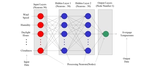
• Hidden_units: This contained the number of hidden units (neurons) per layer. For example, in [50], it means the first layer has 70 neurons and the second one has 50.
• Feature_columns: This argument contained the feature columns and data type used by the model.
• Model_dir: This was the directory for saving model parameters and graphs. In addition, it could be used to load checkpoints from the directory into the estimator to continue training a previously saved model.
• Dropout: We needed this feature for implementing a dropout regularization technique in our model.

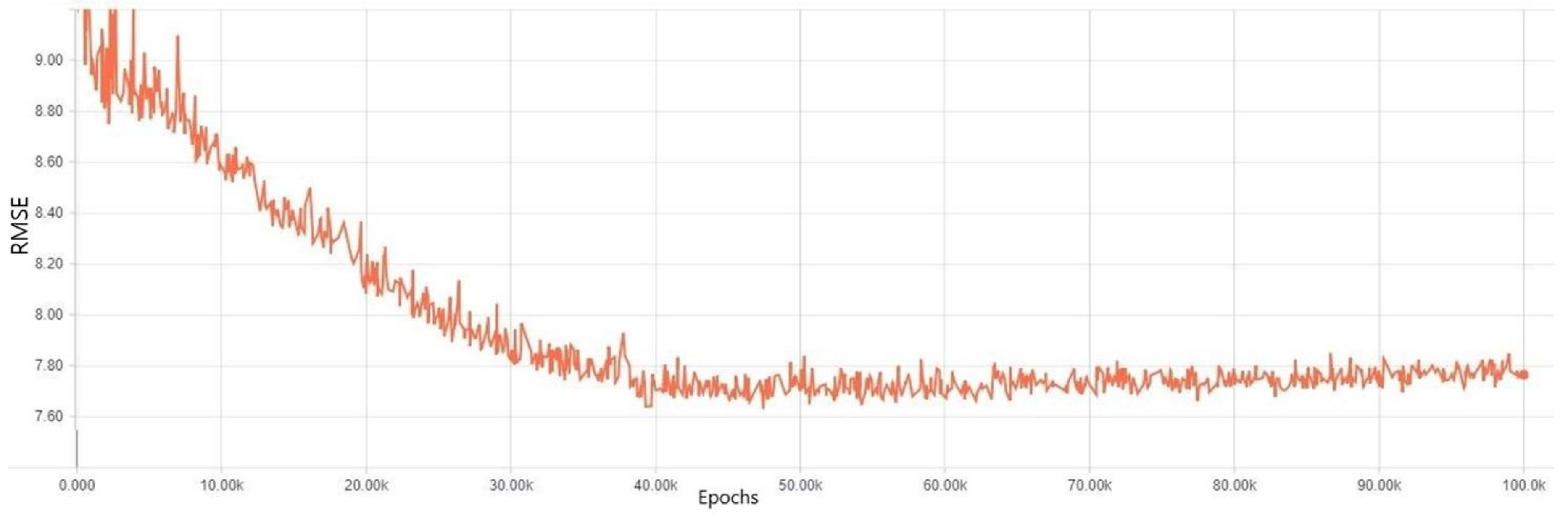
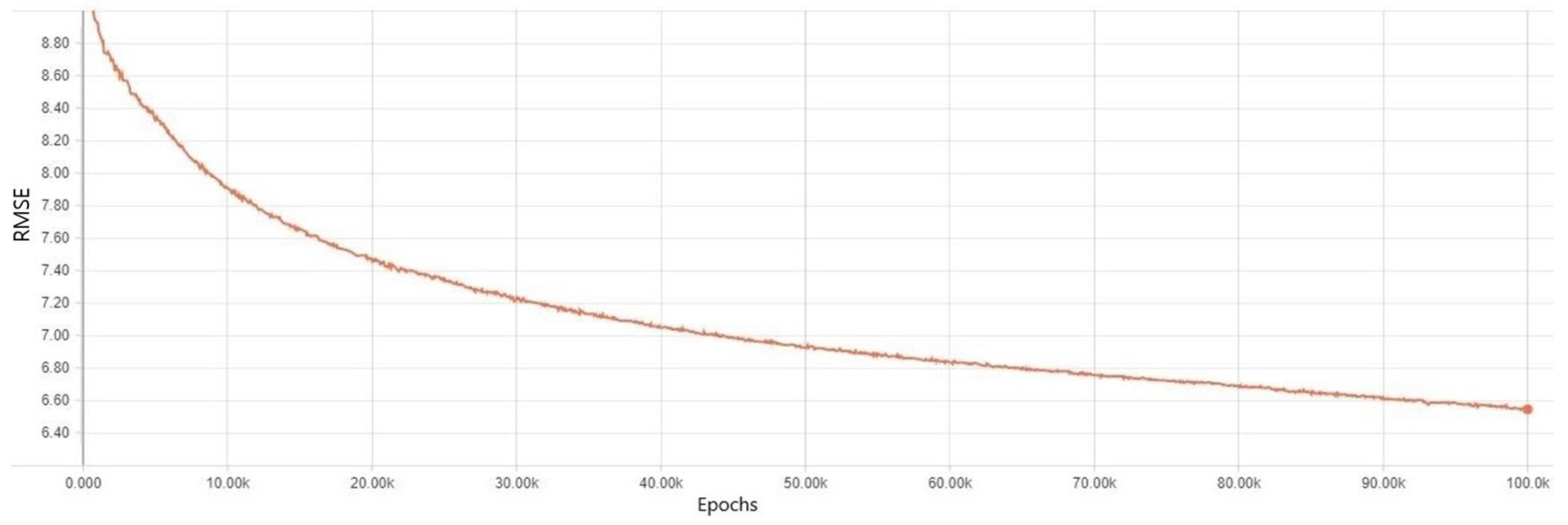
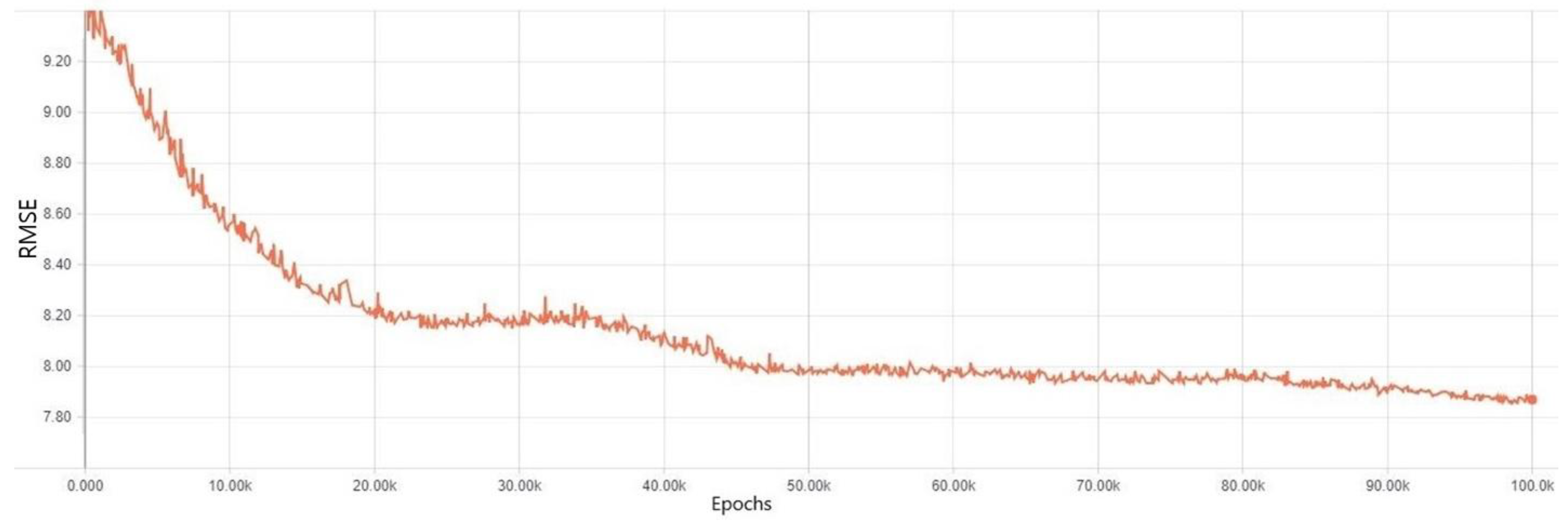
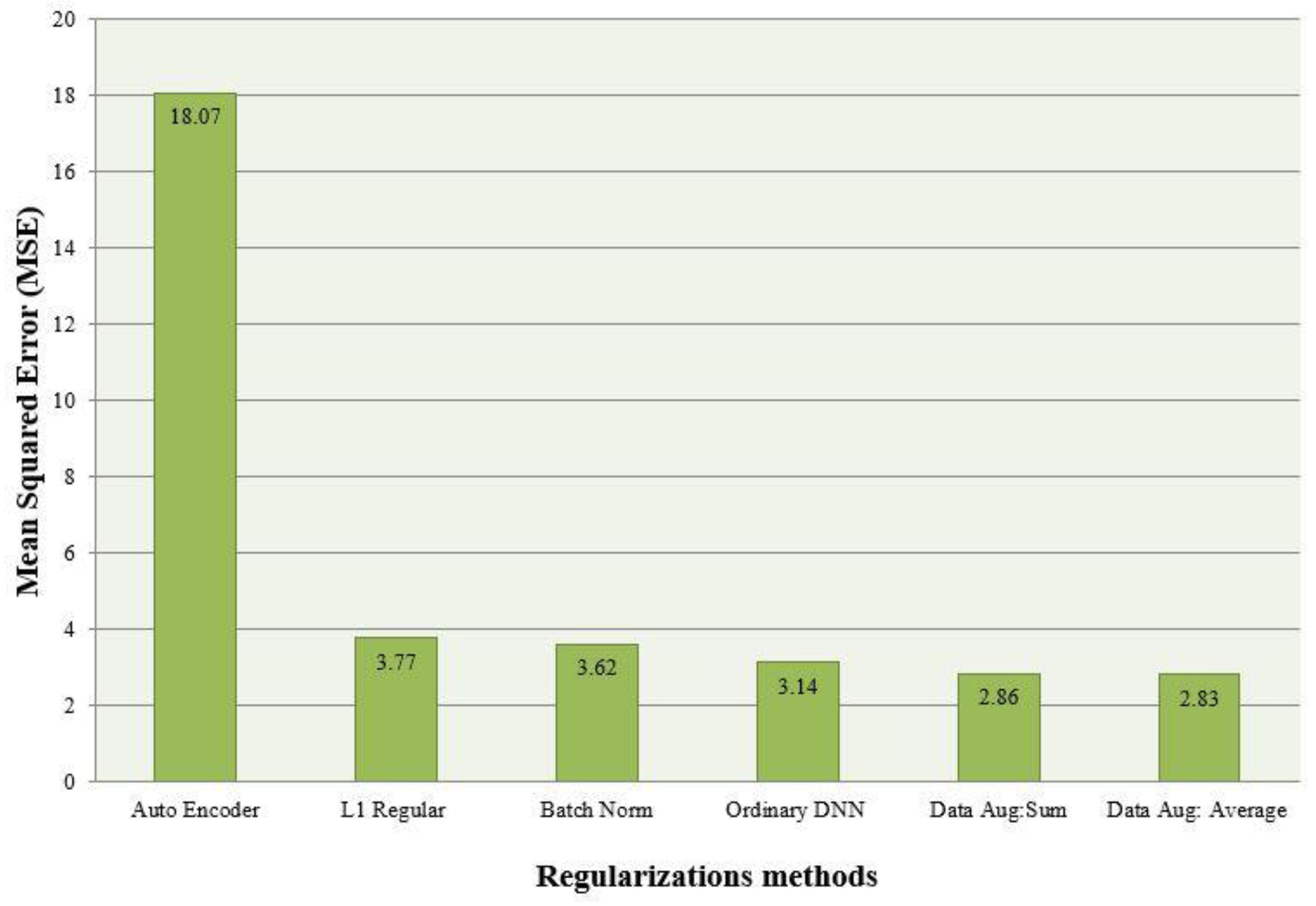
Sometimes, when using DNNRegressor class, all techniques of regularization were not available. For example, for L1 and autoencoder, we had to use another type of API. To do that, we used Keras open source neural network library, which is written in Python. As it can run on top of TensorFlow, it was easy to implement these two libraries together.

For visualization, we used the TensorBoard visualization tool, which is a very powerful graph visualization released by Google’s TensorFlow team. This tool is not only used for graph visualization, but also implemented to plot quantitative metrics on the execution of a graph and to show additional data (e.g., images) that pass through it. Moreover, using this tool, a programmer can debug a model easily. Another API applied for visualization in this research was Matplotlib plotting library. This API provides extremely wide visualization techniques for Python programming language.

3. Results

This chapter discusses the results. First, the results of the DNN model are described, which was trained without the use of any regularization techniques. Next, the results of the DNN models with regularization techniques are presented. Since overfitting problems are much more visible in pictures, our final results are visualized as graphs. The axes of the graphs consist of error values and epoch numbers. Even after training the network model, very low RMSE values seemed to be very good accuracy. However, in some cases, they caused issues such as an overfitting problem.

We first present the experiment results of a DNN without regularization. As previously discussed, our model was established with the settings that are shown in Table 1. After training 100,000 epochs, RMSEs for training and validation data were plotted, as shown in Figure 4 and Figure 5, respectively. Figure 4 shows that, by increasing the epochs, the error for training data changed rapidly. However, the overall training errors decreased.

By comparing the results, we concluded that the errors for validation and training data decreased in the same range. The closeness between the validation and training data errors meant that good generalization was achieved. In some cases, it showed that the neural network model needed more training. However, since it was time-consuming, we continued our research by implementing regularization methods based on this model.

Experiment Results for Each Regularization Method

First, a model where the autoencoder method was applied with the same settings was tested. The results of the training errors are illustrated in Figure 6 and Figure 7. As can be seen from Figure 6, the training errors did not increase as epoch number increased. However, validation errors became higher when the epoch number increased, as illustrated in Figure 7. Through the results, it is clearly seen from the graphs that the model suffered from an underfitting problem and could not learn anything. When we conducted an experiment several times using an autoencoder, the results were not so good. Thus, we could not continue learning. In our analysis, the basic model of stacked encoder was not appropriate. It needed some changes of structure.

Second, we investigated the experiment results of the DNN model, where a batch normalization method was applied. The results of this technique are given in Figure 8 and Figure 9. As it is shown in the figures, the results were more acceptable than those using the autoencoder. The training errors began to decrease initially. However, the overall trend fluctuated constantly after approximately 3000 epochs. Validation errors decreased and increased from the beginning. Even though there was a small decrease around 10,000 epochs, the overall trend increased slightly. By comparing these two graphs, it became clear that the DNN model using batch normalization was overfitted within a small range, because validation errors increased in spite of the constant fluctuation in training errors.

Next, we discuss the DNN model where a L1 regularization method was applied. The experiment results are represented in Figure 10 and Figure 11. Figure 10 shows that the training errors were smoothly diminished as the epoch number increased. However, for validation errors, the trend showed a rise from the beginning of the epochs. This demonstrates that even though the L1 regularization technique was the most popular model to prevent overfitting in artificial intelligence, it still suffered from an overfitting problem.

In reality, a failure occurred during the experiments for all three types of regularization techniques. However, the cause of the failures was undetermined.

Fourth, the experiment results were investigated using data augmentation. As previously discussed, we implemented two types of data augmentation for our investigation. The first scheme, which summed the features, performed better than other regularization methods. As shown in Figure 12 and Figure 13, the training errors simultaneously declined as the number of epochs increased. The validation error of the model found its optimal value at 40K epochs. The validation data error rose slightly after 40K epochs. From these graphs, it is shown that the DNN model with data augmentation based on summing had a slight overfitting after 40K epochs.

Fifth, experiment results using the data augmentation technique based on an average are illustrated in Figure 14 and Figure 15. The figures show that the overfitting issue was completely overcome with this method. As is shown in Figure 14, training errors were considerably diminished throughout all the epochs. For the validation errors, those rapidly decreased until 20K epochs and stayed stable after the point shown in Figure 15. Then, the validation errors began to fall down slowly from 35K epochs, and it showed the smallest error at 100K epochs. Notice the difference between training and validation errors were not high. This indicates that the dataset achieved good generalization.

Next, we compared the accuracies of each scheme by evaluating the averaged mean square errors (MSEs) between estimated temperature and observed temperature. Statistically, the MSE is regarded as an important metric that is used in order to evaluate the performance of a predictor. By comparing the values, we could evaluate the precision and accuracy of predictors. The formula is given below:

$$\mathrm{MSE}=\frac{1}{n}{\sum }_{k=1}^n{(\overline{X_k}-X_k)}^2.$$

(13)

The statistical results are represented in Figure 16.

As it is shown in the figure, the autoencoder scheme was fairly high. For the other schemes, the values were not high. From the results, L1 regularization and the autoencoder still encountered overfitting and underfitting problems. The batch normalization showed better performance than these methods, as mentioned earlier. The DNN model with data augmentation showed the best performance.

Finally, we compared actual average temperature and predicted average temperature in all models. The prediction was done during ten days, from 2018.03.01 until 2018.03.10. The results are shown in

Table 2. Comparison of actual and predicted average temperature.

Date	DNN without Regularization Methods (°C)	L1 Regularization (°C)	Autoencoder (°C)	Data August Sum (°C)	Data August: Average (°C)	Batch Normalization (°C)	Real Temperature (°C)
2018.03.01	2.3	6.3	10.1	1.5	1.0	3.9	4.6
2018.03.02	1.1	−1.9	17.6	−0.2	−0.8	1.0	−0.7
2018.03.03	2.9	−0.5	15.8	0.5	1.4	2.8	7.9
2018.03.04	3.5	17.1	15.1	1.9	0.6	10.3	9.8
2018.03.05	9.3	3.7	10.6	0.7	1.4	16.6	5.5
2018.03.06	4.3	2.7	17.7	4.8	4.5	−0.1	4.5
2018.03.07	2.6	4.4	17.6	8.3	9.1	9.4	6.4
2018.03.08	3.1	7.2	15.2	12.4	7.8	5.6	4.6
2018.03.09	6.6	3.1	16.6	2.7	4.7	4.0	4.5
2018.03.10	1.4	6.1	18.8	4.3	4.9	4.9	4.6

. As can be seen from the table, the scheme that showed the worst performance was the autoencoder because there was much difference between actuality and prediction. For data augmentation and batch normalization, the differences were fairly small. Sometimes, batch normalization outperformed data augmentation during some days. From the table, we see that the data augmentation showed the best performance because the prediction was nearly the same as the real temperature for some days.

4. Discussion

The study showed that the models using regularization techniques demonstrated better performance than those without regularization methods in terms of training errors. When comparing each scheme quantitatively, an autoencoder scheme exposed higher errors than other schemes. This was because it encountered underfitting due to the lack of data caused by removing some of the training data. With this result, the portion of removed data must be decreased for an autoencoder when the training data are insufficient. In addition, L1 regularization and the autoencoder scheme still encountered overfitting and underfitting. Batch normalization and data augmentation showed better performance than the others when comparing the errors. When comparing the prediction accuracy, data augmentation and batch normalization showed better performance than others. Of the two schemes, batch normalization outperformed data augmentation on some days. This was because much more training data was added to the original data instead of being removed. However, if too much data was used for training, it required too much time to complete the training of the models, demonstrating a tradeoff between training data and processing time. In our study, only one CPU was used to train the neural network. If there was too much data, the training time was too long. In future work, it is necessary to analyze how the training time varies and compare the results using big data. One of the approaches to considerably decrease the training time is to use a compute unified device architecture (CUDA) GPU, where the experimental data are stored in a distributed manner and processed in parallel on a multiple-CPU computer. However, this scheme requires the installation of proprietary applications and software. It also requires a change in the basic architecture of the experimental software.

5. Conclusions

The main contribution of this work is to help developers to choose the most suitable scheme for their neural network application by doing comparative research with the purpose of assessing the training and validation errors of a model with regularization methods. In the existing research in the literature of neural networks, there was no research about a comparison of regularization methods. From our study, we see that regularization methods could solve overfitting and underfitting problems efficiently, but, even though some regularization algorithms were applied, neural network models still suffered from the same problems during training. This indicates that it is not easy to solve the problems and a more enhanced solution needs to be devised to completely solve the problems. One remaining aspect to reflect upon consists of a comparison of processing times for each regularization scheme. For stacked autoencoders, it takes a longer time to finish training and validation. The reason for this is not analyzed clearly yet.

References

1. McCulloch, W.S.; Pitts, W. A Logical calculus of the ideas immanent in nervous activity. Bull. Math. Biophys. 1943, 5, 115–133. [Google Scholar] [CrossRef]
2. William, A.A. On the Efficiency of Learning Machines. IEEE Trans. on Syst. Sci. Cybern. 1967, 3, 111–116. [Google Scholar]
3. Nicholas, V.F. Some New Approaches to Machine Learning. IEEE Trans. Syst. Sci. Cybern. 1969, 5, 173–182. [Google Scholar]
4. Zhang, W.; Li, C.; Huang, T.; He, X. Synchronization of Memristor-Based Coupling Recurrent Neural Networks With Time-Varying Delays and Impulses. IEEE Trans. Neural Netw. Learn. Syst. 2015, 26, 3308–3313. [Google Scholar] [CrossRef] [PubMed]
5. Isomura, T. A Measure of Information Available for Inference. Entropy 2018, 20, 512. [Google Scholar] [CrossRef]
6. Elusaí Millán-Ocampo, D.; Parrales-Bahena, A.; González-Rodríguez, J.G.; Silva-Martínez, S.; Porcayo-Calderón, J.; Hernández-Pérez, J.A. Modelling of Behavior for Inhibition Corrosion of Bronze Using Artificial Neural Network (ANN). Entropy 2018, 20, 409. [Google Scholar] [CrossRef]
7. Jian, C.L.; Zhang, Y.; Yunxia, L. Non-Divergence of Stochastic Discrete Time Algorithms for PCA Neural Networks. IEEE Trans. Neural Netw. Learn. Syst. 2015, 26, 394–399. [Google Scholar]
8. Yin, Y.; Wang, L.; Gelenbe, E. Multi-layer neural networks for quality of service oriented server-state classification in cloud servers. In Proceedings of the 2017 International Joint Conference on Neural Networks (IJCNN), Anchorage, AK, USA, 14–19 May 2017. [Google Scholar]
9. Srivastava, N.; Geoffrey, H.; Alex, K.; Ilya, S.; Ruslan, S. Dropout: A simple way to prevent neural networks from over-fitting. J. Mach. Learn. Res. 2014, 15, 1929–1958. [Google Scholar]
10. Suksri, S.; Warangkhana, K. Neural Network training model for weather forecasting using Fireworks Algorithm. In Proceedings of the 2016 International Computer Science and Engineering Conference (ICSEC), Chiang Mai, Thailand, 14–17 December 2016. [Google Scholar]
11. Abdelhadi, L.; Abdelkader, B. Over-fitting avoidance in probabilistic neural networks. In Proceedings of the 2015 World Congress on Information Technology and Computer Applications (WCITCA), Hammamet, Tunisia, 11–13 June 2015. [Google Scholar]
12. Singh, S.; Pankaj, B.; Jasmeen, G. Time series-based temperature prediction using back propagation with genetic algorithm technique. Int. J. Comput. Sci. Issues 2011, 8, 293–304. [Google Scholar]
13. Abhishek, K. Weather forecasting model using artificial neural network. Procedia Tech. 2012, 4, 311–318. [Google Scholar] [CrossRef]
14. Prasanta, R.J. Weather forecasting using artificial neural networks and data mining techniques. IJITR 2015, 3, 2534–2539. [Google Scholar]
15. Smith, B.A.; Ronald, W.M.; Gerrit, H. Improving air temperature prediction with artificial neural networks. Int. J. Comput. Intell. 2006, 3, 179–186. [Google Scholar]
16. Zhang, S.; Hou, Y.; Wang, B.; Song, D. Regularizing Neural Networks via Retaining Confident Connections. Entropy 2017, 19, 313. [Google Scholar] [CrossRef]
17. Kaur, A.; Sharma, J.K.; Sunil, A. Artificial neural networks in forecasting maximum and minimum relative humidity. Int. J. Comput. Sci. Netw Secur. 2011, 11, 197–199. [Google Scholar]
18. Alemu, H.Z.; Wu, W.; Zhao, J. Feedforward Neural Networks with a Hidden Layer Regularization Method. Symmetry 2018, 10, 525. [Google Scholar] [CrossRef]
19. Tibshirani, R. Regression shrinkage and selection via the lasso: A retrospective. Royal Stat. Soc. 2011, 73, 273–282. [Google Scholar] [CrossRef]
20. Hung, N.Q. An artificial neural network model for rainfall forecasting in Bangkok, Thailand. Hydrol. Earth Syst. Sci. 2009, 13, 1413–1425. [Google Scholar] [CrossRef] [Green Version]
21. Chattopadhyay, S. Feed forward Artificial Neural Network model to predict the average summer-monsoon rainfall in India. Acta Geophys. 2007, 55, 369–382. [Google Scholar] [CrossRef] [Green Version]
22. Khajure, S.; Mohod, S.W. Future weather forecasting using soft computing techniques. Procedia Comput. Sci. 2016, 78, 402–407. [Google Scholar] [CrossRef]
23. Cui, X.; Goel, V.; Kingabury, B. Data augmentation for deep neural network acoustic modeling. IEEE/ACM Trans. Audio Speech Lang. Process. 2015, 23, 1469–1477. [Google Scholar]
24. Zhang, H.; Wang, Z.; Liu, D. A Comprehensive Review of Stability Analysis of Continuous-Time Recurrent Neural Networks. IEEE Trans. Neural Netw. Learn. Syst. 2014, 25, 1229–1262. [Google Scholar] [CrossRef]
25. Zhang, S.; Xia, Y.; Wang, J. A Complex-Valued Projection Neural Network for Constrained Optimization of Real Functions in Complex Variables. IEEE Trans. Neural Netw. Learn. Syst. 2015, 26, 3227–3238. [Google Scholar] [CrossRef] [PubMed]
26. Takashi, M.; Hiroyuki, T. An Asynchronous Recurrent Network of Cellular Automaton-Based Neurons and Its Reproduction of Spiking Neural Network Activities. IEEE Trans. Neural Netw. Learn. Syst. 2016, 27, 836–852. [Google Scholar]
27. Hayati, M.; Zahra, M. Application of artificial neural networks for temperature forecasting. Int. J. Electr. Comput. Eng. 2007, 1, 662–666. [Google Scholar]
28. Cao, W.; Yuan, J.; He, Z.; Zhang, Z. Fast Deep Neural Networks With Knowledge Guided Training and Predicted Regions of Interests for Real-Time Video Object Detection. IEEE Acc. 2018, 6, 8990–8999. [Google Scholar] [CrossRef]
29. Wang, X.; Ma, H.; Chen, X.; You, S. Edge Preserving and Multi-Scale Contextual Neural Network for Salient Object Detection. IEEE Trans. Image Process. 2018, 27, 121–134. [Google Scholar] [CrossRef] [PubMed] [Green Version]
30. Yue, S.; Rind, F.C. Collision detection in complex dynamic scenes using an LGMD-based visual neural network with feature enhancement. IEEE Trans. Neural Netw. 2006, 17, 705–716. [Google Scholar] [PubMed]
31. Huang, S.-C.; Chen, B.-H. Highly Accurate Moving Object Detection in Variable Bit Rate Video-Based Traffic Monitoring Systems. IEEE Trans. Neural Netw. Learn. Syst. 2013, 24, 1920–1931. [Google Scholar] [CrossRef] [PubMed]
32. Akcay, S.; Kundegorski, M.E.; Willcocks, C.G.; Breckon, T.P. Using Deep Convolutional Neural Network Architectures for Object Classification and Detection Within X-Ray Baggage Security Imagery. IEEE Trans. Inf. Forensic. Secur. 2018, 13, 2203–2215. [Google Scholar] [CrossRef] [Green Version]
33. Sevo, I.; Avramovic, A. Convolutional Neural Network Based Automatic Object Detection on Aerial Images. IEEE Geo. Remote Sens. Lett. 2016, 13, 740–744. [Google Scholar] [CrossRef]
34. Woźniak, M.; Połap, D. Object detection and recognition via clustered features. Neurocomputing 2018, 320, 76–84. [Google Scholar] [CrossRef]
35. Vieira, S.; Pinaya, W.H.L.; Mechelli, A. Using deep learning to investigate the neuroimaging correlates of psychiatric and neurological disorders: Methods and applications. Neurosci. Biobehav. Rev. 2017, 74, 58–75. [Google Scholar] [CrossRef] [PubMed]
36. Połap, D.; Winnicka, A.; Serwata, K.; Kęsik, K.; Woźniak, M. An Intelligent System for Monitoring Skin Diseases. Sensors 2018, 18, 2552. [Google Scholar] [CrossRef]
37. Heaton, J.B.; Polson, N.G.; Witte, J.H. Deep learning for finance: Deep portfolios. Appl. Stochastic Models Bus. Ind. 2016, 33. [Google Scholar] [CrossRef]
38. Woźniak, M.; Połap, D.; Capizzi, G.; Sciuto, G.L.; Kośmider, L.; Frankiewicz, K. Small lung nodules detection based on local variance analysis and probabilistic neural network. Compt. Methods Programs Biomed. 2018, 161, 173–180. [Google Scholar] [CrossRef] [PubMed]
39. Litjens, G.; Kooi, T.; Bejnordi, B.E.; Setio, A.A.A.; Ciompi, F.; Ghafoorian, M.; Laak, J.A.W.M.; Ginneken, B.v.; Sánchez, C.I. A survey on deep learning in medical image analysis. Med. Image Anal. 2017, 42, 60–88. [Google Scholar] [CrossRef] [PubMed] [Green Version]
40. Woźniak, M.; Połap, D. Adaptive neuro-heuristic hybrid model for fruit peel defects detection. Neural Netw. 2018, 98, 16–33. [Google Scholar] [CrossRef] [PubMed]
41. Wang, J.; Ma, Y.; Zhang, L.; Gao, R.X.; Wu, D. Deep learning for smart manufacturing: Methods and applications. J. Manuf. Syst. 2018, 48, 144–156. [Google Scholar] [CrossRef]
42. Mariel, A.-P.; Amadeo, A.C.; Isaac, C. Adaptive Identifier for Uncertain Complex Nonlinear Systems Based on Continuous Neural Networks. IEEE Trans. Neural Netw. Learn. 2014, 25, 483–494. [Google Scholar]
43. Chang, C.H. Deep and Shallow Architecture of Multilayer Neural Networks. IEEE Trans. Neural Netw. Learn. 2015, 26, 2477–2486. [Google Scholar] [CrossRef] [PubMed]
44. Tycho, M.S.; Pedro, A.M.M.; Murray, S. The Partial Information Decomposition of Generative Neural Network Models. Entropy 2017, 19, 474. [Google Scholar] [CrossRef]
45. Xin, W.; Yuanchao, L.; Ming, L.; Chengjie, S.; Xiaolong, W. Understanding Gating Operations in Recurrent Neural Networks through Opinion Expression Extraction. Entropy 2016, 18, 294. [Google Scholar] [CrossRef]
46. Sitian, Q.; Xiaoping, X. A Two-Layer Recurrent Neural Network for Nonsmooth Convex Optimization Problems. IEEE Trans. Neural Netw. Learn. 2015, 26, 1149–1160. [Google Scholar] [CrossRef] [PubMed]
47. Saman, R.; Bryan, A. A New Formulation for Feedforward Neural Networks. IEEE Trans. Neural Netw. Learn. 2011, 22, 1588–1598. [Google Scholar]
48. Nan, Z. Study on the prediction of energy demand based on master slave neural network. In Proceedings of the 2016 IEEE Information Technology, Networking, Electronic and Automation Control Conference, Chongqing, China, 20–22 May 2016. [Google Scholar]
49. Feng, L.; Jacek, M.Z.; Yan, L.; Wei, W. Input Layer Regularization of Multilayer Feedforward Neural Networks. IEEE Access 2017, 5, 10979–10985. [Google Scholar]
50. Armen, A. SoftTarget Regularization: An Effective Technique to Reduce Over-Fitting in Neural Networks. In Proceedings of the 2017 3rd IEEE International Conference on Cybernetics (CYBCONF), Exeter, UK, 21–23 June 2017. [Google Scholar]
Figure 1. A methodology for the comparative research.
Symmetry 10 00648 g001
Figure 2. The neural network model applied in the experiment.
Symmetry 10 00648 g002
Figure 3. Structure of autoencoder applied in the experiment.
Symmetry 10 00648 g003
Figure 4. Training error results in a deep neural network (DNN) without regularization methods.
Symmetry 10 00648 g004
Figure 5. Validation error results in a DNN without regularization methods.
Symmetry 10 00648 g005
Figure 6. Training mean square errors (MSEs) results in a DNN model for which an autoencoder regularization method was applied.
Symmetry 10 00648 g006
Figure 7. Validation mean square errors results in a DNN model for which an autoencoder regularization method was applied.
Symmetry 10 00648 g007
Figure 8. Training mean square errors results in a DNN model where a batch normalization method was applied.
Symmetry 10 00648 g008
Figure 9. Validation mean square errors results in a DNN model where a batch normalization method was applied.
Symmetry 10 00648 g009
Figure 10. Training error results in a DNN model where an L1 regularization method was applied.
Symmetry 10 00648 g010
Figure 11. Validation error results in a DNN model where an L1 regularization method was applied.
Symmetry 10 00648 g011
Figure 12. Training error results in a DNN model where a data augmentation technique was applied.
Symmetry 10 00648 g012
Figure 13. Training error results in a DNN model where a data augmentation method was applied that summed identical categorical input features.
Symmetry 10 00648 g013
Figure 14. Training error results in a DNN model where a data augmentation method was applied. Taking the average values of the same categorical features was applied.
Symmetry 10 00648 g014
Figure 15. Validation error results in a DNN model where a data augmentation method was applied. Taking the average values of the same categorical features was applied.
Symmetry 10 00648 g015
Figure 16. Comparison of average mean squared error for each regularization method.
Symmetry 10 00648 g016