Online Road Detection under a Shadowy Traffic Image Using a Learning-Based Illumination-Independent Image


School of Electronic and Control Engineering, Chang’an University, Xi’an 710064, China
*
Authors to whom correspondence should be addressed.
Symmetry 2018, 10(12), 707; https://doi.org/10.3390/sym10120707
Submission received: 15 November 2018
/
Revised: 30 November 2018
/
Accepted: 30 November 2018
/
Published: 3 December 2018
Abstract
:Shadows and normal light illumination and road and non-road areas are two pairs of contradictory symmetrical individuals. To achieve accurate road detection, it is necessary to remove interference caused by uneven illumination, such as shadows. This paper proposes a road detection algorithm based on a learning and illumination-independent image to solve the following problems: First, most road detection methods are sensitive to variation of illumination. Second, with traditional road detection methods based on illumination invariability, it is difficult to determine the calibration angle of the camera axis, and the sampling of road samples can be distorted. The proposed method contains three stages: The establishment of a classifier, the online capturing of an illumination-independent image, and the road detection. During the establishment of a classifier, a support vector machine (SVM) classifier for the road block is generated through training with the multi-feature fusion method. During the online capturing of an illumination-independent image, the road interest region is obtained by using a cascaded Hough transform parameterized by a parallel coordinate system. Five road blocks are obtained through the SVM classifier, and the RGB (Red, Green, Blue) space of the combined road blocks is converted to a geometric mean log chromatic space. Next, the camera axis calibration angle for each frame is determined according to the Shannon entropy so that the illumination-independent image of the respective frame is obtained. During the road detection, road sample points are extracted with the random sampling method. A confidence interval classifier of the road is established, which could separate a road from its background. This paper is based on public datasets and video sequences, which records roads of Chinese cities, suburbs, and schools in different traffic scenes. The author compares the method proposed in this paper with other sound video-based road detection methods and the results show that the method proposed in this paper can achieve a desired detection result with high quality and robustness. Meanwhile, the whole detection system can meet the real-time processing requirement.
1. Introduction
Road detection based on vision in the advanced driving assisted system is an important and challengeable task [1]. The vision data can provide abundant information about the driving scenes [2], provide an explicit route plan, and can gain both obstacle detection and road profile estimate information precisely. Therefore, the systems that are vision-based have huge potential in complex road detection scenes [3].
In recent years, road detection has been extensively studied as a key part of automated driving systems, especially in vision-based road detection [4,5,6,7]. Kong et al. [8] applied the vanishing point detection algorithm to road detection, using the Gabor filter to obtain the pixel texture orientation, and the vanishing point position estimation algorithm of an adaptive soft voting scheme and the road region segmentation algorithm with a vanishing point constraint were proposed. Munajat et al. [9] proposed a road detection algorithm based on an RGB histogram filtering and boundary classifier. The RGB image horizontal projection histogram was used to obtain the approximate area of the road, and the cubic spline interpolation was used to obtain the road boundary, which was combined to obtain the road detection result. Somawirata et al. [10] proposed a road detection algorithm that combined the color space and cluster connecting. The color space was used to obtain the initial road area, and the wrong road area was removed by cluster connecting to achieve accurate road detection. Lu et al. [11] proposed a layer-based road detection method, which used the multipopulation genetic algorithm to realize road vanishing point detection, fused vanishing point, and the clustering strategy at the super pixel level to realize road seed point selection; used the GrowCut algorithm to obtain the initial road contour, and used the conditional random field model correction to obtain accurate road detection results. Wang et al. [12] proposed a road detection algorithm based on parallel edge features and a fast road rough segmentation method based on edge connection, and comprehensively applied the parallel edge and road location information, achieving road detection. Yang et al. [13] proposed a road detection algorithm that combined image edge and region features, and used the custom difference operator and region growing method to obtain the edge and region features of the image, respectively, realizing road detection. However, the above studies did not fully consider the effects of illumination changes and shadows on road detection results. In addition, there is a lack of necessary road datasets with a shaded road as an effective verification. As a result, the detection results are more restrictive.
Nowadays, with the rapid development of deep learning and the maturity of its application fields [14,15], road detection methods based on deep learning have emerged, which have a good detection effect on shaded road surfaces [16,17]. Geng et al. [18] proposed a road detection algorithm combining the convolutional neural network (CNN) and Markov random field (MRF), using simple linear iterative cluster (SLIC) to segment the original image into a super pixel map, training CNN to automatically learn road features to obtain road regions, and using MRF to optimize road detection results. Han et al. [19] proposed a semi-supervised and weakly supervised road detection algorithm based on generative adversarial networks (GANs). For semisupervised road detection, GANs was used directly to train unmarked data to prevent overfitting. For weakly supervised road detection, the road shape was used as an additional restriction for conditional GANs. Unfortunately, most deep learning-based approaches have a high execution time and hardware requirements, and only a few of them are suitable for real-time applications [20]. Therefore, it is not advisable to implement road detection through a deep learning-based approach and apply it to practical applications. So, how to effectively remove the effects of illumination changes and shadows on road detection results and obtain higher detection results?
Based on the above, Alvarez et al. [21] introduced the illumination invariance theory into road detection. Alvarez et al. [21] and Frémont et al. [22] systematically analyzed the application of illumination invariance theory to road detection (II-RD). Du et al. [23] proposed a modified illumination invariant road detection method, which combines illumination invariance and random sampling to realize road detection (MII-RD). the above methods not only can effectively eliminate the influence of illumination changes and shadows on road detection results, but was also not limited by a long execution time and expensive hardware requirements. However, the methods of II-RD and MII-RD simply removed the sky area when obtaining the camera axis calibration angle. The remaining area was mixed with a large number of non-road areas, such as vehicles and vegetation, and the vehicle had large bumps and jitters during driving, which caused obvious errors in the obtained angle, and the road detection results were inaccurate. At the same time, II-RD fixedly sampled nine blocks with 10 × 10 pixel sizes in the safe distance area before the vehicle. This fixed position sampling method lacked the randomness of sample selection. When the fixed position was covered with different degrees of traffic markings, manhole covers, spills, cracks, pits, overhauls, ruts, etc. caused by road defects, the sampling of road samples were invalid, and the road detection results had more error. While MII-RD used a random sampling method to collect road sample sets, however, taking the previous frame detection area of the frame as a reference, a frame detection failure was likely to cause continuous detection errors, and the calculation efficiency was low.
Therefore, in this paper, we propose implementation of an online road detection process on a shaded traffic image using a learned illumination-independent image (OLII-RD). We manually calibrate the road block and non-road block of the image sequence, and use the multi-feature fusion method to obtain the road block and non-road block color information matrix and the gray level co-occurrence matrix feature vector to establish the road block SVM classifier. A cascading Hough transform parameterized by a parallel coordinate system is used to acquire a road region of interest, and blocks of 30 × 30 pixels are randomly extracted from the region of interest. We use the SVM classifier to determine the five road blocks and combine them, and convert the RGB space of the combined road block into a geometric mean log chromatic space, and determine the camera axis calibration angle for each frame according to Shannon entropy, and then calculate illumination-independent images for the respective frames. The road sample points are extracted by the random sampling method in the safety distance area of the vehicle, and the road confidence interval classifier is established. The final road detection result is obtained by the road confidence interval classifier.
In brief, this paper has three main contributions:
- (1)
- It comes up with a learning-based illuminant invariance method, which greatly solves the influences of the major interference of shadow detection in the road images and gains more accurate, robust road detecting results.
- (2)
- This paper proposes an online road detection method, which avoids partial detection in the offline detection, achieves subtle detection on every shaded frame of the road images, and gains more effective and robust results.
- (3)
- Compared with the advanced methods of II-RD and MII-RD based on common open image sets, by using the methods proposed in this paper, we could gain more precise and robust detecting results. Besides these advantages of this detecting method based on the common open datasets, we can gain the same effective results by using our own images and datasets.
The contents of each part of our paper are as follows. The second part describes theoretical models based on the proposed illuminant invariant image. The third part introduces online learning-based precise capture processing of the theta angle proposed in this paper. The forth part particularly illustrates the accurate steps of the road detecting algorithm proposed in this paper. The fifth part mainly describes the experiments, including datasets, doctrines, compared methods, results, and necessary discussions. The last part summarizes the full text and describes the next research directions and work content.
2. Illumination-Independent Image
The traditional optical sensor model shows that the data acquired by the image acquisition device is the energy result of the spectral power distribution of the light source, the surface reflection of the object, and the imaging of the spectral sensor.
The spectral power distribution is represented by , the surface reflection function is represented by , and the camera sensitization function is represented by . Then, the RGB color image has three channel values:
The in the formula is Lambertian shading [24].
Supposing the camera photoreceptor function, , is a Dirac function [25], i.e., . Then, Formula (1) becomes:
Suppose the illumination approximates the Planckian Rule [24], i.e.:
where and are constants, T is the illumination color, and I is the total illumination intensity.
Approximately, RGB has three channels, (k = R, G, B or k = 1, 2, 3), which can be obtained by Equation (3).
Let be the geometric mean of the three channels, , of the RGB:
Then, the chromaticity is:
After taking the logarithm on both sides:
In the geometric mean log chromaticity space of Equation (7), and are orthogonal (i.e., ), and convert the space into a two-dimensional space using the coordinate system transformation.
where is a two-dimensional column vector, , , .
Thus, the illumination-independent image can be obtained from Equation (9):
where is the camera axis calibration angle.
3. Learning-Based Online Calibration
Ideally, the direction is an inherent parameter of the camera ranging from 1 to 180. It is the presented result on the basis of these three assumptions: a Planckian light, Lambertian surface, and narrow-band sensor [24]. However, there are many limits while using the assumptions because most image sensors are not compatible with a narrow band. Additionally, the value of each image frame is unstable because the camera in the car might be shaking while the car is moving on different road conditions. Therefore, it is necessary to confirm the value of of each image frame online to make sure that each frame of the image is as close as possible to its optimal state.
In this paper, a learning-based method is proposed to determine the of each frame image online. The algorithm flow chart is shown in Figure 1.
3.1. Road Block Feature Extraction with Multi-Feature Fusion
The selected training set image sequence, N, should be big enough to contain different illumination environments, weather conditions, and images under different traffic scenes. We select several parts from each image frame to attain the road parts and the non-road parts, which, respectively, can be considered as the positive sample and negative sample. The feature extraction methods based on the multi-feature fusion proposed in this paper have effectively distinguished between the road parts and the non-road parts by using the feature vector of the color information matrix and gray level co-occurrence matrix.
The color information mainly scatters in low-level matrices. It can validly present the color distribution of images by extracting color information matrices, including color distance, first-level matrices, second-level matrices, and third-level matrices.
Color distance:
Among them, Ci and Cj represent pixel i and pixel j, and R, G, and B correspond to three channels.
First moment:
Second moment:
Third moment:
where is the probability of occurrence of a pixel whose gradation is j in the ith color channel component of the color image, and N represents the number of pixels.
The color information matrix characteristics of the image are expressed as follows:
Except the color feature, the texture feature is also an important part of characterizing object features. Using the gray level co-occurrence matrix to obtain feature descriptions, such as the contrast, energy, entropy, and homogeneity, to describe object texture features [26].
- (1)
- Contrast: Is the measure of how much the local change is in the image, which reflects the sharpness and the texture groove depth of the image. The deeper the texture groove is, the clearer the result is. On the contrary, the contrast value is smaller, then the groove is shallower and the result is more blurred:where i and j represent horizontal and vertical coordinates, and p(i, j) refers to a normalized gray level co-occurrence matrix.
- (2)
- Energy: Is the measure of stability of the image texture grayscale change, which reflects the image distribution uniformity and texture thickness. A high energy value reflects that the current texture change is more stable:
- (3)
- Entropy: Is a measure of the randomness of an image containing the amount of information. It shows the complexity of the gray level distribution of the image. The larger the entropy value, the more complicated the image:
- (4)
- Homogeneity: Is the similarity of the gray level of the image in the row or column direction, reflecting the local gray correlation. The larger the value, the stronger the correlation:where and represent the average of the horizontal and vertical coordinates, respectively, and and represent the average of the horizontal and vertical coordinates, respectively.
The gray level co-occurrence matrix features of the image are expressed as follows:
3.2. SVM Road Block Classifier
SVM was first proposed by Cortes and Vapnik in 1995. It has unique advantages in solving small sample, nonlinear, and high-dimensional pattern recognition. It has good generalization ability and is incomparable to other machine learning [27]. SVM uses the separation hyperplane as a linear function of the separation training data to solve the nonlinear classification problem. The optimization function for obtaining the optimal classification surface is as follows:
In the formula, x is the sample, n is the number of samples, y is the category number, is the Lagrange coefficient when the function is optimized, c is the penalty function, and is the kernel function that satisfies the Mercer condition.
The SVM discriminant function is:
When SVM is used for classification, the key lies in the choice of kernel function, . The parameter optimization related to the kernel function is the key factor affecting the classification effect [28]. The form of the kernel function and the determination of its associated parameters determine the type and complexity of the classifier. At present, the most commonly used kernel functions are linear kernel functions, polynomial kernel functions, radial basis RBF kernel functions, and S-shaped kernel functions. We select the RBF kernel function based on experimental data and experience, and the expression form is:
In the formula, is the bias term, gamma is the parameter, g, of the kernel function, is the number of support vectors, is the coefficient of the support vector, is the support vector, and is the sample to be predicted.
The experimental data of SVM is a matrix composed of rows of feature vectors. In the experiment, the matrix is normalized first, and then Libsvm [29] is used to realize classification. In this paper, we use the method of Section 3.1 to extract the road block and non-road block color information matrix and the gray level co-occurrence matrix as the feature vector for SVM training, and generate the SVM road block classifier.
3.3. Minimum Entropy Solution
In order to obtain the of the road block, the Shannon entropy theorem [24] is introduced in this paper:
where is the entropy value and is the probability that the gray value in the gray histogram falls within the ith bin. The bin-width of the gray histogram is determined by Scott’s law [24]:
where N is the size of the image.
According to the definition of entropy, if there are more bins in the gray histogram, the smaller is, the larger the entropy value is. Therefore, the angle corresponding to the minimum entropy is the angle of the frame image.
4. Road Detection Algorithm
4.1. Region of Interest Extraction
(1) Sky removal
The literature [22] points out that non-sky areas (roads, vehicles, buildings, vegetation, pedestrians, etc.) conform to the Lambert reflection, and the sky area conforms to Rayleigh scattering, and its model is as shown in Equation (25). The log chromaticity of the sky region does not follow the axis calibration theorem:
where represents the intensity of the scattered light, represents the intensity of the incident light, and represents the wave.
At the same time, there are many kinds of road line. According to the type of road longitudinal section, the road line can be divided into parallel road, uphill, and downhill. In the case of uphill and downhill, as Figure 2a,b shows, it might cause the missing road surface area and larger non-road areas by using the sky removal method with a fixed coordinate position to influence the accuracy of the results. Therefore, we propose to use the cascaded Hough transform method based on parallel coordinate system parameterization proposed in this paper to obtain the vanishing point of the road [30]. Firstly, we use the cascaded-Hough transform algorithm to transform originally infinite space into a limited diamond space. Then, we rasterize the space, and use the voting method to find the vanishing point. After the vanishing point is determined, the horizontal line where it is located is the horizon position sought, and the area below the horizon in the image is the area of interest for road detection.
(2) Hood removal
Due to problems, such as the camera erection position and camera shooting angle, the actual collected traffic road image often has a hood. The hood occupies the road area in the image and later interferes with the selection of road sampling points in Section 4.3, which in turn affects the detection of the road. Considering that the camera erection position is relatively fixed, we use the manual calibration method to remove the front part, as shown in Figure 2b,c. The specific steps are as follows:
- (1)
- Determining different road image data sets Seq1, Seq2, …, Seqn;
- (2)
- Randomly extract 20 frames from the dataset Seq1, calculate the head position Dis(i), i = 1, 2, ..., 20, and calculate the Dis(i) mean value to determine the final split position, Dis_head;
- (3)
- Mark the video sequence according to the calculated Dis_head to remove the hood area of the vehicle; and
- (4)
- Repeat steps (2) and (3) for data sets, Seq2, … , Seqn.
4.2. Illumination-Independent Image Acquisition
Obtaining the angle of the road image of each frame online is the basis for obtaining the illumination-independent image and realizing road surface detection. We propose to randomly select three 30 × 30 area blocks in the region of interest, and calculate the eigenvalues corresponding to the color information matrix and the gray level co-occurrence matrix. The road block classifier established in Section 3.2 determines whether it is a road block, and then calculates the of the road block. Finally, the illumination-independent image of the corresponding frame is obtained by the calculated . A more detailed description of the illumination-independent image acquisition algorithm is presented in Algorithm 1:
| Algorithm 1. Illumination-independent image acquisition |
| Require: Number of road blocks n = 3, color information matrix feature, gray level co-occurrence matrix feature, SVM road block classifier |
| Ensure: Illumination-independent image corresponding to a certain frame |
| 1: for k = first frame do last frame |
| 2: for i = 1 do N (number of blocks, N ≥ 3) |
| 3: Randomly extract a block of 30 × 30 pixel, and n = 1; |
| 4: Extract the region block feature color information matrix, gray level co-occurrence matrix and input its into the SVM road block classifier; |
| 5: if road block then |
| 6: Store road blocks in a 150 × 30 matrix, and n = n + 1; |
| 7: else |
| 8: i = i + 1, Repeat steps 3~6; |
| 9: end if |
| 10: Compose new image with 90 × 30 pixels; 11: Calculate the new image online angle by the minimum entropy algorithm; |
| 12: Obtain the illumination-independent image using the illumination-independent image theory; |
| 13: end for |
| 14: end for |
The illumination-independent image obtained by the learning method is shown in Figure 3:
4.3. Road Sample Set
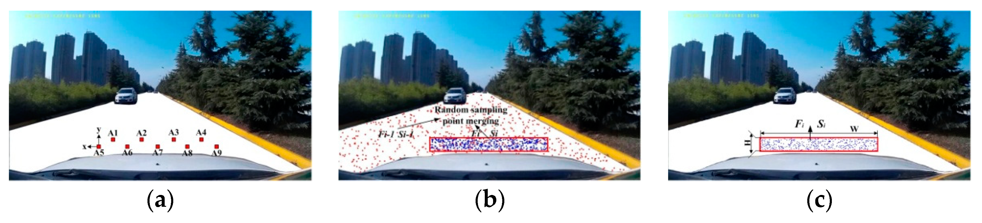
Choosing the appropriate road sampling method is an important part of extracting road features, constructing road models, establishing confidence intervals, and determining road areas. II-RD samples nine sample areas of a 10 × 10 pixel size at a fixed position in the safety distance area of the vehicle, as shown in Figure 4a. For MII-RD, based on the safety distance area in front of the vehicle in the current frame, the road detection area of the previous frame is used as a reference to determine the current frame sampling set, as shown in Figure 4b. However, we propose that 900 sampling points are randomly selected based on the safe distance field in front of the vehicle in the frame (current frame), as shown in Figure 4c.
To clearly describe the sampling method of our method (OLII-RD), the following mathematical symbols are defined:
represents the ith frame image in the video, and represents the frame road sample set. N is a constant, representing the total number of pixels in the road sample area of the frame, and n represents the number of road sample points in the frame.
Current frame vehicle safety distance area sample collection. The safety distance area in front of the vehicle is roughly the road area, the size is W × H, and there are N pixels, as shown in Figure 4c. We use this as the road sampling area, and uses the simple random non-return sampling method to extract n sampling points (for a finite population, when , it can be approximated as a simple random sample) as the frame road sampling sets, .
4.4. Road Classifier
In this paper, the normal distribution model is used to fit the road sample set, and the road confidence interval classifier is established. Taking 90% of the data in the center of the normal distribution represents the chromaticity characteristics of the road, and the confidence interval, (), of the road is determined by the percentile method. Points with eigenvalues in the range of are road areas, and vice versa are backgrounds or obstacles (such as roads, vehicles, buildings, vegetation, pedestrians, etc.). The road detection confidence interval classifier is defined as:
5. Experimental Results
In this chapter, we use several experiments to evaluate the performance of the road detection system proposed in this paper. Under different illuminating conditions, weather conditions, and traffic scenes, we test several moving-vehicle video sequences captured on city streets and suburban roads. In order to further evaluate the performances of our system, we also compare our method with other state of art methods with II-RD [21] and MII-RD [23]. The reason why we chose II-RD [21] and MII-RD [23] is that we have our considerations. II-RD [21] introduced illumination invariance theory into road detection, and systematically analyzed the application of illumination invariance theory to road detection. As the first systematic argumentation analysis, the importance of II-RD [21] is self-evident. MII-RD [23] proposed a modified illumination invariant road detection method, and it is also the latest research results, so timeliness is guaranteed. The method proposed by us is also related to the theory of illumination invariance, so we chose to compare II-RD [21] and MII-RD [23], which are most closely related to the theory and application of illumination invariance and best reflect the advantages of the proposed method.
5.1. The Experiment of the CVC Public Dataset
The experimental image set uses the common dataset, CVC [21], which contains a large number of road video image sequences. The sequence is acquired by an onboard camera based on the Sony ICX084 sensor. The camera is equipped with a microlens with a focal length of 6 mm and an image frame acquisition rate of 15 fps.
The experiment uses three different image sequences among them. The first image sequence, SS, contains 350 frames of different scene road images for road block feature extraction and SVM road block classifier training. The second sequence of images, dry road sequence (DS), includes 450 images of sunny shadows, supporting the presence of shadows. The third sequence of images, rainy road sequence (RS), consists of 250 images, which are road images after the rain and the road is wet. The resolution of the three image sequences is 640 × 480, and each pixel is 8 bits. The DS and RS sequences are dry and wet environment road pavements with various forms and complicated scenes, and the vehicles are driving on the road.
Public dataset image sequences are available online: http://www.cvc.uab.es/adas/databases/.
5.1.1. Sampling Method Experiment
For II-RD, nine fixed-area, fixed-size (10 × 10) road blocks are collected as sampling points in the safe distance area in front of the vehicle. MII-RD determines that the current frame, , has a size of 250 × 30 area, Si, and randomly selects 500 sampling points from Si, and 400 sampling points are randomly selected from the previous frame, Fi−1, road detection result, Si−1. Finally, a total of 900 sampling points are extracted. However, in this paper, we directly select 900 sampling points from Si.
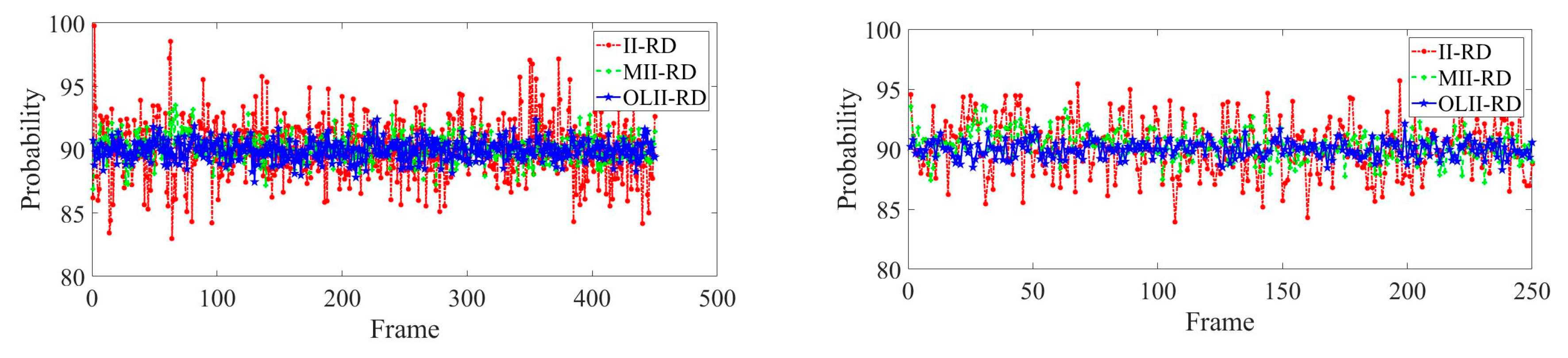
The data collected by II-RD, MII-RD, and OLII-RD are, respectively, fitted with normal distribution, as shown in Figure 5. The sampling method’s error calculation results of II-RD, MII-RD and OLII-RD are shown in Table 1.
It can be seen from Figure 5 and Table 1 that the mean value of our sampling method is closer to 90%, and the sampling standard deviation is significantly lower than for II-RD and MII-RD. For II-RD, the sampling method of the fixed position in the safe distance area in front of the vehicle lacks the randomness of sample selection, and it is easy to sample traffic signs, manhole covers, spills and road defects, cracks, pits, ruts, etc., which causes that road sample to be invalid, and the road detection result has a large error. For MII-RD, the upper and lower frame joint sampling method is adopted, the sampling distribution range is wide, and the probability of collecting non-road surface area is increased. If a frame detection fails, the error of the result is easily expanded. The sampling method proposed by us can effectively avoid the limitations of the fixed position sampling, and can also greatly reduce non-road interference, and can get better and more robust results.
5.1.2. Qualitative Road Detection Result
We systematically test the CVC public datasets. Figure 6 shows some typical detection results of DS and RS video sequences. Among them, 1~3 lines are the detection results of many vehicles on the road; 4~6 lines are the results of the detection of obvious sunlight and road shadows; 7~9 lines are the detection results of irregular road lines and complex scenes. Each line shows the original image, groundtruth map, II-RD detection results, MII-RD detection results, and OLII-RD detection results.
5.1.3. Result Evaluation Index
This paper uses the precision, recall, and comprehensive evaluation index, F, to quantitatively evaluate the road detection results [31].
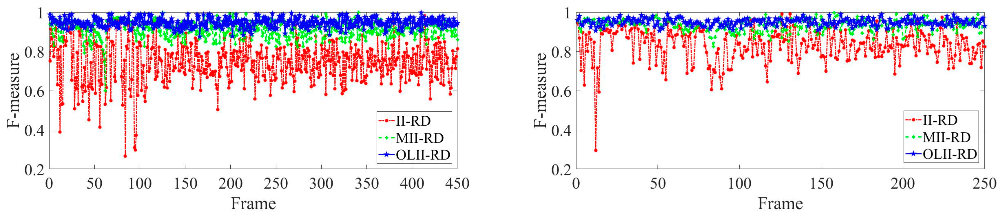
The definition is as follows: ① Accuracy rate, P, ② recall rate, R, ③ comprehensive evaluation index, F. Let be the real area of the road, and be the actual detection result of the road surface, then , , , . P and R are complementary, F is the weighted harmonic average of P and R, and can reconcile and comprehensively reflect the accuracy, P, and the recall rate, R. The closer F is to 1, the better the road detection effect. Because we use the random sampling method, the P, R, F values have slight fluctuations, and the standard deviation of the fluctuation is . The comparison of the performance indexes of the three methods is shown in Table 2. The comprehensive evaluation index, F, curve of the three methods for each frame image detection result is shown in Figure 7.
5.2. The Experiment of the Self-Built Video Sequence
To further illustrate the robustness of our detection system, we also test the road datasets that are taken by our own car outdoors. Similarly, we also compare our method with II-RD and MII-RD on these self-built datasets.
The test video sequence is the actual road dataset of China obtained by the driving recorder, named visual road recognition (VRR). The VRR is shot by the SAST F620 driving recorder. The wide angle is 170° and the frame rate is 30 frames per second. It is mounted on the top of the car about 1.5 m from the road surface. The original resolution is 1920 × 1080. For experimental purposes, the test video sequence selects one frame of the road image every five frames, and the original image of each frame obtained is normalized by downsampling with a resolution of 640 × 360.
Two of the video sequences, Sequence1, Sequence2 (hereinafter referred to as S1, S2), are selected for testing experiments. The sequence, S1, is collected from the Liuxue section of the Weihe River in Xi’an, Shaanxi Province. The video sequence duration is 3 m 9 s, and the effective frame number is 1130 frames. The road is a two-way two-lane road, the road video is intensely illuminated, the shadow contrast is obvious, and the vehicle passes frequently. S2 is collected from the Mingguang section of Weiyang District, Xi’an City, Shaanxi Province. The video sequence duration is 2 m 25 s and the effective frame number is 870 frames. The road video is dark and the road surface is similar to the surrounding features.
5.2.1. Qualitative Road Detection Result
We systematically test the self-built VRR datasets. Figure 8 shows some typical detection results for the two video sequences, S1 and S2, where each row shows the comparison detection results of the three detection methods of the same image frame.
5.2.2. Result Evaluation Index
The road detection results are quantitatively evaluated using the same evaluation indicators as in Section 5.1.3, and the precision, recall, and F index of the detection results are calculated. The comparison of the performance of the three methods is shown in Table 3. The index F curve of the results of the three methods of each frame image is shown in Figure 9.
In addition to the two video sequences (S1 and S2) tested above, the remaining five video sequences were also tested. The video sequences, 3 and 4, are captured in a suburban environment, the video sequence, 5, is captured in a school road environment, and the video sequences, 6 and 7, are captured in an urban road environment. We save the detection results on each frame, and after the entire process, calculate the accuracy, recall rate, and comprehensive evaluation index, F. Table 4 lists the details of the datasets and detection results. The results of these detections indicate the overall accuracy and stability of our system.
5.3. The Experiment of the Strong Sunlight and Low Contrast Condition
Illumination change is a challenge in the illumination-independent image acquisition stage and the road detection stage. To improve the robustness of road block selection, more road samples under different lighting conditions are added to the constraints in 3.1. We select 600 frames from the datasets, most of which were taken under strong sunlight or at very low contrast. Some typical results are shown in Figure 10, where each row shows the results of three methods in the same sequence of scenes. The frames in scenes 1, 2 are cases where the reflected light is severe under strong sunlight. The frames in scenes 3 and 4 are when the sunlight is very low in the evening. The frames in scenes 5 and 6 are road scenes taken under noon direct sunlight conditions. The frames in scenes 7, 8 are road scenes taken at very low contrast time in the evening.
5.4. Detection Results Analysis and Discussion
Systematic detections are carried out for II-RD, MII-RD, and OLII-RD in the CVC dataset and self-built video sequence, respectively. For qualitative results, we find that the road detection results by II-RD and MII-RD have large errors, but the results of OLII-RD are more accurate and robust. The results of II-RD are usually incomplete, and there is a large road pavement missing, and the recall rate is the highest. The results of MII-RD are easy to include non-road parts on both sides of the road, and there is a large detection error. For quantitative results, OLII-RD in the accuracy of P, recall rate, R, and comprehensive evaluation index, F, and its stability is better than II-RD and MII-RD; among them, the comprehensive evaluation index, F, can reach more than 90%. Furthermore, under the strong sunlight and low contrast condition, our method still obtains better and more stable results.
Therefore, the road detection effects proposed by us in different lighting environments, different weather conditions, and different traffic scenarios were achieved, and our detection method also had good transplantation ability.
5.5. Time Validity Analysis
In this section, the calculation time of II-RD, MII-RD, and OLII-RD at each stage is calculated. This experiment uses Windows 10 64-bit operating system, CPU is Intel Core i5-4570, 3.2 GHz, 8 G PC as the experimental platform, and the experimental environment is MATLAB 2017b. In this part, the random sampling method is used to randomly extract 100 frames from the public dataset and the self-built dataset for time validity analysis experiments. For the resolution of the image frames of the two data sets, we use clipping and quantization processing to uniformly quantize to 640 × 480.
The road detection method in this paper can be summarized as two processes: Offline training and online detection. For the offline training process, mainly the road block feature extraction and the establishment of the SVM road block classifier, during the actual comparison process, the time consumption of this stage may not be measured. For the online detection process, it can be summarized into four stages: ① Interested region extraction, ② illumination-independent image acquisition, ③ road sample collection and classification, and ④ morphological processing.
With a uniform processing standard, our current implementation is non-optimized MATLAB code. Figure 11 shows the average processing time for each of the three methods in each of the two datasets. II-RD and MII-RD removed the upper third of the image, respectively, and OLII-RD uses the horizon determination algorithm to remove the area above the horizon. It can be seen from the figure that the total processing time of MII-RD is the longest, the time is about 470 ms, and the road sample collection time is relatively long. The least time spent on total time is the method of II-RD, and the time is about 370 ms. The total time consumption of OLII-RD is about 430 ms, which is somewhere in between. Although, the paper uses the online acquisition, , angle and the time consumption in the extraction stage of the region of interest is more than II-RD and MII-RD. However, the obtained road area of interest is more concentrated, and the number of pixels processed is relatively small, which saves more time for the subsequent illumination-independent image acquisition stage.
The experimental results show that the average processing speed of our detection method is about 2.5 fps. According to our experience in similar applications, we think that just by going to C++, this code can easily run in less than 70 ms. In the actual application process, a certain number of interval frames can be selectively selected, and specific real-time requirements can be met without affecting the final results of the experiment.
6. Conclusions
Road detection is a key step in realizing a vehicle’s automatic driving technology, and plays an important role in the rapid development of assisted driving and unmanned driving technology. In this paper, an online road detection method based solely on vision using learning-based illumination-independent image on shadowed traffic images was proposed to solve the effects of illumination changes and shadows on road detection results. We came up with a learning-based illuminant invariance method, which greatly solves the influences of the major interference of shadow detection in the road images. We proposed the online road detection method, which avoided partial detection in the offline detection, achieved subtle detection on every shadowed road image, and gained more effective and robust results. The effectiveness of the proposed method was tested by multiple image sequences under CVC and self-built datasets, including different traffic environments, different road types, different vehicle distributions, and different road scenarios. The F-value of the comprehensive evaluation index in road detection was about 93% on average, which proved the effectiveness of the proposed method. In addition, the entire detection process can meet real-time requirements. In the future, we plan to realize joint detection and classification identification of multiple traffic objects, such as people, vehicles, and roads.
Data Availability
The data used to support the findings of this paper are available from the corresponding author upon request. All data are included within the manuscript.
Author Contributions
Y.S. and Y.J. conceived and designed the experiments; Y.S., K.D. and J.S. presented tools and carried out the data analysis; Y.S. wrote the paper. Y.J., W.L. and J.S. guided and revised the paper. Y.S. rewrote and improved the theoretical part. K.D. and W.L. collected the materials and did a lot of format editing work.
Funding
This research was funded by the General Program of National Natural Science Foundation of China (NSFC) under Grant No. 61603057, No. 11702035 and No. 61803040. This research was also partially supported by the Fundamental Research Funds for the Central Universities under Grant No. 300102328403 and the Shaanxi province Science and Technology Industrial Research Projects under Grant No. 2015GY033.
Acknowledgments
The authors are grateful for the comments and reviews from the reviewers and editors.
Conflicts of Interest
The authors declare no conflict of interest.
References
- Burns, L.D. Sustainable mobility: A vision of our transport future. Nature 2013, 497, 181. [Google Scholar] [CrossRef] [PubMed]
- Islam, K.T.; Raj, R.G.; Mujtaba, G. Recognition of Traffic Sign Based on Bag-of-Words and Artificial Neural Network. Symmetry 2017, 9, 138. [Google Scholar] [CrossRef]
- Sivaraman, S.; Trivedi, M.M. Looking at Vehicles on the Road: A Survey of Vision-Based Vehicle Detection, Tracking, and Behavior Analysis. IEEE Trans. Intell. Transp. Syst. 2013, 14, 1773–1795. [Google Scholar] [CrossRef] [Green Version]
- Xing, Y.; Lv, C.; Chen, L.; Wang, H.; Wang, H.; Cao, D.; Velenis, E.; Wang, F.Y. Advances in Vision-Based Lane Detection: Algorithms, Integration, Assessment, and Perspectives on ACP-Based Parallel Vision. IEEE/CAA J. Autom. Sin. 2018, 5, 645–661. [Google Scholar] [CrossRef]
- Hillel, A.B.; Lerner, R.; Dan, L.; Raz, G. Recent progress in road and lane detection: A survey. Mach. Vis. Appl. 2014, 25, 727–745. [Google Scholar] [CrossRef]
- Mendes, C.C.T.; Frémont, V.; Wolf, D.F. Vision-Based Road Detection using Contextual Blocks. arXiv, 2015; arXiv:1509.01122. [Google Scholar]
- Zhang, Y.; Su, Y.; Yang, J.; Ponce, J.; Kong, H. When Dijkstra Meets Vanishing Point: A Stereo Vision Approach for Road Detection. IEEE Trans. Image Process. 2018, 27, 2176–2188. [Google Scholar] [CrossRef] [Green Version]
- Kong, H.; Audibert, J.Y.; Ponce, J. General road detection from a single image. IEEE Trans. Image Process. 2010, 19, 2211–2220. [Google Scholar] [CrossRef]
- Munajat, M.D.E.; Widyantoro, D.H.; Munir, R. Road detection system based on RGB histogram filterization and boundary classifier. In Proceedings of the International Conference on Advanced Computer Science and Information Systems, Depok, Indonesia, 10–11 October 2015; pp. 195–200. [Google Scholar]
- Somawirata, I.K.; Utaminingrum, F. Road detection based on the color space and cluster connecting. In Proceedings of the IEEE International Conference on Signal and Image Processing, Beijing, China, 13–15 August 2016; pp. 118–122. [Google Scholar]
- Lu, K.; Li, J.; An, X.; He, H. Vision Sensor-Based Road Detection for Field Robot Navigation. Sensors 2015, 15, 29594–29617. [Google Scholar] [CrossRef] [Green Version]
- Wang, W.; Ding, W.; Li, Y.; Yang, S. An Efficient Road Detection Algorithm Based on Parallel Edges. Acta Opt. Sin. 2015, 35, 0715001. [Google Scholar] [CrossRef]
- Yang, T.; Wang, M.; Qin, Y. Road detection algorithm using the edge and region features in images. J. Southeast Univ. 2013, 43, 81–84. [Google Scholar]
- Zhu, D.; Dai, L.; Luo, Y.; Zhang, G.; Shao, X.; Itti, L.; Lu, J. Multi-Scale Adversarial Feature Learning for Saliency Detection. Symmetry 2018, 10, 457. [Google Scholar] [CrossRef]
- Badrinarayanan, V.; Kendall, A.; Cipolla, R. SegNet: A Deep Convolutional Encoder-Decoder Architecture for Scene Segmentation. IEEE Trans. Pattern Anal. Mach. Intell. 2017, 39, 2481–2495. [Google Scholar] [CrossRef]
- Cheng, G.; Wang, Y.; Xu, S.; Wang, H.; Xiang, S.; Pan, C. Automatic Road Detection and Centerline Extraction via Cascaded End-to-End Convolutional Neural Network. IEEE Trans. Geosci. Remote Sens. 2017, 55, 3322–3337. [Google Scholar] [CrossRef]
- Narayan, A.; Tuci, E.; Labrosse, F.; Alkilabi, M.H.M.; Narayan, A.; Tuci, E.; Labrosse, F.; Alkilabi, M.H.M. Road detection using convolutional neural networks. In Proceedings of the European Conference on Artificial Life Ecal, Lyon, France, 4–8 September 2017; pp. 314–321. [Google Scholar]
- Geng, L.; Sun, J.; Xiao, Z.; Zhang, F.; Wu, J. Combining CNN and MRF for Road Detection. Comput. Electr. Eng. 2018, 70, 895–903. [Google Scholar] [CrossRef]
- Han, X.; Lu, J.; Zhao, C.; You, S.; Li, H. Semisupervised and Weakly Supervised Road Detection Based on Generative Adversarial Networks. IEEE Signal Process. Lett. 2018, 25, 551–555. [Google Scholar] [CrossRef]
- Costea, A.D.; Nedevschi, S. Traffic scene segmentation based on boosting over multimodal low, intermediate and high order multi-range channel features. In Proceedings of the Intelligent Vehicles Symposium, Los Angeles, CA, USA, 11–14 June 2017; pp. 74–81. [Google Scholar]
- Alvarez, J.M.Á.; Lopez, A.M. Road Detection Based on Illuminant Invariance. IEEE Trans. Intell. Transp. Syst. 2011, 12, 184–193. [Google Scholar] [CrossRef]
- Wang, B.; Frémont, V. Fast road detection from color images. In Proceedings of the Intelligent Vehicles Symposium, Gold Coast, QLD, Australia, 23–26 June 2013; pp. 1209–1214. [Google Scholar]
- Kai, D.U.; Song, Y.C.; Yong-Feng, J.U.; Yao, J.R.; Fang, J.W.; Bao, X. Improved Road Detection Algorithm Based on Illuminant Invariant. J. Transp. Syst. Eng. Inf. Technol. 2017, 17, 45–52. [Google Scholar]
- Finlayson, G.D.; Drew, M.S.; Lu, C. Intrinsic Images by Entropy Minimization. In Proceedings of the European Conference on Computer Vision, Prague, Czech Republic, 11–14 May 2004; pp. 582–595. [Google Scholar]
- Xu, X. Nonlinear trigonometric approximation and the Dirac delta function. J. Comput. Appl. Math. 2007, 209, 234–245. [Google Scholar] [CrossRef]
- Siqueira, F.R.D.; Schwartz, W.R.; Pedrini, H. Multi-scale gray level co-occurrence matrices for texture description. Neurocomputing 2013, 120, 336–345. [Google Scholar] [CrossRef]
- Vapnik, V.N. An overview of statistical learning theory. IEEE Trans. Neural Netw. 1999, 10, 988–999. [Google Scholar] [CrossRef]
- Chang, F.; Cui, H.; Liu, C.; Zhao, Y.; Ma, C. Traffic sign detection based on Gaussian color model and SVM. Chin. J. Sci. Instrum. 2014, 35, 43–49. [Google Scholar]
- Chang, C.C.; Lin, C.J. LIBSVM: A library for support vector machines. ACM Trans. Intell. Syst. Technol. 2011, 2, 1–27. [Google Scholar] [CrossRef]
- Dubská, M. Real Projective Plane Mapping for Detection of Orthogonal Vanishing Points. In Proceedings of the British Machine Vision Conference, Bristol, UK, 9–13 September 2013. [Google Scholar]
- Fritsch, J.; Kuhnl, T.; Geiger, A. A new performance measure and evaluation benchmark for road detection algorithms. In Proceedings of the International IEEE Conference on Intelligent Transportation Systems, The Hague, Netherlands, 6–9 October 2013; pp. 1693–1700. [Google Scholar]
Figure 1.
Online acquisition process for the angle of camera calibration.

Figure 2.
Results of sky and hood removal. (a) Effect comparison of the sky removal method on the uphill section, (b) effect comparison of the sky removal method and hood removal, (c) sky and hood removal.
Figure 2.
Results of sky and hood removal. (a) Effect comparison of the sky removal method on the uphill section, (b) effect comparison of the sky removal method and hood removal, (c) sky and hood removal.

Figure 3.
The result shows the illumination-independent image. (a) Shaded road image, (b) illumination-independent image, (c) shadow area road detection result.
Figure 3.
The result shows the illumination-independent image. (a) Shaded road image, (b) illumination-independent image, (c) shadow area road detection result.

Figure 4.
Comparison and description of the sampling methods. (a) II-RD sampling method. A1~A9 represent nine fixed position sampling areas, and x, y represent the length and width of each area, respectively. x = y = 10 pixels, n = 900 pixels. (b) MII-RD sampling method. Combine the sample sets, Si, and Si−1, Si indicates the safety distance area in front of the vehicle, Si−1 indicates the area for the previous frame road detection result, n = 900 pixels. (c) Our sampling method (OLII-RD), where W and H represent the length and width of the safe area, respectively. n = 900 pixels.

Figure 5.
After getting sampling points through II-RD, MII-RD, and OLII-RD, normal distribution fitting situations are compared for sampling points. From left to right: Normal distribution fitting for DS and RS video sequences, respectively.
Figure 5.
After getting sampling points through II-RD, MII-RD, and OLII-RD, normal distribution fitting situations are compared for sampling points. From left to right: Normal distribution fitting for DS and RS video sequences, respectively.

Figure 6.
Comparison of road detection results for CVC datasets. From left to right: Original image, groundtruth map, result of II-RD, result of MII-RD, result of our method, respectively.
Figure 6.
Comparison of road detection results for CVC datasets. From left to right: Original image, groundtruth map, result of II-RD, result of MII-RD, result of our method, respectively.


Figure 7.
Comparison graph of the F value for detection algorithms for CVC datasets. From left to right: F curve for DS and RS video sequences, respectively.
Figure 7.
Comparison graph of the F value for detection algorithms for CVC datasets. From left to right: F curve for DS and RS video sequences, respectively.

Figure 8.
Comparison of road detection results for VRR datasets. From left to right: Original image, groundtruth map, result of II-RD, result of MII-RD, result of our method, respectively.
Figure 8.
Comparison of road detection results for VRR datasets. From left to right: Original image, groundtruth map, result of II-RD, result of MII-RD, result of our method, respectively.

Figure 9.
Comparison graph of F value for detection algorithms for VRR datasets. From left to right: F curve for S1 and S2 video sequences, respectively.
Figure 9.
Comparison graph of F value for detection algorithms for VRR datasets. From left to right: F curve for S1 and S2 video sequences, respectively.

Figure 10.
Comparison of road detection results for strong sunlight and low contrast images. From left to right: Original image, groundtruth map, result of II-RD, result of MII-RD, result of our method, respectively.
Figure 10.
Comparison of road detection results for strong sunlight and low contrast images. From left to right: Original image, groundtruth map, result of II-RD, result of MII-RD, result of our method, respectively.

Figure 11.
Time efficiency analysis of the three methods.


Table 1.
Error comparison of the sampling methods with II-RD, MII-RD, and OLII-RD.
| Sequence | Approach | Mean | SD |
|---|---|---|---|
| DS | II-RD | 90.5175 | 3.0271 |
| MII-RD | 90.1478 | 1.2052 | |
| OLII-RD | 90.1139 | 0.9924 | |
| RS | II-RD | 90.8848 | 2.3918 |
| MII-RD | 90.5733 | 1.1070 | |
| OLII-RD | 90.3438 | 1.0593 |
Table 2.
Performance comparison of detection algorithms for CVC datasets.
| Sequence | Approach | |||
|---|---|---|---|---|
| DS | II-RD | 0.6259 | 0.9933 | 0.7454 |
| MII-RD | 0.8565 ±0.0091 | 0.9838 ±0.0003 | 0.9123 ±0.0033 | |
| OLII-RD | 0.9014 ±0.0036 | 0.9902 ±0.0011 | 0.9437 ±0.0017 | |
| RS | II-RD | 0.7321 | 0.9813 | 0.8275 |
| MII-RD | 0.9125 ±0.0034 | 0.9597 ±0.0011 | 0.9337 ±0.0008 | |
| OLII-RD | 0.9216 ±0.0028 | 0.9842 ±0.0009 | 0.9519 ±0.0014 |
Table 3.
Performance comparison of detection algorithms for VRR datasets.
| Sequence | Approach | |||
|---|---|---|---|---|
| S1 | II-RD | 0.6846 | 0.7250 | 0.7042 |
| MII-RD | 0.8438 ±0.0029 | 0.8068 ±0.0012 | 0.8222 ±0.0017 | |
| OLII-RD | 0.9162 ±0.0017 | 0.8873 ±0.0012 | 0.9016 ±0.0014 | |
| S2 | II-RD | 0.9122 | 0.8515 | 0.8808 |
| MII-RD | 0.9908 ±0.0001 | 0.8833 ±0.0003 | 0.9340 ±0.0002 | |
| OLII-RD | 0.9755 ±0.0001 | 0.9219 ±0.0002 | 0.9479 ±0.0001 |
Table 4.
Performance comparison of detection algorithms for the remaining video sequence.
| Sequence | Length | nFrames | Location | Capture Time | Precision | Recall | F-Measure |
|---|---|---|---|---|---|---|---|
| 1 | 1 m 53 s | 680 | suburb | morning | 91.52 | 93.18 | 92.34 |
| 2 | 3 m 8 s | 1128 | suburb | afternoon | 92.67 | 94.35 | 93.50 |
| 3 | 2 m 37 s | 942 | school | midday | 93.29 | 95.87 | 94.56 |
| 4 | 2 m 17 s | 828 | urban | nightfall | 90.83 | 89.23 | 90.02 |
| 5 | 1 m 20 s | 480 | urban | afternoon | 88.76 | 92.61 | 90.64 |
| Total | 11 m 15 s | 4058 | - | - | 91.41 | 93.05 | 92.22 |
© 2018 by the authors. Licensee MDPI, Basel, Switzerland. This article is an open access article distributed under the terms and conditions of the Creative Commons Attribution (CC BY) license (http://creativecommons.org/licenses/by/4.0/).
Share and Cite
MDPI and ACS Style
Song, Y.; Ju, Y.; Du, K.; Liu, W.; Song, J. Online Road Detection under a Shadowy Traffic Image Using a Learning-Based Illumination-Independent Image. Symmetry 2018, 10, 707. https://doi.org/10.3390/sym10120707
AMA Style
Song Y, Ju Y, Du K, Liu W, Song J. Online Road Detection under a Shadowy Traffic Image Using a Learning-Based Illumination-Independent Image. Symmetry. 2018; 10(12):707. https://doi.org/10.3390/sym10120707
Chicago/Turabian StyleSong, Yongchao, Yongfeng Ju, Kai Du, Weiyu Liu, and Jiacheng Song. 2018. "Online Road Detection under a Shadowy Traffic Image Using a Learning-Based Illumination-Independent Image" Symmetry 10, no. 12: 707. https://doi.org/10.3390/sym10120707
Note that from the first issue of 2016, this journal uses article numbers instead of page numbers. See further details here.