Vacuum Constraints for Realistic Strongly Coupled Heterotic M-Theories

Abstract

The compactification from the 11-dimensional Horava-Witten orbifold to 5-dimensional heterotic M-theory on a Schoen Calabi-Yau threefold is reviewed, as is the specific $SU\left(4\right)$ vector bundle leading to the “heterotic standard model” in the observable sector. A generic formalism for a consistent hidden sector gauge bundle, within the context of strongly coupled heterotic M-theory, is presented. Anomaly cancellation and the associated bulk space 5-branes are discussed in this context. The further compactification to a 4-dimensional effective field theory on a linearized BPS double domain wall is then presented to order ${\kappa }_{11}^{4/3}$. Specifically, the generic constraints required for anomaly cancellation and by the linearized domain wall solution, restrictions imposed by the vanishing of the D-terms and, finally, the constraints imposed by the necessity for positive, perturbative squared gauge couplings to this order are presented in detail.

1. Introduction

One of the major prerogatives of the Large Hadron Collider (LHC) at CERN is to search for low-energy $N=1$ supersymmetry. It has long been known that specific vacua of both the weakly coupled [1,2] and strongly coupled [3,4,5] $E_8\times E_8$ heterotic superstring can produce effective theories with at least a quasi-realistic particle spectrum exhibiting $N=1$ supersymmetry [6,7,8,9,10]. It has also been shown that the various moduli associated with these theories can, in principle, be stabilized [11]. It is of considerable interest, therefore, to examine these low-energy theories in detail and to confront them, and their predictions, with present and up-coming CERN data.

There are several important criterion that such theories should possess. First, they must exhibit a low-energy spectrum in the observable sector that is not immediately in conflict with known phenomenology. In this paper, we will choose the so-called “heterotic standard model” introduced in [12,13,14,15,16]. The observable sector of this theory, associated with the first $E_8$ gauge factor, contains exactly the matter spectrum of the minimal supersymmetric standard model (MSSM) augmented by three right-handed neutrino chiral superfields, one per family, and a single pair of Higgs-Higgs conjugate superfields. There are no vector-like pairs of superfields or exotic matter of any kind. The low-energy gauge group of this theory is the $SU{\left(3\right)}_C\times SU{\left(2\right)}_L\times U{\left(1\right)}_Y$ of the standard model enhanced by a single additional gauged $U\left(1\right)$ symmetry, which can be associated with $B-L$. Interestingly, the observable sector of this model–derived from the “top down” in the $E_8\times E_8$ heterotic superstring–is identical to the minimal, anomaly free $B-L$ extended MSSM, derived from the “bottom up” in [17,18]. The requisite radiative breaking of both the $B-L$ and electroweak symmetry, the associated mass hierarchy [19,20,21,22,23], and various phenomenological [24,25] and cosmological [26,27,28,29] aspects of this low-energy theory have been discussed. Their detailed predictions for LHC observations are currently being explored [30,31,32,33]. The reader is also referred to works on heterotic standard models in [34,35,36,37].

The second important criterion is that there be a hidden sector, associated with the second $E_8$ gauge factor, that, prior to its spontaneous breaking, exhibits $N=1$ supersymmetry. The original papers on the heterotic standard model, in analogy with the KKLT mechanism [38] in Type II string theory, allowed the hidden sector to contain an anti-5-brane–thus explicitly breaking $N=1$ supersymmetry [39,40]. This was done so that the potential energy could admit a meta-stable de Sitter space vacuum. Such a vacuum was shown to exist, and its physical properties explored, in [41]. Be this as it may, it is important to know whether or not completely $N=1$ supersymmetric hidden sectors can be constructed in this context. It was demonstrated in [15] that the hidden sector of the heterotic standard model satisfies the Bogomolov inequality, a non-trivial necessary condition for supersymmetry [42] (see also [43,44,45]). More recently, within weakly coupled $E_8\times E_8$ heterotic superstring theory, an $N=1$ supersymmetric hidden sector was explicitly constructed using holomorphic line bundles [46]. This vacuum satisfies all conditions required to have a consistent compactification in the weakly coupled context–and is an explicit proof that completely $N=1$ supersymmetric heterotic standard models exist. Be that as it may, it remains important to construct a completely $N=1$ supersymmetric vacuum state of strongly coupled heterotic string theory that is totally consistent with all physical requirements. In this paper, we present the precise constraints required by such a vacuum within the context of heterotic strongly coupled M-theory.

Specifically, we do the following. In Section 2, the focus is on the compactification from the 11-dimensional Horava-Witten orbifold to 5-dimensional heterotic M-theory–presenting the relevant details of the explicit Calabi-Yau threefold and the observable sector $SU\left(4\right)$ vector bundle of the heterotic standard model. Following a formalism first presented in [47,48,49,50,51,52], we discuss the generic structure of a large class of the hidden sector gauge bundles–a Whitney sum of a non-Abelian $SU\left(N\right)$ bundle and line bundles. Bulk space 5-branes [53,54,55] and the anomaly cancellation constraint are presented in this context. The compactification of 5-dimensional heterotic M-theory to the 4-dimensional low-energy effective field theory on a BPS linearized double domain wall is then described. In particular, we derive the constraints that must be satisfied in order for the linearized approximation to be valid. Section 3 is devoted to discussing the 4-dimensional $E_8\times E_8$ effective theory; first the lowest order ${\kappa }_{11}^{2/3}$ Lagrangian [56]–along with the slope-stability criteria for the observable sector $SU\left(4\right)$ vector bundle–and then the exact form of the order ${\kappa }_{11}^{4/3}$ corrections [57]. These corrections for both the Fayet-Iliopoulos D-terms and the observable and hidden sector gauge couplings are presented in a unified formalism. They are shown to be of the same form as in the weakly coupled string with the weak coupling constants replaced by a moduli-dependent expansion parameter. The constraints required for there to be an $N=1$ supersymmetric vacuum with positive gauge coupling parameters are then specified. Finally, we consider a specific set of vacua for which the hidden sector vector bundle is restricted to be the Whitney sum of one non-Abelian $SU\left(N\right)$ bundle with a single line bundle, while allowing only one five-brane in the bulk space. Under these circumstances, the constraint equations greatly simplify and are explicitly presented. We demonstrate how the parameters associated with these bundles are computed for a specific choice of these objects.

2. The Compactification Vacuum

$N=1$ supersymmetric heterotic M-theory on four-dimensional Minkowski space $M_4$ is obtained from eleven-dimensional Horava-Witten theory via two sequential dimensional reductions: First with respect to a Calabi-Yau threefold X whose radius is assumed to be smaller than that of the $S^1/{\mathbb{Z}}_2$ orbifold and second on a “linearized” BPS double domain wall solution of the effective five-dimensional theory. Let us present the relevant information for each of these within the context of the heterotic standard model.

2.1. The d = 11 → d = 5 Compactification

2.1.1. The Calabi-Yau Threefold

The Calabi-Yau manifold X is chosen to be a torus-fibered threefold with fundamental group ${\pi }_1\left(X\right)={\mathbb{Z}}_3\times {\mathbb{Z}}_3$. Specifically, it is a fiber product of two rational elliptic $d{\mathbb{P}}_9$ surfaces, that is, a self-mirror Schoen threefold [13,58], quotiented with respect to a freely acting ${\mathbb{Z}}_3\times {\mathbb{Z}}_3$ isometry. Its Hodge data is $h^{1,1}=h^{1,2}=3$ and, hence, there are three Kähler and three complex structure moduli. The complex structure moduli will play no role in the present paper. Relevant here is the degree-two Dolbeault cohomology group

$$H^{1,1}\left(X,\mathbb{C}\right)={span}_{\mathbb{C}}\{{\omega }_1,{\omega }_2,{\omega }_3\}$$

(1)

where ${\omega }_i={\omega }_{ia\overline{b}}$ are harmonic $(1,1)$-forms on X with the property

$${\omega }_3\wedge {\omega }_3=0,{\omega }_1\wedge {\omega }_3=3{\omega }_1\wedge {\omega }_1,{\omega }_2\wedge {\omega }_3=3{\omega }_2\wedge {\omega }_2.$$

(2)

Defining the intersection numbers as

$$d_{ijk}=\frac{1}{v}{\int }_X{\omega }_i\wedge {\omega }_j\wedge {\omega }_k,i,j,k=1,2,3$$

(3)

where v is a reference volume of dimension ${\left(\mathit{length}\right)}^6$, it follows from (2) that

$$\left(d_{ijk}\right)=\left(\begin{array}{ccc}\left(0,\frac{1}{3},0\right)& \left(\frac{1}{3},\frac{1}{3},1\right)& \left(0,1,0\right)\\ \left(\frac{1}{3},\frac{1}{3},1\right)& \left(\frac{1}{3},0,0\right)& \left(1,0,0\right)\\ \left(0,1,0\right)& \left(1,0,0\right)& \left(0,0,0\right)\end{array}\right).$$

(4)

The $(i,j)$-th entry in the matrix corresponds to the triplet ${\left(d_{ijk}\right)}_{k=1,2,3}$.

Our analysis will require the Chern classes of the tangent bundle $TX$. Noting that the associated structure group is $SU\left(3\right)\subset SO\left(6\right)$, it follows that $rank\left(TX\right)=3$ and $c_1\left(TX\right)=0$. Furthermore, the self-mirror property of this specific threefold implies $c_3\left(TX\right)=0$. Finally, we find that

$$c_2\left(TX\right)=\frac{1}{v^{2/3}}(12{\omega }_1\wedge {\omega }_1+12{\omega }_2\wedge {\omega }_2).$$

(5)

We will use the fact that if one chooses the generators of $SU\left(3\right)$ to be hermitian, then the second Chern class of the tangent bundle can be written as

$$c_2\left(TX\right)=-\frac{1}{16{\pi }^2}{tr}_{SO\left(6\right)}R\wedge R,$$

(6)

where R is the Lie algebra valued curvature two-form.

Please note that $H^{2,0}=H^{0,2}=0$ on a Calabi-Yau threefold. It follows that $H^{1,1}(X,\mathbb{C})=H^2(X,\mathbb{R})$ and, hence, ${\omega }_i$, $i=1,2,3$ span the real vector space $H^2(X,\mathbb{R})$. Furthermore, it was shown in [14] that the curve Poincare dual to each two-form ${\omega }_i$ is effective. It follows that the Kähler cone is the positive octant

$$\mathcal{K}=H_{+}^2(X,\mathbb{R})\subset H^2(X,\mathbb{R}).$$

(7)

The Kähler form, defined to be ${\omega }_{a\overline{b}}=i{g}_{a\overline{b}}$ where $g_{a\overline{b}}$ is the Calabi-Yau metric, can be any element of $\mathcal{K}$. That is, suppressing the Calabi-Yau indices, the Kähler form can be expanded as

$$\omega =a^i{\omega }_i,a^i>0,i=1,2,3.$$

(8)

The real, positive coefficients $a^i$ are the three $(1,1)$ Kähler moduli of the Calabi-Yau threefold. Here, and throughout this paper, upper and lower $H^{1,1}$ indices are summed unless otherwise stated. The dimensionless volume modulus is defined by

$$V=\frac{1}{v}{\int }_X\sqrt[6]{g}$$

(9)

and, hence, the dimensionful Calabi-Yau volume is $\mathbf{V}=vV$. Using the definition of the Kähler form and (3), V can be written as

$$V=\frac{1}{6v}{\int }_X\omega \wedge \omega \wedge \omega =\frac{1}{6}{d}_{ijk}{a}^i{a}^j{a}^k.$$

(10)

It is useful to express the three $(1,1)$ moduli in terms of V and two additional independent moduli. This can be accomplished by defining the scaled shape moduli

$$b^i=V^{-1/3}{a}^i,i=1,2,3.$$

(11)

It follows from (10) that they satisfy the constraint

$$d_{ijk}{b}^i{b}^j{b}^k=6$$

(12)

and, hence, represent only two degrees of freedom. Finally, note that all moduli defined thus far, that is, the $a^i$, V and $b^i$ are functions of the five coordinates $x^{\alpha }$, $\alpha =0,\dots ,3,11$ of $M_4\times S^1/{\mathbb{Z}}_2$, where $x^{11}\in [0,\pi \rho ]$.

2.1.2. The Observable Sector Gauge Bundle

On the observable orbifold plane, the vector bundle $V^{\left(1\right)}$ on X is chosen to be holomorphic with structure group $SU\left(4\right)\subset E_8$, thus breaking

$$E_8⟶Spin\left(10\right).$$

(13)

To preserve $N=1$ supersymmmetry in four-dimensions, $V^{\left(1\right)}$ must be both slope-stable and have vanishing slope [14,15]. In the context of this paper, these constraints are most easily examined in the $d=4$ effective theory and, hence, will be discussed in Section 3 below. Finally, when two flat Wilson lines are turned on, each generating a different ${\mathbb{Z}}_3$ factor of the ${\mathbb{Z}}_3\times {\mathbb{Z}}_3$ holonomy of X, the observable gauge group can be further broken to (As discussed in [17,18], the two U(1) factor groups depend on the explicit choice of Wilson lines. For the renormalization group analysis of the low-energy $d=4$ theory, it is more convenient to choose $U{\left(1\right)}_{T_{3R}}\times U{\left(1\right)}_{B-L}$. However, since this is not our concern in this paper, we present the more canonical choice $U{\left(1\right)}_Y\times U{\left(1\right)}_{B-L}$

$$Spin\left(10\right)⟶SU{\left(3\right)}_C\times SU{\left(2\right)}_L\times U{\left(1\right)}_Y\times U{\left(1\right)}_{B-L}.$$

(14)

Our analysis will require the Chern classes of $V^{\left(1\right)}$. Since the structure group is $SU\left(4\right)$, it follows immediately that $rank(V^{\left(1\right)})=4$ and $c_1(V^{\left(1\right)})=0$. The heterotic standard model is constructed so as to have the observed three chiral families of quarks/leptons and, hence, $V^{\left(1\right)}$ is constructed so that $c_3(V^{\left(1\right)})=3$. Finally, we found in [12,14] that

$$c_2(V^{\left(1\right)})=\frac{1}{v^{2/3}}\left({\omega }_1\wedge {\omega }_1+4{\omega }_2\wedge {\omega }_2+4{\omega }_1\wedge {\omega }_2\right).$$

(15)

Here, and below, it will be useful to note the following. Let $\mathcal{V}$ be an arbitrary vector bundle on X with structure group $\mathcal{G}$, and ${\mathcal{F}}^{\mathcal{V}}$ the associated Lie algebra valued two-form gauge field strength. If the generators of $\mathcal{G}$ are chosen to be hermitian, then

$$\frac{1}{8{\pi }^2}{tr}_{\mathcal{G}}{\mathcal{F}}^{\mathcal{V}}\wedge {\mathcal{F}}^{\mathcal{V}}=c{h}_2\left(\mathcal{V}\right)=\frac{1}{2}{c}_1\left(\mathcal{V}\right)\wedge c_1\left(\mathcal{V}\right)-c_2\left(\mathcal{V}\right),$$

(16)

where $c{h}_2\left(\mathcal{V}\right)$ is the second Chern character of $\mathcal{V}$. Furthermore, we denote by ${tr}_{\mathcal{G}}$ the trace in the fundamental representation of the structure group $\mathcal{G}$ of the bundle. When applied to the vector bundle $V^{\left(1\right)}$ in the observable sector, it follows from $c_1(V^{\left(1\right)})=0$ that

$$c_2(V^{\left(1\right)})=-\frac{1}{8{\pi }^2}{tr}_{SU\left(4\right)}{F}^{\left(1\right)}\wedge F^{\left(1\right)}=-\frac{1}{16{\pi }^2}{tr}_{E_8}{F}^{\left(1\right)}\wedge F^{\left(1\right)},$$

(17)

where $F^{\left(1\right)}$ is the gauge field strength for the visible sector bundle $V^{\left(1\right)}$ and ${tr}_{E_8}$ indicates the trace is over the fundamental $\underline{\mathbf{248}}$ representation of $E_8$. Note that the conventional normalization of the trace ${tr}_{E_8}$ includes a factor of $\frac{1}{30}$, the inverse of the dual Coxeter number of $E_8$. We have expressed $c_2(V^{\left(1\right)})$ in terms of ${tr}_{E_8}$ since the fundamental $SU\left(4\right)$ representation must be embedded into the adjoint representation of $E_8$ in the observable sector.

For the visible sector bundle $V^{\left(1\right)}$ with structure group $SU\left(4\right)$, the group-theoretic embedding is simply the standard $SU\left(4\right)\subset SU\left(9\right)\hookrightarrow E_8$.

2.1.3. The Hidden Sector Gauge Bundle

On the hidden orbifold plane, we will consider more general vector bundles and group embeddings. Specifically, in this paper, we will restrict any choice of hidden sector bundle to have the generic form of a Whitney sum

$$V^{\left(2\right)}={\mathcal{V}}_N\oplus \mathcal{L},\mathcal{L}=\underset{r=1}{\overset{R}{⨁}}{L}_r$$

(18)

where ${\mathcal{V}}_N$ is a slope-stable, non-Abelian bundle and each $L_r$, $r=1,\dots ,R$ is a holomorphic line bundle with structure group $U\left(1\right)$. Note that a subset of hidden sector vector bundles might have no non-Abelian factor at all, being composed entirely of the sum of one or more line bundles. On the other hand, one could choose the hidden sector bundle to be composed entirely of a non-Abelian vector bundle, that is, with no line bundle factors. Should the hidden sector bundle contain a non-Abelian factor, one could generically choose it to possess an arbitrary structure group. However, in this paper, for specificity, we will assume that the structure group of the non-Abelian factor is $SU\left(N\right)$ for some N. The explicit embeddings of the $SU\left(N\right)$ and individual $U\left(1\right)$ structure groups into the hidden sector $E_8$ gauge group will be discussed below. Finally, to preserve $N=1$ supersymmmetry in four-dimensions, $V^{\left(2\right)}$, being a Whitney sum of vector bundles, must be poly-stable. As with the observable sector vector bundle, these constraints are most easily examined in the $d=4$ effective theory and, hence, will be discussed in Section 3 below. Let us first examine the non-Abelian factor.

• Hidden Sector $\mathit{SU}\left(\mathit{N}\right)$ Factor

We first note that one can choose the hidden sector bundle Since the structure group of ${\mathcal{V}}_N$ is $SU\left(N\right)$, it follows immediately that $\mathrm{rank}({\mathcal{V}}_N)=N$ and $c_1({\mathcal{V}}_N)=0$. The precise form of the second Chern class depends on the type of ${\mathcal{V}}_N$ bundle one chooses. Since this bundle is no longer constrained to give any particular spectrum, it and its associated second Chern class can be quite general. The generic form for the second Chern class is given by

$$c_2({\mathcal{V}}_N)=\frac{1}{v^{2/3}}(c_N^{ij}{\omega }_i\wedge {\omega }_j)$$

(19)

where $c_N^{ij}$ are, a priori, arbitrary real coefficients. Finally, note from (16) that since $c_1({\mathcal{V}}_N)=0$,

$$c{h}_2({\mathcal{V}}_N)=-c_2({\mathcal{V}}_N).$$

(20)

Let us now consider the line bundle factors.

• Hidden Sector Line Bundles

Let us briefly review the properties of holomorphic line bundles on our specific geometry. Line bundles are classified by the divisors of X and, hence, equivalently by the elements of the integral cohomology

$$H^2(X,\mathbb{Z})=\left\{a{\omega }_1+b{\omega }_2+c{\omega }_3|a,b,c\in \mathbb{Z}\right\}.$$

(21)

It is conventional to denote the line bundle associated with the element $a{\omega }_1+b{\omega }_2+c{\omega }_3$ of $H^2(X,\mathbb{Z})$ as

$${\mathcal{O}}_X(a,b,c).$$

(22)

Furthermore, in order for these bundles to arise from ${\mathbb{Z}}_3\times {\mathbb{Z}}_3$ equivariant line bundles on the covering space of X, they must satisfy the additional constraint that

$$a+b=0\mathrm{mod}3.$$

(23)

Finally, as discussed in [46], for the purposes of constructing a heterotic gauge bundle from ${\mathcal{O}}_X(a,b,c)$, (23) is the only constraint required on the integers $a,b,c$. Specifically, it is not necessary to impose that these integers be even for there to exist a spin structure on $V^{\left(2\right)}$.

We will choose the Abelian factor of the hidden bundle to be

$$\mathcal{L}=\underset{r=1}{\overset{R}{⨁}}{L}_r,L_r={\mathcal{O}}_X({\ell }_r^1,{\ell }_r^2,{\ell }_r^3)$$

(24)

where

$$({\ell }_r^1+{\ell }_r^2)\mathrm{mod}3=0,r=1,\dots ,R$$

(25)

for any positive integer R. The structure group is $U{\left(1\right)}^R$, where each $U\left(1\right)$ factor has a specific embedding into the hidden sector $E_8$ gauge group. It follows from the definition that $rank(\mathcal{L})=R$ and that the first Chern class is

$$c_1\left(\mathcal{L}\right)=\sum _{r=1}^R{c}_1\left(L_r\right),c_1(L_r)=\frac{1}{v^{1/3}}({\ell }_r^1{\omega }_1+{\ell }_r^2{\omega }_2+{\ell }_r^3{\omega }_3).$$

(26)

Please note that since $\mathcal{L}$ is a sum of holomorphic line bundles, $c_2\left(\mathcal{L}\right)=c_3\left(\mathcal{L}\right)=0$. However, the relevant quantity for the hidden sector vacuum is the second Chern character defined in (16). For $\mathcal{L}$ this becomes

$$c{h}_2\left(\mathcal{L}\right)=\sum _{r=1}^{R}c{h}_2\left(L_r\right)$$

(27)

Since $c_2\left(L_r\right)=0$, it follows that

$$c{h}_2\left(L_r\right)=2a_r\frac{1}{2}{c}_1\left(L_r\right)\wedge c_1\left(L_r\right)$$

(28)

where

$$a_r=\frac{1}{4·30}{tr}_{E_8}{Q}_r^2$$

(29)

with $Q_r$ the generator of the r-th $U\left(1\right)$ factor embedded into the $\underline{\mathbf{248}}$ representation of the hidden sector $E_8$.

The relevant topological object in the analysis of this paper will be the second Chern character of the complete hidden sector bundle

$$c{h}_2(V^{\left(2\right)})=c{h}_2({\mathcal{V}}_N\oplus \mathcal{L})=c{h}_2\left({\mathcal{V}}_N\right)+c{h}_2\left(\mathcal{L}\right).$$

(30)

Using (20) and (27),(28) this becomes

$$c{h}_2(V^{\left(2\right)})=-c_2({\mathcal{V}}_N)+\sum _{r=1}^R{a}_r{c}_1\left(L_r\right)\wedge c_1\left(L_r\right)$$

(31)

with $a_r$ given in (29). Note from (16), the explicit embedding of the structure group of $V^{\left(2\right)}$ into $E_8$ and (31) that

$$\frac{1}{16{\pi }^2}{tr}_{E_8}{F}^{\left(2\right)}\wedge F^{\left(2\right)}=-c_2\left({\mathcal{V}}_N\right)+\sum _{r=1}^R{a}_r{c}_1\left(L_r\right)\wedge c_1\left(L_r\right).$$

(32)

2.1.4. Bulk Space Five-Branes

In addition to the holomorphic vector bundles on the observable and hidden orbifold planes, the bulk space between these planes can contain five-branes wrapped on two-cycles ${\mathcal{C}}_2^{\left(n\right)}$, $n=1,\dots ,N$ in X. Cohomologically, each such five-brane is described by the $(2,2)$-form Poincare dual to ${\mathcal{C}}_2^{\left(n\right)}$, which we denote by $W^{\left(n\right)}$. Note that to preserves $N=1$ supersymmetry in the four-dimensional theory, these curves must be holomorphic and, hence, each $W^{\left(n\right)}$ is an effective class.

2.1.5. Anomaly Cancellation

As discussed in [59,60], anomaly cancellation in heterotic M-theory requires that

$$\sum _{n=0}^{N+1}{J}^{\left(n\right)}=0,$$

(33)

where

$$\begin{array}{cc}\hfill J^{\left(0\right)}=& -\frac{1}{16{\pi }^2}\left({tr}_{E_8}{F}^{\left(1\right)}\wedge F^{\left(1\right)}-\frac{1}{2}{tr}_{SO\left(6\right)}R\wedge R\right)\hfill \\ \hfill J^{\left(n\right)}=& W^{\left(n\right)},n=1,\dots ,N,\hfill \\ \hfill J^{(N+1)}=& -\frac{1}{16{\pi }^2}\left({tr}_{E_8}{F}^{\left(2\right)}\wedge F^{\left(2\right)}-\frac{1}{2}{tr}_{SO\left(6\right)}R\wedge R\right)\hfill \end{array}$$

(34)

Using (6), (17) and (32), the anomaly cancellation condition can be expressed as

$$c_2\left(TX\right)-c_2(V^{\left(1\right)})-c_2\left({\mathcal{V}}_N\right)+\sum _{r=1}^R{a}_r{c}_1\left(L_r\right)\wedge c_1\left(L_r\right)-W=0,$$

(35)

where $W={\sum }_{n=1}^N{W}^{\left(n\right)}$ is the total five-brane class.

Condition (35) is expressed in terms of four-forms in $H^4(X,\mathbb{R})$. We find it easier to analyze its consequences by writing it in the dual homology space $H_2(X,\mathbb{R})$. In this case, the coefficient of the i-th vector in the basis dual to $({\omega }_1,{\omega }_2,{\omega }_3)$ is given by wedging each term in (35) with ${\omega }_i$ and integrating over X. Using (5), (15) and the intersection numbers (3), (4) gives

$$\frac{1}{v^{1/3}}{\int }_X\left(c_2\left(TX\right)-c_2(V^{\left(1\right)})\right)\wedge {\omega }_i={\left(\frac{4}{3},\frac{7}{3},-4\right)}_i,i=1,2,3.$$

(36)

For $c_2({\mathcal{V}}_N)$, it follows from (3) and (19) that

$$\frac{1}{v^{1/3}}{\int }_X\left(-c_2({\mathcal{V}}_N)\right)\wedge {\omega }_i=-d_{ijk}{c}_N^{jk}.$$

(37)

Similarly, (3),(4) and (26) imply

$$\frac{1}{v^{1/3}}{\int }_X{c}_1\left(L_r\right)\wedge c_1\left(L_r\right)\wedge {\omega }_i=d_{ijk}{\ell }_r^j{\ell }_r^k,i=1,2,3.$$

(38)

Defining

$$W_i=\frac{1}{v^{1/3}}{\int }_{X}W\wedge {\omega }_i,$$

(39)

it follows that the anomaly condition (35) can be expressed as

$$W_i=\left(\frac{4}{3},\frac{7}{3},-4\right){|}_i-d_{ijk}{c}_N^{jk}+\sum _{r=1}^R{a}_r{d}_{ijk}{\ell }_r^j{\ell }_r^k\ge 0,i=1,2,3.$$

(40)

The positivity constraint on W follows from the requirement that it be an effective class to preserve $N=1$ supersymmetry.

Finally, it is useful to define the charges

$${\beta }_i^{\left(n\right)}=\frac{1}{v^{1/3}}{\int }_X{J}^{\left(n\right)}\wedge {\omega }_i,i=1,2,3.$$

(41)

For example, it follows from (34), using (5), (6), (15), (17) and the intersection numbers (3), (4), that

$${\beta }_i^{\left(0\right)}=\left(\frac{2}{3},-\frac{1}{3},4\right){|}_i.$$

(42)

Please note that the anomaly condition (33) can now be expressed as

$$\sum _{n=0}^{N+1}{\beta }_i^{\left(n\right)}=0.$$

(43)

2.2. The d = 5→ d = 4 Compactification

The Linearized Double Domain Wall

The five-dimensional effective theory of heterotic M-theory, obtained by dimensionally reducing Horava-Witten theory on the above Calabi-Yau threefold, admits a BPS double domain wall solution with five-branes in the bulk space [53,55,56,59,61,62]. This solution depends on the previously defined moduli V and $b^i$ as well as the a, b functions of the five-dimensional metric

$$d{s}_5^2=a^{2}d{x}^{\mu }d{x}^{\nu }{\eta }_{\mu \nu }+b^{2}d{y}^2,$$

(44)

all of which are dependent on the five coordinates $x^{\alpha }$, $\alpha =0,\dots ,3,11$ of $M_4\times S^1/{\mathbb{Z}}_2$. Denoting the reference radius of $S^1$ by $\rho$, then $x^{11}\in [0,\pi \rho ]$. These moduli can all be expressed in terms of functions $f^i,i=1,2,3$ satisfying the equations

$$d_{ijk}{f}^j{f}^k=H_i,$$

(45)

where each $H_i$ is a linear function of $z=\frac{x^{11}}{\pi \rho }$ with $z\in [0,1]$ and whose exact form depends on the number and position of five-branes in the bulk space. As a simple, and relevant, example, let us consider the case when there are no five-branes in the vacuum. Then

$$H_i=4k{ϵ}_S^{\prime }{\beta }_i^{\left(0\right)}\left(z-\frac{1}{2}\right)+k_i,$$

(46)

where

$${ϵ}_S^{\prime }=\pi {\left(\frac{{\kappa }_{11}}{4\pi }\right)}^{2/3}\frac{2\pi \rho }{v^{2/3}},$$

(47)

the charge ${\beta }_i^{\left(0\right)}$ is given in (42) and k, $k_i$ are arbitrary constants.

We are unable to give an exact analytic solution of (45) and (46). However, one can obtain an approximate solution by expanding to linear order in ${ϵ}_S^{\prime }{\beta }_i^{\left(0\right)}\left(z-\frac{1}{2}\right)$. It is clear from (46) that this approximation will be valid under the conditions that

$$2{ϵ}_S^{\prime }|k{\beta }_i^{\left(0\right)}|\ll |k_i|$$

(48)

for each $i=1,2,3$. This linearized solution was discussed in detail in [53,55,56]. Here we present only the results required in this paper. For an arbitrary dimensionless function f of the five $M_4\times S^1/{\mathbb{Z}}_2$ coordinates, define its average over the $S^1/{\mathbb{Z}}_2$ orbifold interval as

$${\langle f\rangle }_{11}=\frac{1}{\pi \rho }{\int }_0^{\pi \rho }d{x}^{11}f,$$

(49)

where $\rho$ is a reference length. Then ${\langle f\rangle }_{11}$ is a function of the four coordinates $x^{\mu }$, $\mu =0,\dots ,3$ of $M_4$ only. The linearized solution is expressed in terms of orbifold average functions

$$V_0={\langle V\rangle }_{11},b_0^i={\langle b^i\rangle }_{11},\frac{{\widehat{R}}_0}{2}={\langle b\rangle }_{11}.$$

(50)

We have defined $\frac{{\widehat{R}}_0}{2}={\langle b\rangle }_{11}$ to conform to specific normalization later in the paper. In terms of these averaged moduli, the conditions (48) for the validity of the linearized approximation can be written as

$${ϵ}_S^{\prime }\frac{{\widehat{R}}_0}{V_0}\left|{\beta }_i^{\left(0\right)}\right|\ll \left|d_{ijk}{b}_0^j{b}_0^k\right|$$

(51)

or, equivalently,

$${ϵ}_S^{\prime }\frac{{\widehat{R}}_0}{V_0}\ll \left|d_{ijk}{b}_0^j{b}_0^k{\left({\beta }_i^{\left(0\right)}\right)}^{-1}\right|$$

(52)

for each $i=1,2,3$. Note that in the linear approximation the relations (10) and (11) remain unchanged for the averaged moduli; that is,

$$V_0=\frac{1}{6}{d}_{ijk}{a}_0^i{a}_0^j{a}_0^k,b_0^i=V_0^{-1/3}{a}_0^i.$$

(53)

It follows that, when expressed in terms of the moduli $a_0^i$, condition (52) becomes

$${ϵ}_S^{\prime }\frac{{\widehat{R}}_0}{V_0^{1/3}}\ll \left|d_{ijk}{a}_0^j{a}_0^k{({\beta }_i^{\left(0\right)})}^{-1}\right|.$$

(54)

Assuming that these conditions are fulfilled, the linearized solution for V, $b^i$, a and b can be determined in terms of the orbifold average functions. For example, assuming there are no five-branes in the bulk space, the linearized solution for V is given by

$$V=V_0\left(1+{ϵ}_S^{\prime }\frac{{\widehat{R}}_0}{V_0}{b}_0^i{\beta }_i^{\left(0\right)}\left(z-\frac{1}{2}\right)\right).$$

(55)

The linearized expressions for $b^i$ and $a,b$ are similar expansions in the moduli dependent quantity $({ϵ}_S^{\prime }\frac{{\widehat{R}}_0}{V_0})b_0^i{\beta }_i^{\left(0\right)}$. It follows that another check on the validity of these expansions is that

$$\frac{1}{2}{ϵ}_S^{\prime }\frac{{\widehat{R}}_0}{V_0}\left|b_0^i{\beta }_i^{\left(0\right)}\right|\ll 1.$$

(56)

Thus far, we have considered the case when there are no five-branes in the bulk space. Including an arbitrary number of five-branes in the linearized BPS solution is straightforward and was presented in [59,61,62]. Here, it will suffice to generalize the above discussion to the case of one five-brane located at $z_1\in [0,1]$. The conditions for the validity of the linear approximation then break into two parts. Written in terms of the averaged moduli, these are

$$2{ϵ}_S^{\prime }\frac{{\widehat{R}}_0}{V_0}\left|{\beta }_i^{\left(0\right)}\left(z-\frac{1}{2}\right)-\frac{1}{2}{\beta }_i^{\left(1\right)}{(1-z_1)}^2\right|\ll \left|d_{ijk}{b}_0^j{b}_0^k\right|,z\in [0,z_1]$$

(57)

and

$$2{ϵ}_S^{\prime }\frac{{\widehat{R}}_0}{V_0}\left|({\beta }_i^{\left(0\right)}+{\beta }_i^{\left(1\right)})\left(z-\frac{1}{2}\right)-\frac{1}{2}{\beta }_i^{\left(1\right)}{z}_1^2\right|\ll \left|d_{ijk}{b}_0^j{b}_0^k\right|,z\in [z_1,1].$$

(58)

Assuming these conditions are satisfied, the linearized solution for V, $b_i$ and a, b can be determined in each region. For example, the linearized solution for V is given by

$$V=V_0\left(1+{ϵ}_S^{\prime }\frac{{\widehat{R}}_0}{V_0}{b}_0^i\left[{\beta }_i^{\left(0\right)}\left(z-\frac{1}{2}\right)-\frac{1}{2}{\beta }_i^{\left(1\right)}{(z_1-1)}^2\right]\right),z\in [0,z_1]$$

(59)

and

$$V=V_0\left(1+{ϵ}_S^{\prime }\frac{{\widehat{R}}_0}{V_0}{b}_0^i\left[({\beta }_i^{\left(0\right)}+{\beta }_i^{\left(1\right)})\left(z-\frac{1}{2}\right)-\frac{1}{2}{\beta }_i^{\left(1\right)}{z}_1^2\right]\right),z\in [z_1,1]$$

(60)

Please note that if the five-brane is located near the hidden wall, that is, $z_1\to 1$, conditions (57) and (58) for the validity of the linear approximation both revert to (51), as they must for consistency. Similarly, the solutions for V given in (59) and (60) simply reduce to (55).

When dimensionally reduced on this linearized BPS solution, the four-dimensional functions $a_0^i$, $V_0$, $b_0^i$ and ${\widehat{R}}_0$ will become moduli of the $d=4$ effective heterotic M-theory. The geometric role of $a_0^i$ and $V_0,b_0^i$ will remain the same as above—now, however, for the averaged Calabi-Yau threefold. For example, the dimensionful volume of the averaged Calabi-Yau manifold will be given by $v{V}_0$. The new dimensionless quantity ${\widehat{R}}_0$ will be the length modulus of the orbifold. The dimensionful length of $S^1/{\mathbb{Z}}_2$ is given by $\pi \rho {\widehat{R}}_0$. Finally, since the remainder of this paper will be within the context of the $d=4$ effective theory, we will, for simplicity, drop the subscript “0” on all moduli henceforth.

3. The d = 4 ${\mathit{E}}_{\mathbf{8}}\times {\mathit{E}}_{\mathbf{8}}$ Effective Theory

When $d=5$ heterotic M-theory is dimensionally reduced to four dimensions on the linearized BPS double domain wall with five-branes, the result is an $N=1$ supersymmetric effective four-dimensional theory with spontaneously broken $E_8\times E_8$ gauge group. The Lagrangian will break into two distinct parts. The first contains terms of order ${\kappa }_{11}^{2/3}$ in the eleven-dimensional Planck constant ${\kappa }_{11}$, while the second consists of terms of order ${\kappa }_{11}^{4/3}$.

3.1. The ${\kappa }_{11}^{2/3}$ Lagrangian

This Lagrangian is well-known and was presented in [56]. Here we discuss only those properties required in this paper. In four dimensions, the moduli must be organized into the lowest components of chiral supermultiplets. Here, we need only consider the real part of these components. Additionally, one specifies that these chiral multiplets have canonical Kähler potentials in the effective Lagrangian. The dilaton is simply given by

$$\mathrm{Re}S=V.$$

(61)

However, neither $a^i$ nor $b^i$ have canonical kinetic energy. To obtain this, one must define the rescaled moduli

$$t^i=\widehat{R}{b}^i=\widehat{R}{V}^{-1/3}{a}^i,$$

(62)

where we have used (53), and choose the complex Kähler moduli $T^i$ so that

$$\mathrm{Re}{T}^i=t^i.$$

(63)

Denote the real modulus specifying the location of the n-th five-brane in the bulk space by $z_n=\frac{x_n^{11}}{\pi \rho }$ where $n=1,\dots ,N$. As with the Kähler moduli, it is necessary to define the fields

$$\mathrm{Re}{Z}^n={\beta }_i^{\left(n\right)}{t}^i{z}_n.$$

(64)

These rescaled $Z^n$ five-brane moduli have canonical kinetic energy.

The gauge group of the $d=4$ theory has two $E_8$ factors, the first associated with the observable sector and the second with the hidden sector. As discussed previously, both vector bundles must be chosen so as to preserve $N=1$ supersymmetry in four-dimensions. We now explicitly discuss the conditions under which this will be true. We begin with the observable sector.

• Stability of the Observable Sector Vector Bundle

To preserve $N=1$ supersymmmetry in four-dimensions the holomorphic $SU\left(4\right)$ vector bundle $V^{\left(1\right)}$ associated with the observable $E_8$ gauge group must be both slope-stable and have vanishing slope [63,64,65]. The slope of any bundle or sub-bundle $\mathcal{F}$ is defined as

$$\mu \left(\mathcal{F}\right)=\frac{1}{rank\left(\mathcal{F}\right)v^{2/3}}{\int }_X{c}_1\left(\mathcal{F}\right)\wedge \to \wedge \to ,$$

(65)

where $\omega$ is the Kähler form in (7)—now, however, written in terms of the $a^i$ moduli averaged over $S^1/{\mathbb{Z}}_2$. Since $c_1(V^{\left(1\right)})=0$, $V^{\left(1\right)}$ has vanishing slope. However, is it slope-stable? As proven in detail in [15], this will be the case in a subspace of the Kähler cone defined by seven inequalities required for all sub-bundles of $V^{\left(1\right)}$ to have negative slope. These can be slightly simplified into the statement that the moduli $a^i,i=1,2,3$ must satisfy at least one of the two inequalities

$$\begin{array}{c}\left(\sqrt{\frac{2}{5}}{a}^2<a^1<a^2\mathrm{and}{a}^3<\frac{-{\left(a^1\right)}^2-3a^1{a}^2+{\left(a^2\right)}^2}{6a^1-6a^2}\right)\mathrm{or}\\ \left(\frac{a^2}{2}<a^1\le \sqrt{\frac{2}{5}}{a}^2\mathrm{and}\frac{2{\left(a^2\right)}^2-5{\left(a^1\right)}^2}{30a^1-12a^2}<a^3<\frac{-{\left(a^1\right)}^2-3a^1{a}^2+{\left(a^2\right)}^2}{6a^1-6a^2}\right)\end{array}$$

(66)

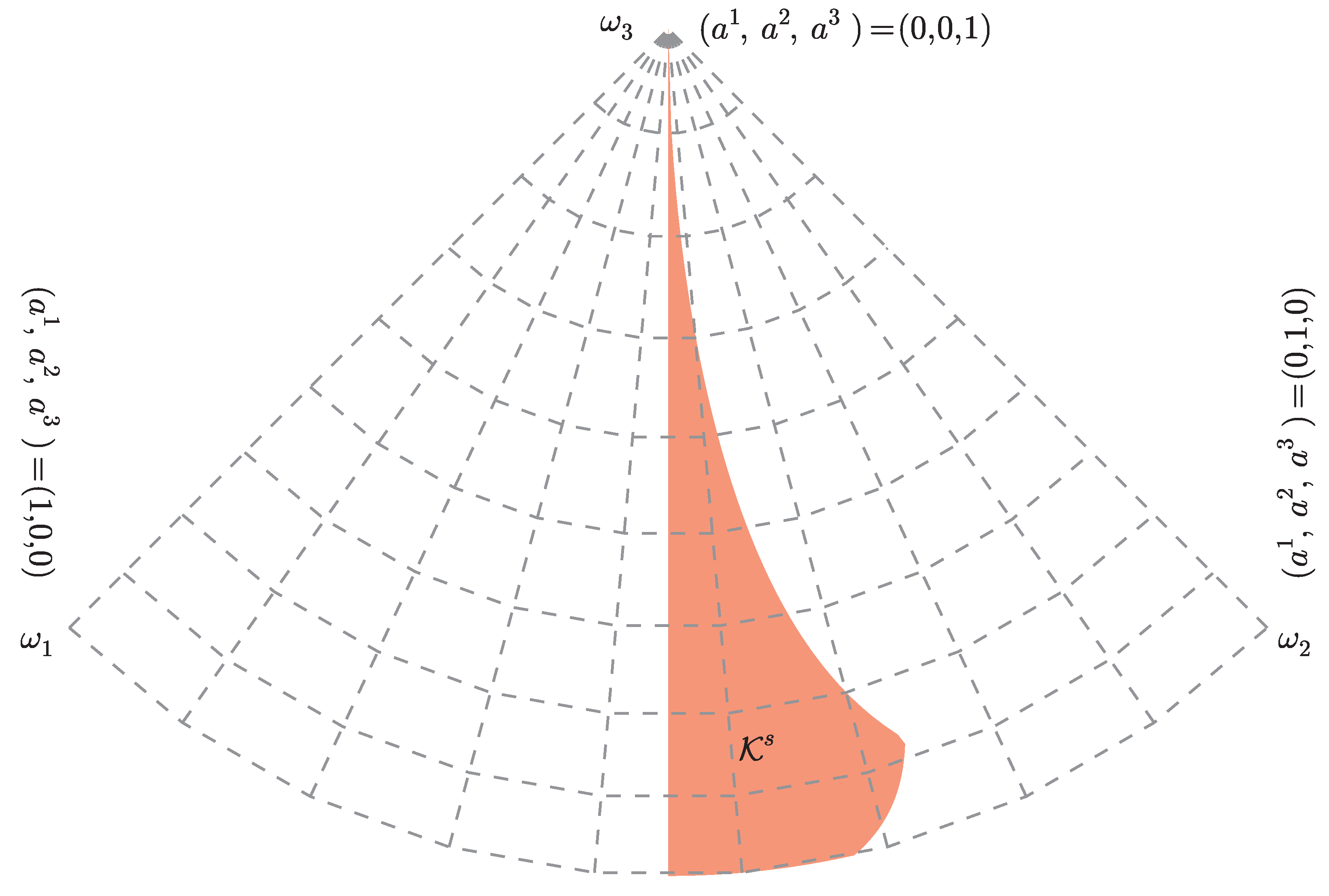
The subspace ${\mathcal{K}}^s$ satisfying (66) is a full-dimensional subcone of the Kähler cone $\mathcal{K}$ defined in (7). It is a cone because the inequalities are homogeneous. In other words, only the angular part of the Kähler moduli are constrained, but not the overall volume. Hence, it is best displayed as a two-dimensional “star map” as seen by an observer at the origin. This is shown in Figure 1. For Kähler moduli restricted to this subcone, the four-dimensional low energy theory in the observable sector is $N=1$ supersymmetric.

• Poly-Stability of the Hidden Sector Vector Bundle

To preserve $N=1$ supersymmmetry in four-dimensions, the hidden sector vector bundle, since it is generically a Whitney sum, must be poly-stable. That is, each factor of the Whitney sum must be slope-stable and, in addition, all factors in the sum must have the same slope. In order to make this more concrete, we now present three non-trivial examples to illustrate the property of poly-stability. As a first example, let us choose

• $V^{\left(2\right)}={\mathcal{V}}_N$:
  In this case, since for a single vector bundle slope-stability implies poly-stability, one need only check that ${\mathcal{V}}_N$ is slope-stable. For example, one could choose ${\mathcal{V}}_N$ to be identical to the $SU\left(4\right)$ bundle in the observable sector, $V^{\left(1\right)}$, presented above. Note that, since we are restricting all hidden sector non-Abelian bundles to have structure group $SU\left(N\right)$, it follows that $\mu \left({\mathcal{V}}_N\right)$ must vanish. As with the observable sector bundle $SU\left(4\right)$ bundle, stability of a generic non-Abelian vector bundle will only occur within a specific region of Kähler moduli space.
• $V^{\left(2\right)}=L$:
  In this case, one need only check that the line bundle L is slope-stable, which will imply poly-stability. Fortunately, every line bundle is trivially slope-stable, so any line bundle can be used. It is important to note that the slope of a line bundle which appears as a lone factor in the Whitney sum has–a priori–no further constraints. Using (65), (26) and (4), it follows that the slope of an arbitrary line bundle specified by $L={\mathcal{O}}_X({\ell }^1,{\ell }^2,{\ell }^3)$ is given by

  $$\begin{array}{c}\hfill \mu \left(L\right)=d_{ijk}{\ell }^i{a}^j{a}^k=\frac{1}{3}\left(a^2(a^2+6a^3){\ell }^1+{(a^1)}^2{\ell }^2+6a^1{a}^3{\ell }^2+2a^1{a}^2(2{\ell }^1+{\ell }^2+6{\ell }^3)\right).\end{array}$$

  (67)

  That is, its value is a highly specific function of the Kähler moduli.
• $V^{\left(2\right)}={\mathcal{V}}_N\oplus L:$
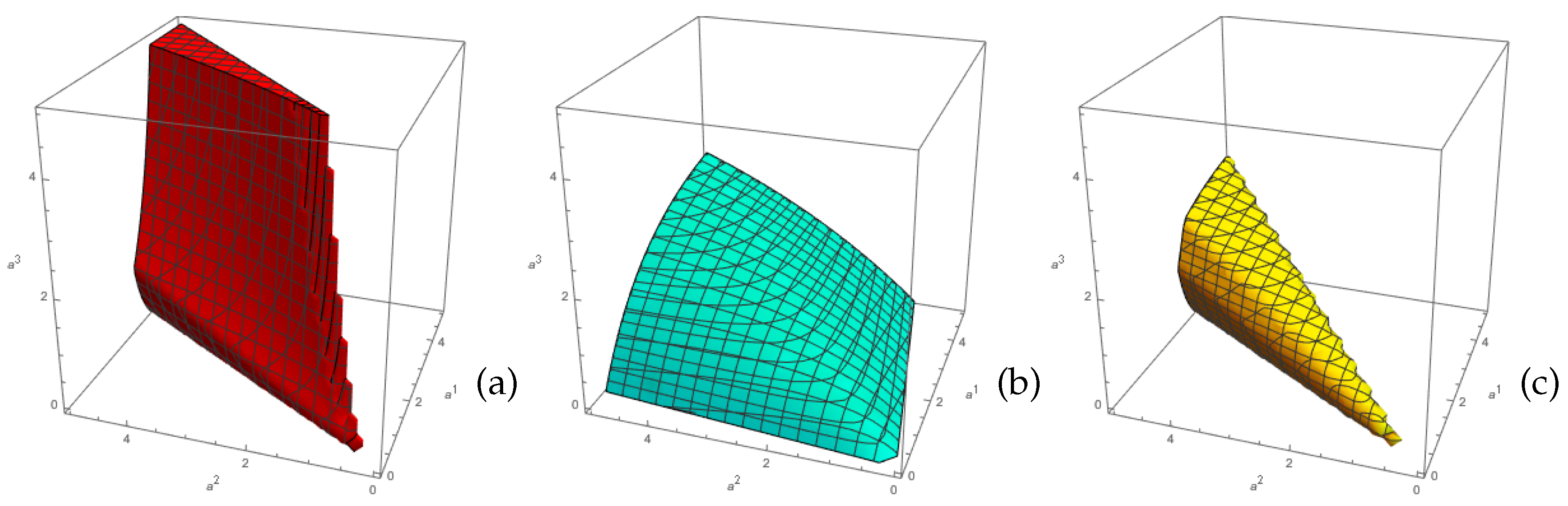
  As specified above, the non-Abelian vector bundle ${\mathcal{V}}_N$ must be slope-stable in a region of Kähler moduli space. Furthermore, since we are restricting the structure group in our discussion to be $SU\left(N\right)$, it follows that $\mu ({\mathcal{V}}_N)=0$. As we just indicated, any line bundle L will be slope-stable everywhere in Kähler moduli space. However, the full Whitney sum $V^{\left(2\right)}={\mathcal{V}}_N\oplus L$ will be poly-stable–and, hence, preserve $N=1$ supersymmetry–if and only if $\mu \left(L\right)=\mu ({\mathcal{V}}_N)=0$. That is, because of the existence of a non-Abelian $SU\left(N\right)$ factor, the line bundle L now has the additional constraint that its slope vanish identically. It is clear from (67) that this will be the case only in a restricted region of Kähler moduli space. It follows that the full Whitney sum $V^{\left(2\right)}={\mathcal{V}}_N\oplus L$ will only be a viable hidden sector bundle if the region of stability of ${\mathcal{V}}_N$ has a non-vanishing intersection with the region where the slope of L vanishes. This is a very non-trivial requirement. To give a concrete example, let us choose ${\mathcal{V}}_N=V^{\left(1\right)}$, where $V^{\left(1\right)}$ is the $SU\left(4\right)$ observable sector bundle specified above. Recall that the region of slope-stability of this bundle in Kähler moduli space is delineated by the inequalities in (66) and shown in Figure 1. Plotted in 3-dimensions, this region of slope-stability over a limited region of Kähler moduli space is shown in Figure 2a. Furthermore, let us specify that $L={\mathcal{O}}_X(1,2,-3)$. Note that L satisfies condition (23), as it must. It follows from (67) that the region of moduli space in which $\mu \left(L\right)=0$ is given by the equation

  $$\frac{2}{3}{(a^1)}^2-4a^1{a}^2+\frac{1}{3}{(a^2)}^2+4a^1{a}^3+\frac{3}{2}{a}^2{a}^3=0.$$

  (68)

  Plotted over a limited region of Kähler moduli space in 3-dimensions, the region where $\mu \left(L\right)=0$ is shown in Figure 2b. Figure 2c then shows that these two regions have a substantial overlap in Kähler moduli space. Furthermore, since ${\mathcal{V}}_N$ was chosen to be $V^{\left(1\right)}$, it follows that Figure 2c also represents the overlap with the stability region of the observable sector vector bundle. We conclude that the specific choice of $V^{\left(2\right)}=V^{\left(1\right)}\oplus {\mathcal{O}}_X(1,2,-3)$ is a suitable choice for a poly-stable hidden sector vector bundle.

These three examples give the rules for constructing specific poly-stable vector bundles. They can easily be generalized to construct generic poly-stable Whitney sum hidden sector vector bundles.

3.2. The ${\kappa }_{11}^{4/3}$ Lagrangian

The terms in the BPS double domain wall solution proportional to ${ϵ}_S^{\prime }$ lead to order ${\kappa }_{11}^{4/3}$ additions to the $d=4$ Lagrangian. These have several effects. The simplest is that the five-brane location moduli now contribute to the definition of the dilaton, which becomes

$$\mathrm{Re}S=V+{ϵ}_S^{\prime }\sum _{n=1}^N{\beta }_i^{\left(n\right)}{t}^i{z}_n^2.$$

(69)

More profoundly, these ${\kappa }_{11}^{4/3}$ terms lead to, first, additions to the Fayet-Iliopoulos (FI) term associated with any anomalous $U\left(1\right)$ factor in the low energy gauge group and, second, threshold corrections to the gauge coupling parameters. Let us analyze these in turn.

3.2.1. Corrections to a Fayet-Iliopoulos Term

In the heterotic standard model vacuum, the observable sector vector bundle $V^{\left(1\right)}$ has structure group $SU\left(4\right)$. Hence, it does not lead to an anomalous $U\left(1\right)$ gauge factor in the observable sector of the low energy theory. However, the hidden sector bundle $V^{\left(2\right)}$ introduced above, in addition to a possible non-Abelian bundle ${\mathcal{V}}_N$, consists of a sum of line bundles with the additional structure group $U{\left(1\right)}^R$. Each $U\left(1\right)$ factor leads to an anomalous $U\left(1\right)$ gauge group in the four-dimensional effective field theory and, hence, an associated D-term. Let $L_r$ be any one of the irreducible line bundles of $V^{\left(2\right)}$. The string one-loop corrected Fayet-Iliopoulos (FI) term for $L_r$ was computed in [47] within the context of the weakly coupled heterotic string. Comparing various results in the literature, it is straightforward to show that strong coupling results to order ${\kappa }_{11}^{4/3}$ can be obtained from string one-loop weak coupling expressions if one replaces

$$g_s^2{\ell }_s^4⟶{ϵ}_S^{\prime }\frac{\widehat{R}}{V^{1/3}}{v}^{2/3}$$

(70)

in the weak coupling formulas, where $g_s$ and $l_s=2\pi \sqrt{{\alpha }^{\prime }}$ are the weak coupling parameter and string length respectively and ${ϵ}_S^{\prime }$ is defined in (47). Using (70), we find that the expression for the FI term associated with $L_r$ in strongly coupled heterotic M-theory to order ${\kappa }_{11}^{4/3}$ is given by

$$F{I}_r=-\frac{{\pi }^2}{v^{1/3}V}\left(\mu \left(L_r\right)+{ϵ}_S^{\prime }\frac{\widehat{R}}{V^{1/3}}{\int }_X{c}_1\left(L_r\right)\wedge \left(J^{(N+1)}+\sum _{n=1}^N{z}_n^2{J}^{\left(n\right)}\right)\right),$$

(71)

where $\mu \left(L_r\right)$ is given in (65). Inserting (34), (6), (32) and, following the conventions of [47,50], redefining the five-brane moduli to be

$${\lambda }_n=z_n-\frac{1}{2},{\lambda }_n\in \left[-\frac{1}{2},\frac{1}{2}\right],$$

(72)

we find that

$$\begin{array}{c}F{I}_r=-\frac{{\pi }^2}{v^{1/3}V}(\mu \left(L_r\right)-{ϵ}_S^{\prime }\frac{\widehat{R}}{V^{1/3}}\hfill \\ \hspace{1em}\hspace{1em}\hspace{1em}\hspace{1em}{\int }_X{c}_1\left(L_r\right)\wedge \left(-c_2\left({\mathcal{V}}_N\right)+\sum _{s=1}^R{a}_s{c}_1\left(L_s\right)\wedge c_1\left(L_s\right)+\frac{1}{2}{c}_2\left(TX\right)-\sum _{n=1}^N{(\frac{1}{2}+{\lambda }_n)}^2{W}^{\left(n\right)}\right)),\hfill \end{array}$$

(73)

where $a_s$ is given in (29). The first term on the right-hand side, that is, the slope of $L_r$ defined in (65), is the order ${\kappa }_{11}^{2/3}$ result. The remaining terms are the ${\kappa }_{11}^{4/3}$ M-theory corrections first presented in [53]. Please note that the dimensionless parameter ${ϵ}_S^{\prime }\frac{\widehat{R}}{V^{1/3}}$ of the ${\kappa }_{11}^{4/3}$ term is identical to the expansion coefficient of the linearized solution—when expressed in term of the $a^i$ moduli—discussed in Section 2.2. See, for example, (54). Finally, recalling definition (65) of the slope, using (3), (4), (8), (26), (39) and noting from (5) that

$$\frac{1}{v^{1/3}}{\int }_X\frac{1}{2}{c}_2\left(TX\right)\wedge {\omega }_i={(2,2,0)}_i,i=1,2,3,$$

(74)

it follows that for each $L_r$ the associated Fayet-Iliopoulos factor $F{I}_r$ in (73) can be written as

$$\begin{array}{c}F{I}_r=-\frac{{\pi }^2}{v^{1/3}V}(d_{ijk}{\ell }_r^i{a}^j{a}^k-{ϵ}_S^{\prime }\frac{\widehat{R}}{V^{1/3}}\hfill \\ \hspace{1em}\hspace{1em}\hspace{1em}\hspace{1em}\hspace{1em}\hspace{1em}\hspace{1em}\hspace{1em}\hspace{1em}(-d_{ijk}{\ell }_r^i{c}_N^{jk}+d_{ijk}{\ell }_r^i\sum _{s=1}^R{a}_s{\ell }_s^j{\ell }_s^k+{\ell }_r^i{(2,2,0)|}_i-\sum _{n=1}^N{(\frac{1}{2}+{\lambda }_n)}^2{\ell }_r^i{W}_i^{\left(n\right)}))\hfill \end{array}$$

(75)

where

$$V=\frac{1}{6}{d}_{ijk}{a}^i{a}^j{a}^k.$$

(76)

As discussed in [53], the general form of each D-term in the low energy four-dimensional theory is the sum of (1) the moduli dependent FI parameter (75) and (2) terms quadratic in the four-dimensional scalar fields charged under the associated $U\left(1\right)$ gauge symmetry weighted by their specific charge. For each line bundle $L_r$, $r=1,\dots ,R$ on the Calabi-Yau threefold, there is an anomalous $U{\left(1\right)}_r$ symmetry in the four-dimensional low energy theory on the hidden sector. The associated D-term is given by

$$D_r=F{I}_r+\sum _{\alpha }{q}_{\alpha }^r{|{\varphi }_{\alpha }^r|}^2,$$

(77)

where the ${\varphi }_{\alpha }^r$ denote scalar fields of mass dimension one with charge $q_{\alpha }^r$ under this $U{\left(1\right)}_r$ Abelian gauge symmetry. Note from (75) that $F{I}_r$ has mass dimension two–consistent with expression (77). As is well-known, a necessary condition for a static vacuum state of the theory to be $N=1$ supersymmetric is that the D term associated with each line bundle $L_r$ must identically vanish. Generically, this will be the case if

$$\sum _{\alpha }{q}_{\alpha }^r{\left|\langle {\varphi }_{\alpha }^r\rangle \right|}^2=-F{I}_r.$$

(78)

These ${\varphi }_{\alpha }^r$ scalars break into two distinct types—(1) those that transform only under the Abelian group $U{\left(1\right)}_r$ and (2) those which, in addition, transform non-trivially under the non-Abelian gauge factor of the hidden sector low energy theory. This second type of scalar field will also appear in the D-term associated with the non-Abelian group–which cannot contain a FI term. Hence, the demand that the vacuum be supersymmetric generically sets their vacuum expectation values to zero. It follow that one can, henceforth, ignore such fields and restrict the scalars in (78) to those that transform under the Abelian $U{\left(1\right)}_r$ symmetry only.

In the weakly coupled heterotic case discussed in [46], it was assumed, for simplicity, that the vacuum expectation values $\langle {\varphi }_{\alpha }^r\rangle$ all vanish, even for the scalars not transforming under the low energy non-Abelian gauge factor. In that case, each $D_r$ will vanish if and only if $F{I}_r=0$. This restriction puts very strong constraints on the choice of the hidden sector vector bundle. Be that as it may, the assumption that all $\langle {\varphi }_{\alpha }^r\rangle$ vanish and that $F{I}_r=0$ remains a valid constraint for strongly coupled vacua. However, in the strongly coupled case we are now considering, an alternative set of constraints can be also be adopted. That is, one can assume that the scalar fields that only transform under the low energy $U{\left(1\right)}_r$ groups are, in general, non-vanishing and that each $D_r$ is set to zero by the associated vacuum expectation values $\langle {\varphi }_{\alpha }^r\rangle$ becoming non-zero. For this to be the case, it is essential to specify the hidden sector vector bundle and to compute the pure $U{\left(1\right)}_r$ low energy scalar fields ${\varphi }_{\alpha }^r$ and their associated charges $q_{\alpha }^r$. This is essential because, should the $U{\left(1\right)}_r$ charge be positive, then the associated $D_r$ term can vanish if and only if $F{I}_r<0$. On the other hand, if the associated charge is negative, then $D_r$ can vanish if and only if $F{I}_r>0$. That is, the condition one needs to impose on the Fayet-Iliopoulos terms will depend on the sign of the charge of the scalar spectrum.

3.2.2. Gauge Threshold Corrections

The gauge couplings of the non-anomalous components of the $d=4$ gauge group, in both the observable and hidden sectors, have been computed to order ${\kappa }_{11}^{4/3}$ in [53]. Including five-branes in the bulk space, these are given by

$$\frac{4\pi }{{(g^{\left(1\right)})}^2}=V+{ϵ}_S^{\prime }\frac{\widehat{R}}{2V^{1/3}}\sum _{n=0}^{N+1}{(1-z_n)}^2{a}^i{\beta }_i^{\left(n\right)}$$

(79)

and

$$\frac{4\pi }{{(g^{\left(2\right)})}^2}=V+{ϵ}_S^{\prime }\frac{\widehat{R}}{2V^{1/3}}\sum _{n=1}^{N+1}{z}_n^2{a}^i{\beta }_i^{\left(n\right)}$$

(80)

respectively. Using (34), (41) and (6), (10), (27), (28), (72), it follows that

$$\begin{array}{cc}\hfill \frac{4\pi }{{(g^{\left(1\right)})}^2}=& \frac{1}{6v}{\int }_X\omega \wedge \omega \wedge \omega -{ϵ}_S^{\prime }\frac{\widehat{R}}{2V^{1/3}}\frac{1}{v^{1/3}}\hfill \\ & \times {\int }_X\omega \wedge \left(-c_2(V^{\left(1\right)})+\frac{1}{2}{c}_2\left(TX\right)-\sum _{n=1}^N{(\frac{1}{2}-{\lambda }_n)}^2{W}^{\left(n\right)}\right)\hfill \end{array}$$

(81)

and

$$\begin{array}{cc}\hfill \frac{4\pi }{{(g^{\left(2\right)})}^2}=& \frac{1}{6v}{\int }_X\omega \wedge \omega \wedge \omega -{ϵ}_S^{\prime }\frac{\widehat{R}}{2V^{1/3}}\frac{1}{v^{1/3}}\hfill \\ & \times {\int }_X\omega \wedge \left(-c_2({\mathcal{V}}_N)+\sum _{r=1}^R{a}_r{c}_1(L_r)\wedge c_1\left(L_r\right)+\frac{1}{2}{c}_2\left(TX\right)-\sum _{n=1}^N{(\frac{1}{2}+{\lambda }_n)}^2{W}^{\left(n\right)}\right)\hfill \end{array}$$

(82)

where $a_r$ is given in (29). The first term on the right-hand side, that is, the volume V defined in (10), is the order ${\kappa }_{11}^{2/3}$ result. The remaining terms are the ${\kappa }_{11}^{4/3}$ M-theory corrections first presented in [53].

Clearly, consistency of the $d=4$ effective theory requires both ${(g^{\left(1\right)})}^2$ and ${(g^{\left(2\right)})}^2$ to be positive. It follows that the moduli of the four-dimensional theory are constrained to satisfy

$$\begin{array}{c}\hfill \frac{1}{v}{\int }_X\omega \wedge \omega \wedge \omega -3{ϵ}_S^{\prime }\frac{\widehat{R}}{V^{1/3}}\frac{1}{v^{1/3}}{\int }_X\omega \wedge \left(-c_2(V^{\left(1\right)})+\frac{1}{2}{c}_2\left(TX\right)-\sum _{n=1}^N{(\frac{1}{2}-{\lambda }_n)}^2{W}^{\left(n\right)}\right)>0\end{array}$$

(83)

and

$$\begin{array}{c}\hfill \frac{1}{v}{\int }_X\omega \wedge \omega \wedge \omega -3{ϵ}_S^{\prime }\frac{\widehat{R}}{V^{1/3}}\frac{1}{v^{1/3}}{\int }_X\omega \wedge (-c_2({\mathcal{V}}_N)+\sum _{r=1}^R{a}_r{c}_1(L_r)\wedge c_1(L_r)\hspace{1em}\hspace{1em}\hspace{1em}\hspace{1em}\hspace{1em}\hspace{1em}\hspace{1em}\\ \hfill +\frac{1}{2}{c}_2\left(TX\right)-\sum _{n=1}^N{(\frac{1}{2}+{\lambda }_n)}^2{W}^{\left(n\right)})>0.\end{array}$$

(84)

Please note that the dimensionless parameter ${ϵ}_S^{\prime }\frac{\widehat{R}}{V^{1/3}}$ of the ${\kappa }_{11}^{4/3}$ term is identical to the expansion coefficient of both the FI condition (75) and the linearized solution discussed in Section 2.2. As in the previous subsections, one can use (3), (4), (5), (8), (15), (19), (26) and (39) to rewrite these expressions as

$$\begin{array}{c}\hfill d_{ijk}{a}^i{a}^j{a}^k-3{ϵ}_S^{\prime }\frac{\widehat{R}}{V^{1/3}}(-(\frac{8}{3}{a}^1+\frac{5}{3}{a}^2+4a^3)+\hspace{1em}\hspace{1em}\\ \hfill +2(a^1+a^2)-\sum _{n=1}^N{(\frac{1}{2}-{\lambda }_n)}^2{a}^i{W}_i^{\left(n\right)})>0\end{array}$$

(85)

and

$$\begin{array}{c}\hfill d_{ijk}{a}^i{a}^j{a}^k-3{ϵ}_S^{\prime }\frac{\widehat{R}}{V^{1/3}}(-d_{ijk}{a}^i{c}_N^{jk}+d_{ijk}{a}^i\sum _{r=1}^R{a}_r{\ell }_r^j{\ell }_r^k+\hspace{1em}\hspace{1em}\\ \hfill +2(a^1+a^2)-\sum _{n=1}^N{(\frac{1}{2}+{\lambda }_n)}^2{a}^i{W}_i^{\left(n\right)})>0\end{array}$$

(86)

respectively.

Again, it is of interest to compare the ${(g^{\left(1\right)})}^2$, ${(g^{\left(2\right)})}^2>0$ conditions calculated to order ${\kappa }_{11}^{4/3}$ in strongly coupled heterotic M-theory, that is, (83) and (84), to the one-loop corrected conditions computed in the weakly coupled heterotic string [50]. Assuming the same observable and hidden sector vector bundles used in this paper, we find that the weakly coupled conditions for ${(g^{\left(1\right)})}^2$, ${(g^{\left(2\right)})}^2>0$, derived using (3.103) in [50], are identical to (83) and (84) if one again uses the replacement $g_s^2{\ell }_s^4⟶{ϵ}_S^{\prime }\frac{\widehat{R}}{V^{1/3}}{v}^{2/3}$ given in (70).

3.3. A Specific Class of Examples

The constraint equations listed above are technically rather complicated. Therefore, as we did when discussing poly-stability in Section 3.1, we now analyze the constraint equations within the context of a specific class of $N=1$ supersymmetric hidden sector vector bundles. To do this, one must specify the non-Abelian bundle ${\mathcal{V}}_N$ with structure group $SU\left(N\right)$, the number of line bundles $L_r$ and their exact embeddings into the hidden $E_8$ vector bundle. We will, henceforth, consider hidden sector bundles that may, or may not, contain a non-Abelian factor and, for simplicity, are restricted to contain at most a single line bundle

$$L={\mathcal{O}}_X({\ell }^1,{\ell }^2,{\ell }^3)$$

(87)

where

$${\ell }^1,{\ell }^2,{\ell }^3\in \mathbb{Z},({\ell }^1+{\ell }^2)\mathrm{mod}3=0.$$

(88)

In this case, there is only a single $a_r$ coefficient–which we denote simply by a. In addition, one must specify the number of five-branes in the bulk space. Again, for simplicity, we assume that there is only one five-brane in this example. It then follows from (40), (75), (85), and (86) that the constraints for this restricted class of examples are given by

$$\begin{array}{c}\hfill W_i=\left(\frac{4}{3},\frac{7}{3},-4\right){|}_i-d_{ijk}{c}_N^{jk}+a{d}_{ijk}{\ell }^j{\ell }^k\ge 0,i=1,2,3,\end{array}$$

(89)

$$\begin{array}{c}\hfill \begin{array}{cc}\hfill d_{ijk}{\ell }^i{a}^j{a}^k-{ϵ}_S^{\prime }\frac{\widehat{R}}{V^{1/3}}(-d_{ijk}{\ell }^i{c}_N^{jk}+a{d}_{ijk}{\ell }^i{\ell }^j{\ell }^k& \\ \hfill +{\ell }^i{(2,2,0)|}_i-{(\frac{1}{2}+\lambda )}^2{\ell }^i{W}_i)& \lessgtr 0,=0\hfill \end{array}\end{array}$$

(90)

$$\begin{array}{c}\hfill \begin{array}{cc}\hfill d_{ijk}{a}^i{a}^j{a}^k-3{ϵ}_S^{\prime }\frac{\widehat{R}}{V^{1/3}}(-\left(\frac{8}{3}{a}^1+\frac{5}{3}{a}^2+4a^3\right)& \\ \hfill +2(a^1+a^2)-{\left(\frac{1}{2}-\lambda \right)}^2{a}^i{W}_i)& >0\hfill \end{array}\end{array}$$

(91)

$$\begin{array}{c}\hfill \begin{array}{cc}\hfill d_{ijk}{a}^i{a}^j{a}^k-3{ϵ}_S^{\prime }\frac{\widehat{R}}{V^{1/3}}(-d_{ijk}{a}^i{c}_N^{jk}+a{d}_{ijk}{a}^i{\ell }^j{\ell }^k& \\ \hfill +2(a^1+a^2)-{(\frac{1}{2}+\lambda )}^2{a}^i{W}_i)& >0\hfill \end{array}\end{array}$$

(92)

where $\widehat{R}$ is an independent modulus and V satisfies relation (76). Note that the expression on the left-hand side of the (90) is a) $>0$ or $<0$ if one assumes that some $\langle {\varphi }_{\alpha }\rangle \ne 0$ and that the associated scalar charge $q_{\alpha }$ is positive or negative respectively or b) $=0$ if, alternatively, one assumes that all $\langle {\varphi }_{\alpha }\rangle =0$.

To proceed, one must specify the the coefficient a, as well as the coefficients $c_N^{jk}$ of the second Chern class of ${\mathcal{V}}_N$. We begin with the coefficient a. Recall from (29) that

$$a=\frac{1}{4·30}{tr}_{E_8}{Q}^2,$$

(93)

where Q is the generator of the $U\left(1\right)$ structure group of the line bundle. Hence, the value of coefficient a will depend entirely on the explicit embedding of this $U\left(1\right)$ into the $\underline{\mathbf{248}}$ representation of the hidden sector $E_8$. This will be specified as follows. Choose the structure group $SU\left(N\right)$ of ${\mathcal{V}}_N$ and embed

$$SU\left(N\right)\times U\left(1\right)\subset SU(N+1).$$

(94)

The structure group of the line bundle L is identified with the specific $U\left(1\right)$ generator in $SU(N+1)$ which commutes with the generators of the chosen $SU\left(N\right)$. In the fundamental representation of $SU(N+1)$, the generator of $U\left(1\right)$ can then be written as

$$\mathrm{diag}(\underset{N}{\underbrace{1,\dots ,1}},-N).$$

(95)

This specifies the exact embedding of $U\left(1\right)$ into $SU(N+1)$. Now choose $SU(N+1)$ to be a factor of a maximal subgroup of $E_8$. The decomposition of the $\underline{\mathbf{248}}$ of $E_8$ with respect to this maximal subgroup, together with (95), then determines the generator Q.

This is most easily explained by giving a simple explicit example. Let us assume there is no non-Abelian bundle–only a single line bundle. That is,

$$V^{\left(2\right)}=L.$$

(96)

The explicit embedding of L into $E_8$ is chosen as follows. First, recall that

$$SU\left(2\right)\times E_7\subset E_8$$

(97)

is a maximal subgroup. With respect to $SU\left(2\right)\times E_7$, the $\underline{\mathbf{248}}$ representation of $E_8$ decomposes as

$$\underline{\mathbf{248}}⟶(\underline{\mathbf{1}},\underline{\mathbf{133}})\oplus (\underline{\mathbf{2}},\underline{\mathbf{56}})\oplus (\underline{\mathbf{3}},\underline{\mathbf{1}}).$$

(98)

Now choose the generator of the $U\left(1\right)$ structure group in the fundamental representation of $SU\left(2\right)$ to be $(1,-1)$. It follows that under $SU\left(2\right)\to U\left(1\right)$

$$\underline{\mathbf{2}}⟶1\oplus -1$$

(99)

and, hence, under $U\left(1\right)\times E_7$

$$\underline{\mathbf{248}}⟶(0,\underline{\mathbf{133}})\oplus \left((1,\underline{\mathbf{56}})\oplus (-1,\underline{\mathbf{56}})\right)\oplus \left((2,\underline{\mathbf{1}})\oplus (0,\underline{\mathbf{1}})\oplus (-2,\underline{\mathbf{1}})\right).$$

(100)

The generator Q of this embedding of the line bundle can be read off from expression (100). Inserting this into (93), we find that

$$a=1.$$

(101)

For the choice of a non-Abelian bundle ${\mathcal{V}}_N$ with structure group $SU\left(N\right)$, similar calculations give

$$N=2\Rightarrow a=3,N=3\Rightarrow a=6,N=4\Rightarrow a=10,N=5\Rightarrow a=15$$

(102)

As discussed previously, one may or may not include a non-Abelian factor in the hidden sector vector bundle. If a non-Abelian factor ${\mathcal{V}}_N$ is to be included, one must specify it exactly. Generically, there are many possibilities for such a bundle. As an explicit example, let us choose this to be precisely the same $SU\left(4\right)$ bundle as in the observable sector described in Section 2.1.2. Doing this greatly simplifies the analysis since this ${\mathcal{V}}_4$ bundle is slope-stable with vanishing slope in the same region of Kähler moduli space as the observable sector bundle $V^{\left(1\right)}$—that is, when the inequalities (66) are satisfied. Since $N=4$, it follows from (102) that coefficient

$$a=10$$

(103)

and, since ${\mathcal{V}}_4$ is identical to $V^{\left(1\right)}$, it follows from (15) that

$$c_2({\mathcal{V}}_4)=\frac{1}{v^{2/3}}\left({\omega }_1\wedge {\omega }_1+4{\omega }_2\wedge {\omega }_2+4{\omega }_1\wedge {\omega }_2\right).$$

(104)

Hence, from (19) the only non-vanishing $c_N^{jk}$ coefficients are

$$c_4^{11}=1,c_4^{22}=4,c_4^{12}=c_4^{21}=2.$$

(105)

Inserting these coefficients, along with a = 10, into (89), (90), (91), (92) give the appropriate constraint equations for this class of vacua. As discussed above, if one assumes the VEVs of all scalar fields vanish, then the left-hand side of (90) must be zero. However, if not all $\langle {\varphi }_{\alpha }\rangle$ vanish, then to determine whether the left-hand side of the FI inequality (90) is $>0$ or $<0$ depends on the sign of the charge of the associated low energy $U\left(1\right)$ charged scalars. Since the charge can be different for different choices of the hidden sector bundle, this can only be determined within the context of an explicit example. This will be presented elsewhere.

Of course, these constraints have to be solved simultaneously with the condition (66) for the slope-stability of both the observable and hidden sector non-Abelian vector bundles; that is

$$\begin{array}{c}\left(a^1<a^2\le \sqrt{\frac{5}{2}}{a}^1\mathrm{and}{a}^3<\frac{-{\left(a^1\right)}^2-3a^1{a}^2+{\left(a^2\right)}^2}{6a^1-6a^2}\right)\mathrm{or}\\ \left(\sqrt{\frac{5}{2}}{a}^1<a^2<2a^1\mathrm{and}\frac{2{\left(a^2\right)}^2-5{\left(a^1\right)}^2}{30a^1-12a^2}<a^3<\frac{-{\left(a^1\right)}^2-3a^1{a}^2+{\left(a^2\right)}^2}{6a^1-6a^2}\right)\end{array}$$

(106)

Finally, it is essential to implement Equations (57) and (58) for the validity of the linear approximation. These equations depend sensitively on the sign of each component of ${\beta }_i^{\left(0\right)}$, the value of ${\beta }_i^{\left(1\right)}=W_i$ and the five-brane location $z_1$. For the specific class of models presented in this section, (57) and (58) become

$$2{ϵ}_S^{\prime }\frac{\widehat{R}}{V^{1/3}}\left|{\beta }_i^{\left(0\right)}\left(z-\frac{1}{2}\right)-\frac{1}{2}{W}_i{(\frac{1}{2}-\lambda )}^2\right|\ll \left|d_{ijk}{a}^j{a}^k\right|,z\in [0,\lambda +\frac{1}{2}]$$

(107)

and

$$2{ϵ}_S^{\prime }\frac{\widehat{R}}{V^{1/3}}\left|({\beta }_i^{\left(0\right)}+W_i)\left(z-\frac{1}{2}\right)-\frac{1}{2}{W}_i{(\frac{1}{2}+\lambda )}^2\right|\ll \left|d_{ijk}{a}^j{a}^k\right|,z\in [\lambda +\frac{1}{2},1].$$

(108)

References

- Gross, D.J.; Harvey, J.A.; Martinec, E.J.; Rohm, R. Heterotic String Theory. 1. The Free Heterotic String. Nucl. Phys. B 1985, 256, 253–284. [Google Scholar] [CrossRef]
- Gross, D.J.; Harvey, J.A.; Martinec, E.J.; Rohm, R. Heterotic String Theory. 2. The Interacting Heterotic String. Nucl. Phys. B 1986, 267, 75–124. [Google Scholar] [CrossRef]
- Witten, E. Strong coupling expansion of Calabi-Yau compactification. Nucl. Phys. B 1996, 471, 135–158. [Google Scholar] [CrossRef] [Green Version]
- Horava, P.; Witten, E. Heterotic and type I string dynamics from eleven dimensions. Nucl. Phys. B 1996, 460, 506–524. [Google Scholar] [CrossRef]
- Horava, P.; Witten, E. Eleven-dimensional supergravity on a manifold with boundary. Nucl. Phys. B 1996, 475, 94–114. [Google Scholar] [CrossRef] [Green Version]
- Greene, B.R.; Kirklin, K.H.; Miron, P.J.; Ross, G.G. A Superstring Inspired Standard Model. Phys. Lett. B 1986, 180, 69–76. [Google Scholar] [CrossRef]
- Greene, B.R.; Kirklin, K.H.; Miron, P.J.; Ross, G.G. A Three Generation Superstring Model. 1. Compactification and Discrete Symmetries. Nucl. Phys. 1986, B278, 667–693. [Google Scholar] [CrossRef]
- Greene, B.R.; Kirklin, K.H.; Miron, P.J.; Ross, G.G. A Three Generation Superstring Model. 2. Symmetry Breaking and the Low-Energy Theory. Nucl. Phys. B 1987, 292, 606–652. [Google Scholar] [CrossRef]
- Matsuoka, T.; Suematsu, D. Realistic Models From The E8 × Superstring Theory. Prog. Theor. Phys. 1986, 76, 886–900. [Google Scholar] [CrossRef]
- Greene, B.R.; Kirklin, K.H.; Miron, P.J.; Ross, G.G. 273 Yukawa Couplings For a Three Generation Superstring Model. Phys. Lett. B 1987, 192, 111. [Google Scholar] [CrossRef]
- Anderson, L.B.; Gray, J.; Lukas, A.; Ovrut, B. Stabilizing All Geometric Moduli in Heterotic Calabi-Yau Vacua. Phys. Rev. D 2011, 83, 106011. [Google Scholar] [CrossRef]
- Braun, V.; He, Y.H.; Ovrut, B.A.; Pantev, T. The Exact MSSM spectrum from string theory. J. High Energy Phys. 2006, 2006, 043. [Google Scholar] [CrossRef]
- Braun, V.; Ovrut, B.A.; Pantev, T.; Reinbacher, R. Elliptic Calabi-Yau threefolds with Z(3) × Z(3) Wilson lines. J. High Energy Phys. 2004, 2004, 062. [Google Scholar] [CrossRef]
- Braun, V.; He, Y.H.; Ovrut, B.A.; Pantev, T. Vector Bundle Extensions, Sheaf Cohomology, and the Heterotic Standard Model. Adv. Theor. Math. Phys. 2006, 10, 525–529. [Google Scholar] [CrossRef]
- Braun, V.; He, Y.H.; Ovrut, B.A. Stability of the minimal heterotic standard model bundle. J. High Energy Phys. 2006, 2006, 032. [Google Scholar] [CrossRef]
- Braun, V.; He, Y.H.; Ovrut, B.A. Yukawa couplings in heterotic standard models. J. High Energy Phys. 2006, 2006, 019. [Google Scholar] [CrossRef]
- Barger, V.; Fileviez Perez, P.; Spinner, S. Minimal gauged U(1)(B-L) model with spontaneous R-parity violation. Phys. Rev. Lett. 2009, 102, 181802. [Google Scholar] [CrossRef]
- Fileviez Perez, P.; Spinner, S. Spontaneous R-Parity Breaking in SUSY Models. Phys. Rev. D 2009, 80, 015004. [Google Scholar] [CrossRef]
- Ambroso, M.; Ovrut, B. The B-L/Electroweak Hierarchy in Heterotic String and M-Theory. J. High Energy Phys. 2009, 2009, 011. [Google Scholar] [CrossRef]
- Ambroso, M.; Ovrut, B.A. The B-L/Electroweak Hierarchy in Smooth Heterotic Compactifications. Int. J. Mod. Phys. A 2010, 25, 2631–2677. [Google Scholar] [CrossRef]
- Ambroso, M.; Ovrut, B.A. The Mass Spectra, Hierarchy and Cosmology of B-L MSSM Heterotic Compactifications. Int. J. Mod. Phys. A 2011, 26, 1569–1627. [Google Scholar] [CrossRef]
- Ovrut, B.A.; Purves, A.; Spinner, S. Wilson Lines and a Canonical Basis of SU(4) Heterotic Standard Models. J. High Energy Phys. 2012, 2012, 026. [Google Scholar] [CrossRef]
- Ovrut, B.A.; Purves, A.; Spinner, S. The minimal SUSY B − L model: From the unification scale to the LHC. J. High Energy Phys. 2015, 2015, 182. [Google Scholar] [CrossRef]
- Fileviez Perez, P.; Spinner, S. TeV Scale Spontaneous R-Parity Violation. AIP Conf. Proc. 2010, 1200, 529–532. [Google Scholar] [CrossRef]
- Fileviez Perez, P.; Spinner, S. The Minimal Theory for R-parity Violation at the LHC. J. High Energy Phys. 2012, 1204, 118. [Google Scholar] [CrossRef]
- Brelidze, T.; Ovrut, B.A. B-L Cosmic Strings in Heterotic Standard Models. J. High Energy Phys. 2010, 2010, 077. [Google Scholar] [CrossRef]
- Battarra, L.; Koehn, M.; Lehners, J.L.; Ovrut, B.A. Cosmological Perturbations Through a Non-Singular Ghost-Condensate/Galileon Bounce. J. Cosmol. Astropart. Phys. 2014, 1407, 007. [Google Scholar] [CrossRef]
- Koehn, M.; Lehners, J.L.; Ovrut, B.A. Cosmological super-bounce. Phys. Rev. D 2014, 90, 025005. [Google Scholar] [CrossRef]
- Koehn, M.; Lehners, J.L.; Ovrut, B.A. Higher-Derivative Chiral Superfield Actions Coupled to N = 1 Supergravity. Phys. Rev. D 2012, 86, 085019. [Google Scholar] [CrossRef]
- Marshall, Z.; Ovrut, B.A.; Purves, A.; Spinner, S. Spontaneous R-Parity Breaking, Stop LSP Decays and the Neutrino Mass Hierarchy. Phys. Lett. B 2014, 732, 325–329. [Google Scholar] [CrossRef]
- Marshall, Z.; Ovrut, B.A.; Purves, A.; Spinner, S. LSP Squark Decays at the LHC and the Neutrino Mass Hierarchy. Phys. Rev. D 2014, 90, 015034. [Google Scholar] [CrossRef]
- Dumitru, S.; Ovrut, B.A.; Purves, A. The R-parity Violating Decays of Charginos and Neutralinos in the B-L MSSM. arXiv, 2018; arXiv:1810.11035. [Google Scholar]
- Dumitru, S.; Ovrut, B.A.; Purves, A. R-parity Violating Decays of Wino Chargino and Wino Neutralino LSPs and NLSPs at the LHC. arXiv, 2018; arXiv:1811.05581. [Google Scholar]
- Candelas, P.; de la Ossa, X.; He, Y.H.; Szendroi, B. Triadophilia: A Special Corner in the Landscape. Adv. Theor. Math. Phys. 2008, 12, 429–473. [Google Scholar] [CrossRef]
- Anderson, L.B.; Gray, J.; Lukas, A.; Palti, E. Two Hundred Heterotic Standard Models on Smooth Calabi-Yau Threefolds. Phys. Rev. D 2011, 84, 106005. [Google Scholar] [CrossRef]
- Anderson, L.B.; Gray, J.; Lukas, A.; Palti, E. Heterotic Line Bundle Standard Models. J. High Energy Phys. 2012, 2012, 113. [Google Scholar] [CrossRef]
- Anderson, L.B.; Gray, J.; Lukas, A.; Palti, E. Heterotic standard models from smooth Calabi-Yau three-folds. PoS 2011, CORFU2011, 096. [Google Scholar]
- Kachru, S.; Kallosh, R.; Linde, A.D.; Trivedi, S.P. De Sitter vacua in string theory. Phys. Rev. D 2003, 68, 046005. [Google Scholar] [CrossRef]
- Gray, J.; Lukas, A.; Ovrut, B. Perturbative anti-brane potentials in heterotic M-theory. Phys. Rev. D 2007, 76, 066007. [Google Scholar] [CrossRef]
- Gray, J.; Lukas, A.; Ovrut, B. Flux, gaugino condensation and anti-branes in heterotic M-theory. Phys. Rev. D 2007, 76, 126012. [Google Scholar] [CrossRef]
- Braun, V.; Ovrut, B.A. Stabilizing moduli with a positive cosmological constant in heterotic M-theory. J. High Energy Phys. 2006, 2006, 035. [Google Scholar] [CrossRef]
- Bogomolov, F.A. Holomorphic tensors and vector bundles on projective manifolds. Izvestiya Rossiiskoi Akademii Nauk Seriya Matematicheskaya 1978, 42, 1227–1287, 1439. [Google Scholar]
- Douglas, M.R.; Reinbacher, R.; Yau, S.T. Branes, bundles and attractors: Bogomolov and beyond. arXiv, 2006; arXiv:math/0604597. [Google Scholar]
- Andreas, B.; Curio, G. Spectral Bundles and the DRY-Conjecture. J. Geom. Phys. 2012, 62, 800–803. [Google Scholar] [CrossRef]
- Andreas, B.; Curio, G. On the Existence of Stable bundles with prescribed Chern classes on Calabi-Yau threefolds. arXiv, 2011; arXiv:1104.3435. [Google Scholar]
- Braun, V.; He, Y.H.; Ovrut, B.A. Supersymmetric Hidden Sectors for Heterotic Standard Models. J. High Energy Phys. 2013, 2013, 008. [Google Scholar] [CrossRef]
- Blumenhagen, R.; Honecker, G.; Weigand, T. Loop-corrected compactifications of the heterotic string with line bundles. J. High Energy Phys. 2005, 2005, 020. [Google Scholar] [CrossRef]
- Blumenhagen, R.; Honecker, G.; Weigand, T. Non-Abelian brane worlds: The Heterotic string story. J. High Energy Phys. 2005, 2005, 086. [Google Scholar] [CrossRef]
- Blumenhagen, R.; Moster, S.; Weigand, T. Heterotic GUT and standard model vacua from simply connected Calabi-Yau manifolds. Nucl. Phys. B 2006, 751, 186–221. [Google Scholar] [CrossRef]
- Weigand, T. Compactifications of the heterotic string with unitary bundles. Fortsch. Phys. 2006, 54, 963–1077. [Google Scholar] [CrossRef] [Green Version]
- Blumenhagen, R.; Moster, S.; Reinbacher, R.; Weigand, T. Massless Spectra of Three Generation U(N) Heterotic String Vacua. J. High Energy Phys. 2007, 2007, 041. [Google Scholar] [CrossRef]
- Blumenhagen, R.; Honecker, G.; Weigand, T. Supersymmetric (non-)Abelian bundles in the Type I and SO(32) heterotic string. J. High Energy Phys. 2005, 2005, 009. [Google Scholar] [CrossRef]
- Lukas, A.; Ovrut, B.A.; Waldram, D. Nonstandard embedding and five-branes in heterotic M theory. Phys. Rev. D 1999, 59, 106005. [Google Scholar] [CrossRef]
- Donagi, R.; Ovrut, B.A.; Waldram, D. Moduli spaces of five-branes on elliptic Calabi-Yau threefolds. J. High Energy Phys. 1999, 1999, 030. [Google Scholar] [CrossRef]
- Lukas, A.; Ovrut, B.A.; Waldram, D. Five-branes and supersymmetry breaking in M theory. J. High Energy Phys. 1999, 1999, 009. [Google Scholar] [CrossRef]
- Lukas, A.; Ovrut, B.A.; Waldram, D. On the four-dimensional effective action of strongly coupled heterotic string theory. Nucl. Phys. B 1998, 532, 43–82. [Google Scholar] [CrossRef] [Green Version]
- Anderson, L.B.; Gray, J.; Lukas, A.; Ovrut, B. Stability Walls in Heterotic Theories. J. High Energy Phys. 2009, 2009, 026. [Google Scholar] [CrossRef]
- Schoen, C. On fiber products of rational elliptic surfaces with section. Math. Z. 1988, 197, 177–199. [Google Scholar] [CrossRef]
- Lukas, A.; Ovrut, B.A.; Stelle, K.; Waldram, D. Heterotic M theory in five-dimensions. Nucl. Phys. B 1999, 552, 246–290. [Google Scholar] [CrossRef]
- Donagi, R.; Lukas, A.; Ovrut, B.A.; Waldram, D. Nonperturbative vacua and particle physics in M theory. J. High Energy Phys. 1999, 1999, 018. [Google Scholar] [CrossRef]
- Lukas, A.; Ovrut, B.A.; Stelle, K.; Waldram, D. The Universe as a domain wall. Phys. Rev. D 1999, 59, 086001. [Google Scholar] [CrossRef]
- Donagi, R.; Lukas, A.; Ovrut, B.A.; Waldram, D. Holomorphic vector bundles and nonperturbative vacua in M theory. J. High Energy Phys. 1999, 1999, 034. [Google Scholar] [CrossRef]
- Uhlenbeck, K.; Yau, S.T. On the existence of hermitian-Yang-Mills connections in stable vector bundles. Commun. Pure Appl. Math. 1986, 39, S257–S293. [Google Scholar] [CrossRef]
- Donaldson, S.K. Anti self-dual Yang-Mills connections over complex algebraic surfaces and stable vector bundles. Proc. Lond. Math. Soc. 1985, 50, 1–26. [Google Scholar] [CrossRef]
- Green, M.B.; Schwarz, J.H.; Witten, E. Superstring Theory. Volume 2: Loop Amplitudes, Anomalies and Phenomenology; Cambridge Monographs on Mathematical Physics; University Press: Cambridge, UK, 1987; 596p. [Google Scholar]
Figure 1.
The visible sector stability region in the Kähler cone.
Figure 2.
The region of poly-stability for the hidden sector vector bundle . The red volume in Figure 2a is the sub-region of Kähler moduli space where the bundle is slope stable, whereas the green volume of Figure 2b is a sub-region of where . They have a substantial region of overlap in Kähler moduli space, indicated by the yellow volume in Figure 2c.
© 2018 by the author. Licensee MDPI, Basel, Switzerland. This article is an open access article distributed under the terms and conditions of the Creative Commons Attribution (CC BY) license (http://creativecommons.org/licenses/by/4.0/).
Share and Cite
MDPI and ACS Style
Ovrut, B.A. Vacuum Constraints for Realistic Strongly Coupled Heterotic M-Theories. Symmetry 2018, 10, 723. https://doi.org/10.3390/sym10120723
AMA Style
Ovrut BA. Vacuum Constraints for Realistic Strongly Coupled Heterotic M-Theories. Symmetry. 2018; 10(12):723. https://doi.org/10.3390/sym10120723
Chicago/Turabian StyleOvrut, Burt A. 2018. "Vacuum Constraints for Realistic Strongly Coupled Heterotic M-Theories" Symmetry 10, no. 12: 723. https://doi.org/10.3390/sym10120723
Note that from the first issue of 2016, this journal uses article numbers instead of page numbers. See further details here.