A Framework for Circular Multilevel Systems in the Frequency Domain


1
School of Mathematical Sciences, University of Electronic Science and Technology of China, Chengdu 610054, China
2
Engineering School, DEIM, University of Tuscia, 01100 Viterbo, Italy
*
Authors to whom correspondence should be addressed.
†
These authors contributed equally to this work.
Symmetry 2018, 10(4), 101; https://doi.org/10.3390/sym10040101
Submission received: 9 February 2018
/
Revised: 29 March 2018
/
Accepted: 31 March 2018
/
Published: 8 April 2018
(This article belongs to the Special Issue Symmetry and Complexity)
Abstract
:In this paper, we will construct a new multilevel system in the Fourier domain using the harmonic wavelet. The main advantages of harmonic wavelet are that its frequency spectrum is confined exactly to an octave band, and its simple definition just as Haar wavelet. The constructed multilevel system has the circular shape, which forms a partition of the frequency domain by shifting and scaling the basic wavelet functions. To possess the circular shape, a new type of sampling grid, the circular-polar grid (CPG), is defined and also the corresponding modified Fourier transform. The CPG consists of equal space along rays, where different rays are equally angled. The main difference between the classic polar grid and CPG is the even sampling on polar coordinates. Another obvious difference is that the modified Fourier transform has a circular shape in the frequency domain while the polar transform has a square shape. The proposed sampling grid and the new defined Fourier transform constitute a completely Fourier transform system, more importantly, the harmonic wavelet based multilevel system defined on the proposed sampling grid is more suitable for the distribution of general images in the Fourier domain.
1. Introduction
Wavelet multiresolution representations are one of the effective techniques for analyzing signals and images. The wavelet multiresolution analysis (MRA) technology has been widely used in signal and image processing. It was first given by Mallat [1], and the authors study the difference of information between approximation of a signal at the resolution and , by decomposing this signal on a wavelet basis of . The 2D general MRA technique possesses a square shape in the frequency domain [2,3,4]. To design the filter of circular-shape in the Fourier domain, the classical polar Fourier transformation is considered. However, the classical polar Fourier transform retains the same shape as in the space domain, so new approaches are investigated. One way is to redefine the sampling grid in the Fourier domain. In [5], the authors introduce a pseudo-polar Fourier transform that samples the Fourier transform on the pseudo-polar grid, also known as the concentric squares grid. We will give more details in Section 3. In addition, [6] samples on points that are equally spaced on an arbitrary arc of the unit circle, which brings about the Fractional Fourier transform; and, in [7], the sampling is on spirals of the form , with . Using this type of sampling, the authors develops a computation algorithm for numerically evaluating the . Our goal is to obtain the sampling grid in a circular shape; therefore, we hope to design a new type of sampling that ensures the sampling points concentrated in a circular region. Then, the sampling grid has a circular shape in the Fourier domain. Inspired by the pseudo-polar Fourier transform in [5], we will also redefine the Fourier transform on circular sampling grid.
In recent years, many kinds of directional wavelets filters have been designed, in order to further efficiently capture the details of signals. The most widely used directional multilevel system includes curvelets [8], contourlets [9] and shearlets [10,11]. What these wavelets have in common is that they have compact support multiscale structure in the space domain. In the Fourier domain, the support of a multilevel system constitutes a high redundant partition. To reduce the redundancy, we consider designing the multilevel system in the frequency domain directly. We also must ensure that the multilevel system constructs the basis of in the space domain.
To design the multilevel system in the Fourier domain, wavelets with compact support in frequency are needed. According to the definition of the harmonic wavelet [12,13,14,15], it is suitable to construct a directional multilevel structure with harmonic wavelets whose Fourier transforms are compact and are constructed from simple functions like Haar wavelets [16] in the space domain. We will review the basic definition and property of harmonic wavelet in Section 2.
In this work, by defining the circular-shape Fourier transform (CFT), we will construct the circular-shape directional multilevel system (CMS) in the Fourier domain due to the compact support of harmonic wavelets [12,13,14,15,17]. The specific structure is totally different from the general Cartesian system. By introducing the CFT, we plan to give a parallel analogy with the general classical Descartes Fourier transform, and the corresponding circular-shape directional multilevel system is constructed naturally, which is suitable for the circular shape of images in the Fourier domain. More details will be given in Section 4.
This paper is organized as follows: Section 2 reviews the basic definition and property of harmonic wavelets. The design of CFT is given in Section 3. Then, in Section 4, the multilevel system in the frequency domain based harmonic wavelet is constructed. The quantitative test measures and test results are displayed in Section 5 and Section 6.
2. Preliminary
The Basic Definition
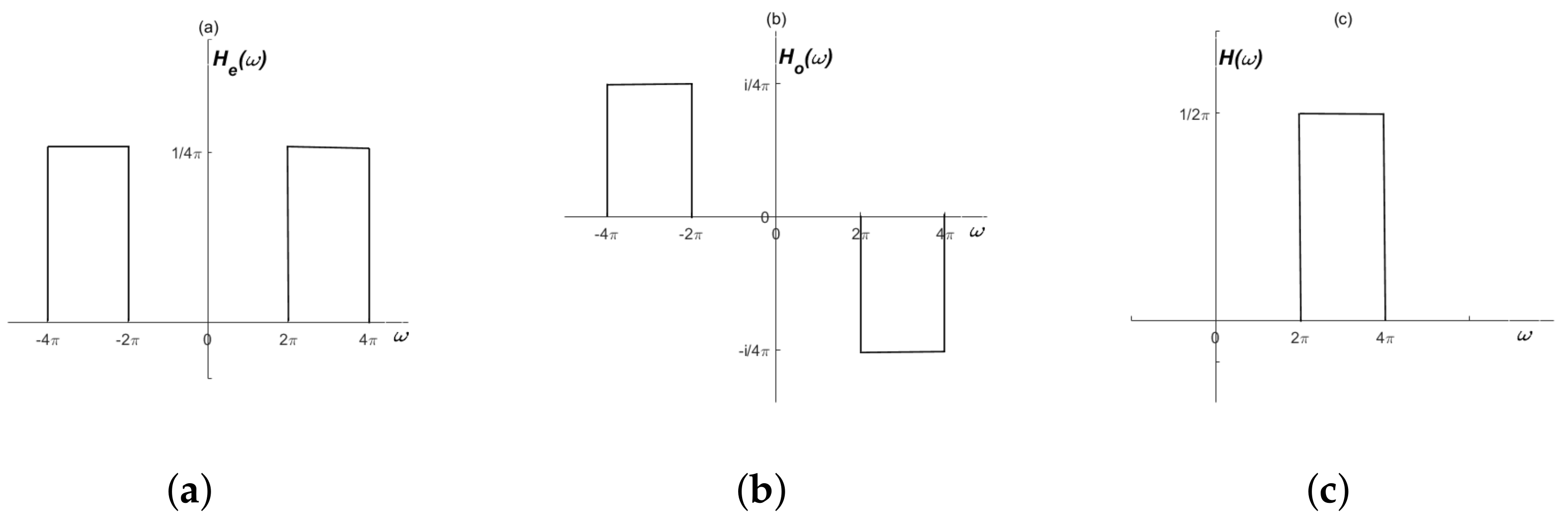
Harmonic wavelets are complex wavelets defined in the Fourier domain. It is consists of an even function (see Figure 1a) as the real part and an odd function (see Figure 1b) as the imaginary part, which are defined by
Combining and , we get the harmonic function
From Label (1), we have
This is shown in Figure 1c.
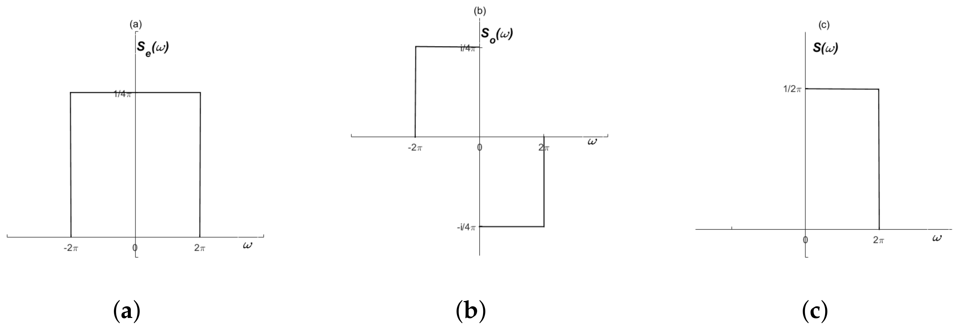
The corresponding scaling function S is given in the same way, and the even and odd functions are defined as
so that, from Label (4),
Therefore, we have
shown in Figure 2.
Then, the shifting and scaling of basic functions are denoted as and , which are given as
where is the scaling parameter, and is the shifting parameter. According to Label (7), the harmonic wavelet system constructs a basis of in the frequency domain; then, for , we have
where
3. The Circular-Shape Fourier Transform (CFT)
This section describes the circular-shape Fourier transform (CFT). We begin with the sampling grid in the Fourier domain, including the Cartesian coordinates (see Figure 3a) for classical Fourier transform and the pseudo-polar grid in [5] (see Figure 3b). This grid samples points of equally spaced long rays but not equally angles. In order to have a circular structure, the sampling grid in concentric circles (see Figure 3c) is designed, which has equally arc and angle in each circle. This type of sampling is consistent with the distribution of images in the frequency domain.
3.1. The Pseudo-Polar Grid
The pseudo-polar grid is given as
where
with the oversampling parameter. The nod of is on the solid line in Figure 3b and the nod of is on dotted line.
For an image u, the general discrete Fourier transform is evaluated on the Cartesian grid in the form
where , and
3.2. The Circular-Polar Grid (CPG)
In this section, the circular-polar grid (CPG) is designed (see Figure 3c), which is defined as
where and
where is the sampling number in each circle.
As can be seen from Figure 3c, the nod of is on a solid line and the nod on a dotted line belongs to . In addition, r in (17) serves as the radius and ℓ serves as the parameter of angle. is the sampling number. In the CPG coordinates, the nod has the following characteristics, for
where
and . For each fixed angle , the samples of the CPG are equally spaced in the radial direction, and, for each fixed radius r, the grid possesses the same angle. Formally,
where and are given by (19).
For an image u, the CFT of on CPG holds
and
3.3. The Choice of Weights
In the following, we present the basic condition of weights , according to (25), which satisfies that
According to the symmetry of the , the weighting function is assumed to satisfy
where four equations of (27) describe the -symmetry, -symmetry and the -symmetry.
In addition,
To avoid high complexity, we choose the weight in the form:
where
with , and .
4. The Construction of Multilevel System in Frequency Domain
In this section, we construct a new type multilevel system on in the frequency domain.
4.1. 2D Basic Harmonic Function
First, we define the 2D basic harmonic wavelet functions in the Fourier domain. For deriving convenience, the wavelet function and scaling function can be normalized in the form given by Definition 1 .
Definition 1.
The 2D harmonic basic functions are defined as
with , .
Then, the support of and are investigated, according to (3) and (6),
hold simultaneously; therefore,
Thus, the support of is given as
Similarly,
Next, the 2D scaling and shifting of and are defined.
Definition 2.
The 2D scaling and shifting of harmonic basic functions in the frequency domain are defined as
with .
4.2. The Polar Harmonic Multilevel System in the Frequency Domain (PHMS) on CPG
In this section, we give the definition of the polar harmonic multilevel system (PHMS) defined on CPG.
Definition 3.
The 2D PHMS on CPG is defined as
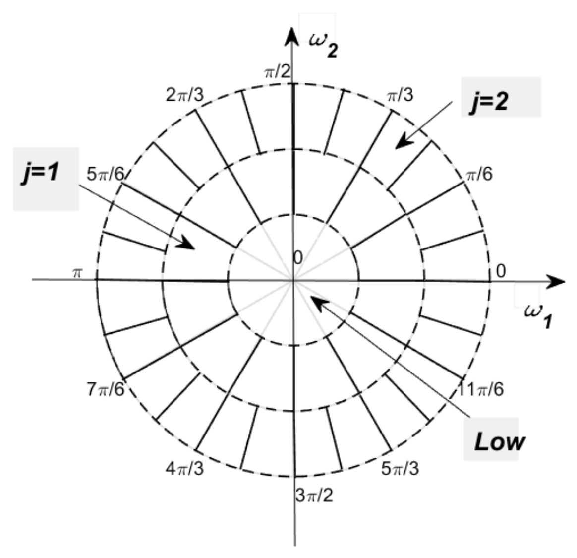
where , , and are given in (36). The level parameter , the shifting parameter is related to j, and we defined the with .
From , we have subbands in each level j, in order to reduce the overlap, we choose subbands; then, the PHMS constructs a partition of the Fourier domain. We displayed the PHMS structure in Figure 4.
For a signal or image u, the corresponding PHMS transform in the frequency domain can be defined as
with , , where is the of u, defined in (22). In addition, is the dot product, and the matrix is defined as
Theorem 1.
The discrete polar harmonic multilevel system PHMS defined on CPG forms a framelet of .
According to the framelet defined in [18], for the signal in (38),
where is the constant; therefore, PHMS forms a framelet of .
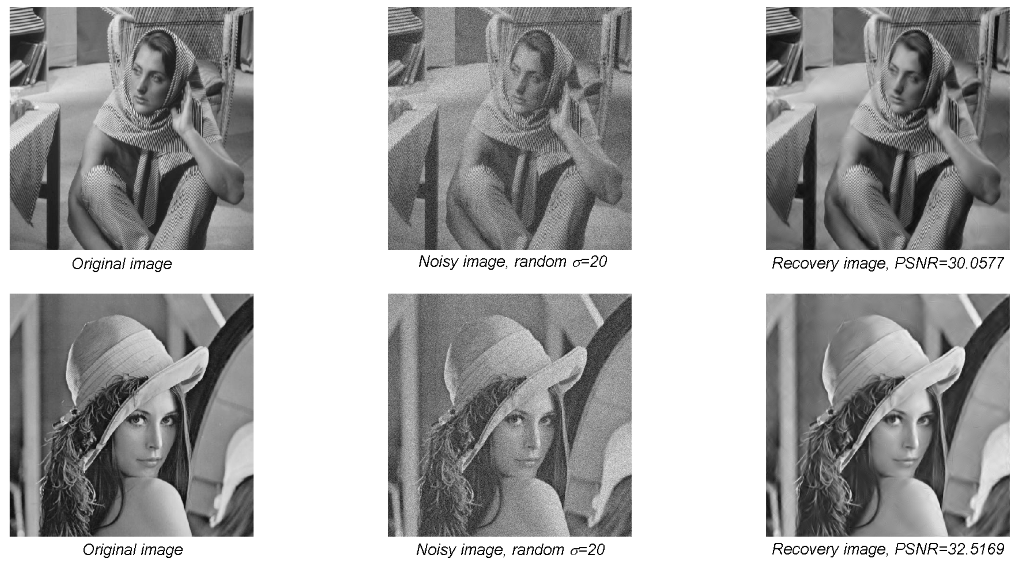
Then two denoising reconstruction tests of PHMS are shown in Figure 5.
5. Quantitative Test Measures
In the following, several performance measures are introduced to test the quality of the . The quality measure is the Monte Carlo estimate for the different operator norm by generating a sequence of five random images on for with standard normally distributed entries.
- Isometry of :
- (a)
- Closeness to tight:
- (b)
- Quality of preconditioning.
- Tight Frame Property: The operator norm , which is defined as
- Robustness:
- (a)
- Thresholding: Let u be the regular sampling of a Gaussian function with mean 0 and variance 512 on generating an image. Two types of robustness are considered, for , and .
- :
- discards percent of coefficient, with .
- :
- keeps the absolute value of coefficients bigger than with m is the maximal absolute value of all coefficients, where .
- (b)
- Quantization: The quality measure is given as where , and .
6. Test Results
In this section, the test results of on for quantitative measure in (1)–(3) are shown.
First the performance with respect to quantitative measures in , are presented in Table 1.
From Table 1, the error of tightness for the transform is about 0.1, which confirms that the multilevel system is indeed not a tight frame. The main reason is the redundancy of the multilevel structure due to the radius in (36). The quantity and suggests that the circular-polar Fourier transform provides good properties in terms of isometry, which allows us to employ the conjugate gradient method to compute the inverse of . The weight w should also be chosen carefully.
Second, the robustness measurements in displayed in Table 2:
Table 2 shows the robustness of . Even discarding of the coefficients, the image still can be recovered with error . The second row suggests that just the coefficient greater than thresholding value can give a good reconstruction with . In the third row, the quantization of robustness is displayed.
7. Conclusions
In this work, we developed and implemented a polar harmonic multilevel system on the circular-polar grid based on the multiscale theory, and testified to the performance of the in four different quantitative measures, which suggests that the transform is suitable for the circular-shape Fourier transform. Another advantage of the is that the circular low frequency region in the frequency domain is consistent with the image spectrum distribution, which can process the multilevel structure more effectively.
Acknowledgments
The first author Guomin Sun is very grateful to the China Scholarship Council for funding the first author visiting the University of Tuscia. This work was supported by the National Natural Science Foundation of China under Grant 11271001, Grant 61370147, and Grant 61573085.
Author Contributions
Guomin Sun and Carlo Cattani designed the circular multilevel system and performed the experiments, Jinsong Leng analyzed the results. Guomin Sun and Carlo Cattani wrote the paper. All authors have read and approved the final manuscript.
Conflicts of Interest
The authors declare no conflict of interest.
Abbreviations
The following abbreviations are used in this manuscript:
| CPG | Circular-polar grid |
| MRA | Multiresolution analysis |
| CFT | Circular-shape Fourier transform |
| CMS | Circular-shape directional multilevel system |
| PHMS | Polar harmonic multilevel system |
References
- Mallat, S.G. A Theory for Multiresolution Signal Decomposition: The Wavelet Representation. IEEE Trans. Pattern Anal. Mach. Intell. 1989, 11, 674–693. [Google Scholar] [CrossRef]
- Leng, J.; Huang, T.; Jing, Y.; Jiang, W. A Study on Conjugate Quadrature Filters. EURASIP J. Adv. Signal Process. 2011, 2011, 2317–2329. [Google Scholar] [CrossRef]
- Leng, J.; Cheng, Z.; Huang, T.; Lai, C. Construction and properties of multiwavelet packets with arbitrary scale and the related algorithms of decomposition and reconstruction. Comput. Math. Appl. 2006, 51, 1663–1676. [Google Scholar] [CrossRef]
- Leng, J.; Huang, T.; Fu, Y. Construction of bivariate nonseparable compactly supported biorthogonal wavelets. In Proceedings of the International Conference on Machine Learning and Cybernetics IEEE, Kunming, China, 12–15 July 2008. [Google Scholar]
- Averbuch, A.; Coifman, R.R.; Donoho, D.L.; Israeli, M.; Shkolnisky, Y. A Framework for Discrete Integral Transformations I-The Pseudopolar Fourier Transform. Siam J. Sci. Comput. 2007, 30, 764–784. [Google Scholar] [CrossRef]
- Bailey, D.H.; Swarztrauber, P.N. The Fractional Fourier Transform and Applications. SIAM Rev. 1991, 33, 389–404. [Google Scholar] [CrossRef]
- Rabiner, L.R. Chirp Z-transform algorithm. IEEE Trans. Audio Electroacoust. 1969, 17, 86–92. [Google Scholar] [CrossRef]
- Candes, E.J.; Donoho, D.L. New tight frames of curvelets and optimal representations of objects with smooth singularities. Commun. Pure Appl. Math. 2004, 57, 219–266. [Google Scholar] [CrossRef]
- Do, M.N.; Vetterli, M. The contourlet transform: an efficient directional multiresolution image representation. IEEE Trans. Image Process. 2005, 14, 2091–2106. [Google Scholar] [CrossRef] [PubMed]
- Kutyniok, G.; Shahram, M.; Zhuang, X. ShearLab: A Rational Design of a Digital Parabolic Scaling Algorithm. Siam J. Imaging Sci. 2011, 5, 1291–1332. [Google Scholar] [CrossRef]
- Kutyniok, G. Shearlets. In Applied and Numerical Harmonic Analysis; Springer: Birkhauser Basel, Berlin, Germany, 2012. [Google Scholar]
- Newland, D.E. Harmonic Wavelet Analysis. Proc. R. Soc. Math. Phys. Eng. Sci. 1993, 443, 203–225. [Google Scholar] [CrossRef]
- Cattani, C. Harmonic wavelets towards solution of nonlinear PDE. Comput. Math. Appl. 2005, 50, 1191–1210. [Google Scholar] [CrossRef]
- Cattani, C. Fractals Based on Harmonic Wavelets. In Proceedings of the International Conference on Computational Science and Its Applications, Seoul, South Korea, 29 June–2 July 2009; Springer: Berlin, Heidelberg, 2009; pp. 729–744. [Google Scholar]
- Cattani, C. Harmonic wavelet approximation of random, fractal and high frequency signals. Telecommun. Syst. 2010, 43, 207–217. [Google Scholar] [CrossRef]
- Haar, A. Zur Theorie der orthogonalen Funktionensysteme. Math. Ann. 1911, 71, 38–53. [Google Scholar] [CrossRef]
- Duan, X.; Leng, J.; Cattani, C.; Li, C. A Shannon-Runge-Kutta-Gill Method for Convection-Diffusion Equations. Math. Probl. Eng. 2013, 46, 532–546. [Google Scholar] [CrossRef]
- Cai, J.; Ji, H.; Liu, C.; Shen, Z. Framelet. IEEE Trans. Image Process. 2012, 21, 562–572. [Google Scholar] [PubMed]
Figure 1.
The harmonic wavelet function. (a) the even part ; (b) the odd part ; (c) the harmonic wavelet function .
Figure 1.
The harmonic wavelet function. (a) the even part ; (b) the odd part ; (c) the harmonic wavelet function .

Figure 2.
The harmonic scaling function. (a) the even part ; (b) the odd part ; (c) the scaling function .
Figure 2.
The harmonic scaling function. (a) the even part ; (b) the odd part ; (c) the scaling function .

Figure 3.
Three different grids.
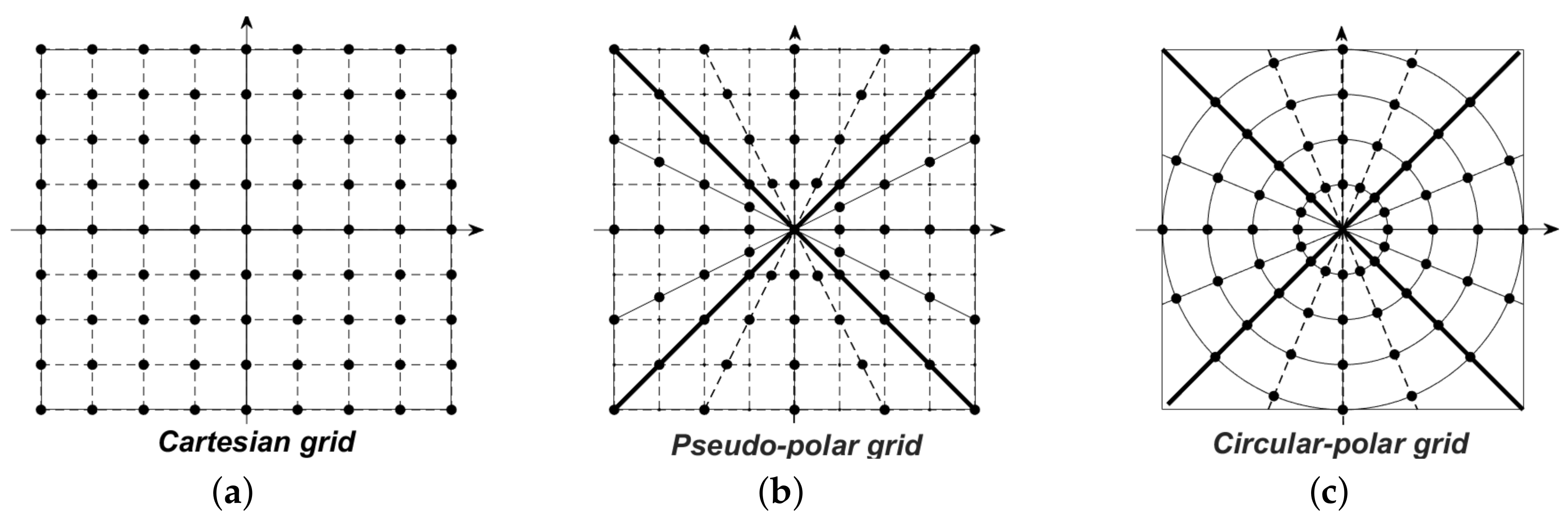
Figure 4.
The polar harmonic multilevel system (PHMS) in the Fourier domain , and .

Figure 5.
Recovery results by PHMS with scale , the random noise level .

Table 1.
Results of Labels (1)–(2).
| 0.00946092 | 1.9342627 | 0.1036731 |
Table 2.
Results of Label .
| 3.6 × 10 | 1.7 × 10 | 5.9 × 10 | 2.1 × 10 | 0.9 × 10 | |
| 0.009 | 0.063 | 0.103 | 0.172 | 0.197 | |
| 0.051 | 0.065 | 0.083 | 0.126 | 0.143 |
© 2018 by the authors. Licensee MDPI, Basel, Switzerland. This article is an open access article distributed under the terms and conditions of the Creative Commons Attribution (CC BY) license (http://creativecommons.org/licenses/by/4.0/).
Share and Cite
MDPI and ACS Style
Sun, G.; Leng, J.; Cattani, C. A Framework for Circular Multilevel Systems in the Frequency Domain. Symmetry 2018, 10, 101. https://doi.org/10.3390/sym10040101
AMA Style
Sun G, Leng J, Cattani C. A Framework for Circular Multilevel Systems in the Frequency Domain. Symmetry. 2018; 10(4):101. https://doi.org/10.3390/sym10040101
Chicago/Turabian StyleSun, Guomin, Jinsong Leng, and Carlo Cattani. 2018. "A Framework for Circular Multilevel Systems in the Frequency Domain" Symmetry 10, no. 4: 101. https://doi.org/10.3390/sym10040101
Note that from the first issue of 2016, this journal uses article numbers instead of page numbers. See further details here.