Multicriteria Decision Making Based on Generalized Maclaurin Symmetric Means with Multi-Hesitant Fuzzy Linguistic Information

Abstract

In multicriteria decision making (MCDM), multi-hesitant fuzzy linguistic term sets (MHFLTSs) can eliminate the limitations of hesitant fuzzy linguistic term sets (HFLTSs) and hesitant fuzzy linguistic sets (HFLSs), and emphasize the importance of a repeated linguistic term (LT). Meanwhile, there is usually an interrelation between criteria. The Maclaurin symmetric mean (MSM) operator can capture the interrelationships among multi-input arguments. The purpose of this paper is to integrate MHFLTSs with MSM operators and to solve MCDM problems. Firstly, we develop the generalized MSM operator for MHFLTSs (MHFLGMSM), the generalized geometric MSM operator for MHFLTSs (MHFLGGMSM), the weighted generalized MSM operator for MHFLTSs (WMHFLGMSM) and the weighted generalized geometric MSM operator for MHFLTSs (WMHFLGGMSM), respectively. Then, we discuss their properties and some special cases. Further, we present a novel method to deal with MCDM problems with the MHFLTSs based on the proposed MSM operators. Finally, an illustrative example about how to select the best third-party logistics service provider is supplied to demonstrate the practicality and reliability of the proposed approaches in comparison with some existing approaches.

1. Introduction

Because human preferences are inherently vague, it is more suitable to deal with uncertainty and imprecise information by linguistic terms (LTs). For example, when evaluating customer satisfaction of a service or product, experts are inclined to select some LTs such as “poor”, “good” or “excellent”, etc., to give their evaluation of the criteria. Since Zadeh [1] presented the fuzzy linguistic technique in 1975, which utilized linguistic variables (LVs) to describe qualitative information, some methods based on LVs have been utilized in a number of areas, such as supply chain management [2], qualify function deploy [3], health care system [4], housing marker [5], risk evaluation [6], etc.

Generally, if the qualitative information is only represented by a single LT, it might sometimes not accurately reflect what it means. When the decision-making problems become more ambiguous, the experts might be hesitant among several LTs and need two or more LTs to express their preference. Based on hesitant fuzzy set (HFS), Rodríguez et al. [7,8] defined a hesitant fuzzy LT set (HFLTS), which is a set with ordered consecutive LTs. In real applications, experts can give several possible LTs instead of a single LT to evaluate the criteria. Although HFLTS improves the previous linguistic approaches, it is still difficult to express the hesitance preference of experts only by consecutive LTs. In addition, there are some limitations in the calculation of HFLTS and this will be illustrated in Section 2 of this paper. Thus, hesitant fuzzy linguistic sets (HFLSs), as an extension of HFLTS, were produced, which allow for inconsecutive LTs. However, in practice, when multi-persons give the same LT in assessment information, this LT is handled as one time by default and the significance of repeated LTs is neglected. Since the evaluation values $\left\{x_1,x_2,x_3\right\}$, $\left\{x_1,x_2,x_2,x_3\right\}$ and $\left\{x_1,x_2,x_2,x_2,x_3\right\}$ are not equivalent to each other, the repeated occurrence of $x_2$ can convey importance or a certain special meaning. In addition, the LVs provided by experts generally fluctuate in evaluation period [9]. So, MHFLTS [10] was proposed based on multi-HFSs to solve the mentioned problems, and each multi-hesitant LT element (MHFLTE) can contain inconsecutive and repeated LTs. Based on the MHFLTS, one expert can assess an alternative under specific criteria by one or several arbitrary LTs, and the assessment values from the different experts, can be collected, and the frequency of a LT can be expressed in the assessment information [11]. In a word, MHFLTS is more energetic than the HFLTS and HFLS, and it can be applied to present the hesitance linguistic information by multi-repeated LTs in primary assessment information.

To date, many contributions have concentrated on the decision-making techniques based on HFLTSs, which are from three domains: (1) the theory of foundations, for instance, operational laws [7,8], comparative methods [12,13], distance and similarity measures [14], likelihood [15], outranking degree [16], consistency [17] or multiplicative consistency [18],correlation coefficient [19] and so on; (2) the extended multicriteria decision making (MCDM) approaches for HFLTS, such as TOPSIS [20], ELECTRE [21], VIKOR [22], TODIM [23], Entropy [24], GRA [25] and other methods, such as MACBETH [26], linear programming technique [27],Shapely [28], EDAS [29], Fuzzy Petri Net [30] and so on; (3) the MCDM techniques based on aggregation operators of HFLS. The MCDM methods based on aggregation operators can acquire the comprehensive values of alternatives by aggregating all attribute values, and then rank the alternatives. Obviously, they have more superiority than the traditional MCDM methods, and it is meaningful to research the aggregation operators and then to solve the MCDM problems.

As an important tool for information fusion, a great number of research achievements about aggregation operators of HFLS have been produced. Wang et al. [31] presented a 2-tuple linguistic aggregation operator for MHFLTEs; Wu [32] applied possibility distribution to develop the weighted average (WA) operator for HFLSs (HFLWA) and the ordered WA operator (OWA) for HFLSs (HFLOWA). Gou et al. [33] developed the hesitant fuzzy linguistic BM operator for HFLSs (HFLBM) and the weighted HFLBM operator (WHFLBM). Zhu et al. [34] investigated some linguistic hesitant fuzzy power aggregation (LHFPA) operators. Wang et al. [35] proposed the cloud WA (CWA) operator, cloud OWA (COWA) operator, and cloud hybrid arithmetic (CHA) operator for LVs. Liu et al. [36] investigated prioritized WA operator for HIFLSs (HIFLPWA) and prioritized weighted geometric operator for HIFLSs (HIFLPWG). However, these operators for HFLTSs do not pay attention to the interrelation among input arguments.

MSM was proposed by Maclaurin [37] and was further developed by Detemple and Robertson [38], which has distinct advantage, i.e., it can deal with the interrelationship among multi-inputs, however Bonferroni mean (BM) operator and Heronian mean (HM) operator can only consider the correlation between two arguments. Consequently, based on its main advantage of more flexible and robust in information fusion, the related research achievements of MSM operator have been quite fruitful. Liu and Zhang [39] introduced some MSM operator for single-valued trapezoidal neutrosophic numbers. Yu et al. [33] developed the MSM operator for HFLSs and the weighted MSM operator for HFLSs. Liu and Qin [40] extended the MSM operator for linguistic intuitionistic fuzzy numbers (LIFNs). Qin and Liu [41] investigated the dual MSM (DMSM) operator and extended the DMSM operator to uncertain LVs. Moreover, the MSM operators were also applied to handle the 2-tuple linguistic information [42] and single-valued neutrosophic linguistic information [43] and so on.

However, research about MHFLTSs and their application in MCDM is limited. Wang et al. [31] presented a generalized 2-tuple linguistic WA operator and a generalized 2-tuple linguistic OWA to deal with MHFLTSs. Afterwards, a likelihood-based TODIM method based on the MHFLTSs for evaluation in logistics outsourcing was also proposed [11]. Then, Wang et al. [10] further developed the HM and prioritized operators to solve the MCDM problem with the MHFLTSs. Liu and Teng [44] proposed some normal neutrosophic number Heronian Mean operators for solving multiple attribute group decision making problems. However, because MHFLTSs can describe inconsecutive and repeated LTs and MSM aggregation operator can process the correlations among multi-inputs, to develop some MSM operators to deal with MHFLTSs is an important work. So, the aim of this paper is to establish some MSM operators for MHFLTSs and use them to solve the MCDM problem in which the attributes take the form of MHFLTSs.

This paper is organized as follows. Section 2 reviews and discusses some basic concepts and theories. Section 3 proposes some multi-hesitant fuzzy linguistic generalized MSM operators, including the generalized MSM operator for MHFLTSs (MHFLGMSM), the generalized geometric MSM operator for MHFLTSs (MHFLGGMSM), the weighted generalized MSM operator for MHFLTSs (WMHFLGMSM) and the weighted generalized geometric MSM operator for MHFLTSs (WMHFLGGMSM), and studies some properties and some particular examples of these operators. Section 4, outlines an MCDM approach based on the proposed aggregation operators. Section 5 gives a case to verify the availability of the presented methods. Section 6 presents a few conclusions.

2. Preliminaries

In this part, the definitions of HFLTSs, HFLSs and MHFLTEs are briefly reviewed and their corresponding operations are given. Subsequently, the linguistic scale function (LSF) and score function of MHFLTS were given.

2.1. HFLTSs

Assume that $S=\left\{s_i|i=0,1,2,\cdots ,2g,g\in N\right\}$ is a LT set (LTs) with odd cardinality, where s_i is called a LV. Then the following requirements must be satisfied [2]:

(1)

The set is ordered: $\alpha >\beta \iff s_{\alpha }>s_{\beta }$;

(2)

There is a negation operator: $neg\left(s_{\alpha }\right)=s_{2g-\alpha }$.

Definition 1.

Let $S=\left\{s_i|i=0,1,2,\cdots ,2g,g\in N\right\}$, then a HFLTS $H_s$ is an ordered finite consecutive LTs of S [31].

Definition 2.

Let $H_s$, $H_s^1$ and $H_s^2$ be any three HFLTSs on S [31]. Then we have

(1) 

The upper bound $h_{s^{+}}:h_{s^{+}}=\max \left\{h_{\tau }|h_{\tau }\in H_s\right\}$; and the lower bound $h_{s^{-}}$ of H_s: $h_{s^{-}}=\min \left\{h_{\tau }|h_{\tau }\in H_s\right\}$ and $h_{s^{-}}\le h_{s^{+}}$;

(2) 

The intersection between $H_s^1$ and $H_s^2$ : $H_s^1{\cap }_s{H}_s^2=\left\{h_{\tau }|h_{\tau }\in H_s^1\mathrm{and}{h}_{\tau }\in H_s^2\right\}$;

(3) 

The union of $H_s^1$ and $H_s^2$ : $H_s^1{\cup }_s{H}_s^2=\left\{h_{\tau }|h_{\tau }\in H_s^1\mathrm{or}{h}_{\tau }\in H_s^2\right\}$.

Example 1.

Assume that $S=\left\{s_i|i=0,1,2,\cdots ,8\right\}$, $H_s^1=\left\{s_5,s_6\right\}$, $H_s^2=\left\{s_3,s_4,s_5\right\}$ and $H_s^3=\left\{s_1,s_2,s_3\right\}$ are three HFLTSs on S. Then, we get:

(1) 

$h_{s^{+}}^1=\left\{s_6\right\}$ and $h_{s^{-}}^1=\left\{s_5\right\}$;

(2) 

$H_s^1{\cap }_s{H}_s^2=\left\{s_5\right\}$ and $H_s^1{\cup }_s{H}_s^3=\left\{s_1,s_2,s_3,s_5,s_6\right\}$.

Obviously, the union of $H_s^1$ and $H_s^3$ is not a HFLTS because the HFLTS must be consecutive LTs. So, the HFLTSs were extended to HFLSs.

2.2. HFLSs

In order to preserve the provided information, the LTs S is developed to a successive LTs $\overline{S}=\left\{s_k|k\in \left[0,2g\right]\right\}$. If $s_k\in S$, then $s_k$ is named the original LT; if not so, $s_k$ is named the virtual LT which has no practical meaning and only it is used to operational process.

Definition 3.

Let X be a reference set and $\overline{S}=\left\{s_k|k\in \left[0,2g\right]\right\}$. Then a HFLS $H_{LS}$ on X can be defined in terms of a function $H_{LS}$ that returns a subset of $\overline{S}$ [32].

For simple and convenient, $h_{LS}\left(x\right)=h_{LS}$ is called a HFLE.

Definition 4.

Let $\overline{S}=\left\{s_k|k\in \left[0,2g\right]\right\}$ be a LTs, $h_{LS}$, $h_{LS}^1$ and $h_{LS}^2$ be three HFLEs on $\overline{S}$ and $\lambda \in \left[0,1\right]$, $I\left(s_k\right)=k$ [32]. Thus, the operations can be defined as follows:

$$h_{LS}^1\oplus h_{LS}^2={\cup }_{h_{{\tau }^1}\in h_{LS}^1,h_{{\tau }^2}\in h_{LS}^2}\left\{h_{{\tau }^1}\oplus h_{{\tau }^2}\right\}={\cup }_{h_{{\tau }^1}\in h_{LS}^1,h_{{\tau }^2}\in h_{LS}^2}\left\{s_{I\left(h_{{\tau }^1}\right)+I\left(h_{{\tau }^2}\right)}\right\}$$

(1)

$$h_{LS}^1\otimes h_{LS}^2={\cup }_{h_{{\tau }^1}\in h_{LS}^1,h_{{\tau }^2}\in h_{LS}^2}\left\{h_{{\tau }^1}\otimes h_{{\tau }^2}\right\}={\cup }_{h_{{\tau }^1}\in h_{LS}^1,h_{{\tau }^2}\in h_{LS}^2}\left\{s_{I\left(h_{{\tau }^1}\right)\times I\left(h_{{\tau }^2}\right)}\right\}$$

(2)

$$\lambda h_{LS}={\cup }_{h_{\tau }\in h_{LS}}\left\{\lambda h_{\tau }\right\}={\cup }_{h_{\tau }\in h_{LS}}\left\{s_{\left(\lambda I\left(h_{\tau }\right)\right)}\right\}$$

(3)

$${\left(h_{LS}\right)}^{\lambda }={\cup }_{h_{\tau }\in h_{LS}}\left\{{\left(h_{\tau }\right)}^{\lambda }\right\}={\cup }_{h_{\tau }\in h_{LS}}\left\{s_{{\left(I\left(h_{\tau }\right)\right)}^{\lambda }}\right\}$$

(4)

Example 2.

Suppose that $\overline{S}=\left\{s_k|k\in \left[0,8\right]\right\}$ and $h_{LS}^1$, $h_{LS}^2$, $h_{LS}^3$ are three HFLEs on $\overline{S}$. $h_{LS}^1=\left\{s_5,s_6\right\}$, $h_{LS}^2=\left\{s_3,s_4,s_5\right\}$ and $h_{LS}^3=\left\{s_1,s_2,s_3\right\}$. Then, $h_{LS}^1\oplus h_{LS}^2=\left\{s_8,s_9,s_{10},s_{11}\right\}$, $h_{LS}^1\otimes h_{LS}^3=\left\{s_5,s_6,s_{10},s_{12},s_{15},s_{18}\right\}$.

The results obtained by Definition 4 have exceed the domain of $\overline{S}$. Many elements based on the subscript of LTs in $h_{LS}^1\oplus h_{LS}^2$ and $h_{LS}^1\otimes h_{LS}^3$ do not exist in $\overline{S}$.

Definition 5.

Let $\overline{S}=\left\{s_k|k\in \left[0,2g\right]\right\}$ be a LTs and $h_{LS}=\left\{h_{\tau }|h_{\tau }\in \overline{S}\right\}$ be a HFLE on $\overline{S}$ [33]. The score function of $h_{LS}$ is

$$S\left(h_{LS}\right)=\frac{1}{\#h_{LS}}{\displaystyle {\sum }_{h_{\tau }\in h_{LS}}\frac{I\left(h_{\tau }\right)}{2g}}$$

(5)

where $\#h_{LS}$ indicates the count of elements in $h_{LS}$. $h_{LS}^1$, $h_{LS}^2$ are two arbitrary HFLEs, if $S\left(h_{LS}^1\right)>S\left(h_{LS}^2\right)$ then $h_{LS}^1>h_{LS}^2$ , and if $S\left(h_{LS}^1\right)=S\left(h_{LS}^2\right)$ then $h_{LS}^1=h_{LS}^2$.

Example 3.

Assume that $\overline{S}=\left\{s_k|k\in \left[0,8\right]\right\}$ and $h_{LS}^1$, $h_{LS}^2$ are two HFLEs on $\overline{S}$. $h_{LS}^1=\left\{s_2,s_4,s_6\right\}$, $h_{LS}^2=\left\{s_2,s_6\right\}$, $S\left(h_{LS}^1\right)=S\left(h_{LS}^2\right)=0.5$, then $h_{LS}^1=h_{LS}^2$. However, this comparison result is insufficient due to the existence of $s_4$. Therefore, it is essential to give some revisions.

2.3. MHFLTS

Although the definitions of HFLTS and HFLS have been widely and consistently used, the frequency of one repeated LT is assigned to be one time and the operations are contradictory to the definitions. Thus, a further extended definition of them is proposed in this section.

Definition 6.

Suppose X is a reference set, a multi-HFS on X can be defined about a function $h_E$ that returns a multi-subset of values in $\left[0,1\right]$ [31].

Definition 7.

Suppose X is a reference set and $\overline{S}=\left\{s_k|k\in \left[0,2g\right]\right\}$ is a LTs. Then a MHFLTS H on X is defined about a function h that returns an ordered finite multi-subset of $\widehat{S}$, denoted by [31]:

$$H=\left\{\langle x,h\left(x\right)\rangle |x\in X\right\}$$

(6)

where h(x) indicates the possible membership degrees of the element $x\in X$ to the set X. For simple and convenient, h(x) = h is a MHFLTE and $\widehat{H}$ is the set of all MHFLTEs. There is the strong possibility that the virtual LTs of h exist in $\overline{S}$ but not in S.

Essentially, MHFLTSs are a development of HFLTSs and HFLSs. If h is a set of successive LTs and no duplicate LT, then h is a HFLTSs. If h is a set of discrete LTs with no duplicate LT, then h is a HFLS. Therefore, all the operations and approaches on MHFLTSs can be applied to HFLTSs and HFLSs because they are both special cases of MHFLTSs.

Definition 8.

Let $\overline{S}=\left\{s_k|k\in \left[0,2g\right]\right\}$ be a LTs. The LSF $\vartheta :\overline{S}\to R^{+}$ is a strictly monotone increasing and continuous function satisfying $\vartheta \left(0\right)=0$ and $\vartheta \left(2g\right)=1$. The inverse function of $\vartheta$ exists and is denoted by ${\vartheta }^{-1}(\cdot )$. Then ${\vartheta }^{-1}\left(\delta \right)=h_{\tau }$, where $h_{\tau }\in \overline{S}$ and $\delta \in R^{+}$ [41,42].

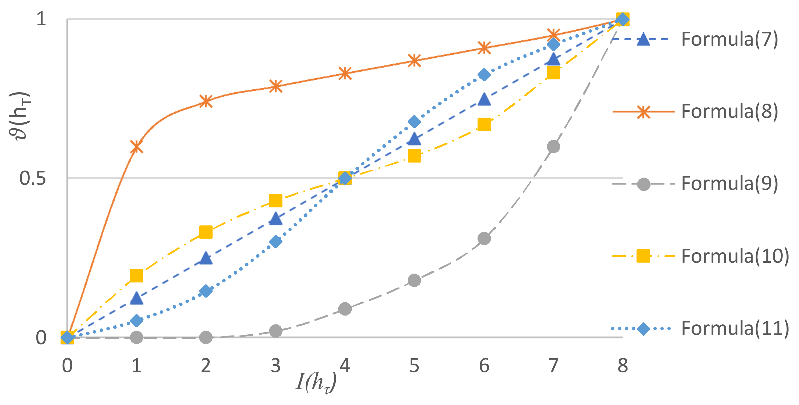
There are five normal LSFs which are shown as below.

$$\vartheta \left(h_{\tau }\right)=\frac{I\left(h_{\tau }\right)}{2g}I\left(h_{\tau }\right)\in \left[0,2g\right]$$

(7)

$$\vartheta \left(h_{\tau }\right)={\left(\frac{I\left(h_{\tau }\right)}{2g}\right)}^{g}I\left(h_{\tau }\right)\in \left[0,2g\right]$$

(8)

$$\vartheta \left(h_{\tau }\right)={\left(\frac{I\left(h_{\tau }\right)}{2g}\right)}^{\frac{1}{g}}I\left(h_{\tau }\right)\in \left[0,2g\right]$$

(9)

$$\vartheta \left(h_{\tau }\right)=\{\begin{array}{ll}\frac{a^g-a^{g-I\left(h_{\tau }\right)}}{2\left(a^g-1\right)}& \left(I\left(h_{\tau }\right)\in \left[0,g\right]\right)\\ \frac{a^g+a^{I\left(h_{\tau }\right)-g}-2}{2\left(a^g-1\right)}& \left(I\left(h_{\tau }\right)\in \left[0,g\right]\right)\end{array}$$

(10)

$$\vartheta \left(h_{\tau }\right)=\{\begin{array}{ll}\frac{g^a-{\left(g-I\left(h_{\tau }\right)\right)}^a}{2g^{\alpha }}& \left(I\left(h_{\tau }\right)\in \left[0,g\right]\right)\\ \frac{g^{\beta }+{\left(I\left(h_{\tau }\right)-g\right)}^{\beta }}{2g^{\alpha }}& \left(I\left(h_{\tau }\right)\in \left[0,g\right]\right)\end{array},\mathrm{where}\alpha ,\beta \in (0,1]$$

(11)

A great quantity of experiment research has proven the value of a in Equation (10) lies in the interval [1.36, 1.4]. Suppose $g=4$, $a=1.4$ and $\alpha =\beta =0.8$, the character of Equations (7)–(11) can be shown in Figure 1.

The Equation (10) is regarded as one representative among all Equations for ${\vartheta }^{-1}(\cdot )$, thus we choose it to deal with the MHFLTEs in this paper.

2.4. Basic Operations of MHFLTS

Definition 9.

Let h₁ and h₂ be any two MHFLTEs on $\overline{S}$. Then, we can give the following operations.

$$h_1\oplus h_2=\left\{{\vartheta }^{-1}\right(\vartheta \left(h_{\tau 1}\right)+\vartheta \left(h_{\tau 2}\right)\left)\right|h_{\tau 1}\in h_1,h_{\tau 2}\in h_2\}$$

(12)

$$h_1\otimes h_2=\left\{{\vartheta }^{-1}\right(\vartheta \left(h_{\tau 1}\right)+\vartheta \left(h_{\tau 2}\right)\left)\right|h_{\tau 1}\in h_1,h_{\tau 2}\in h_2\}$$

(13)

$$\lambda h_1=\left\{{\vartheta }^{-1}\right(\lambda \vartheta \left(h_{\tau }\right)\left)\right|h_{\tau }\in h_1\}$$

(14)

$${\left(h_1\right)}^{\lambda }=\left\{{\vartheta }^{-1}{\left(\vartheta \left(h_{\tau }\right)\right)}^{\lambda }\right|h_{\tau }\in h_1\}$$

(15)

Definition 10.

Let h, h₁, h₂ be arbitrary MHFLTEs on $\overline{S}$. Then we give the score function of h as follows [31]:

$$S\left(h\right)=\frac{1}{\#h}{\displaystyle {\sum }_{h_{\tau }\in h}\vartheta \left(h_{\tau }\right)}$$

(16)

and the variance function of h as follows:

$$V\left(h\right)=\frac{1}{\#h}{{\displaystyle {\sum }_{h_{\tau }\in h}\left(\vartheta \left(h_{\tau }\right)-S\left(h\right)\right)}}^2$$

(17)

where #h denotes the count of elements in h. Then the comparison rules for MHFLTEs can be re-defined as follows:

(1) 

If $\vartheta \left(h_1^{-}\right)>\vartheta \left(h_1^{+}\right)$, then $h_1$ is strictly greater than $h_2$, denoted by $h_1>h_2$;

(2) 

If $S\left(h_1\right)>S\left(h_2\right)$, then $h_1$ is greater than $h_2$, denoted by $h_1>h_2$; If $S\left(h_1\right)=S\left(h_2\right)$, and $V\left(h_1\right)<V\left(h_2\right)$, then $h_1>h_2$; If $S\left(h_1\right)=S\left(h_2\right)$, and $V\left(h_1\right)=V\left(h_2\right)$, then $h_1=h_2$.

2.5. MSM Operator

Definition 11.

Let $a_i\left(i=1,2,\cdots ,n\right)$ be a group of positive real values and $m=1,2,\cdots ,n$ [43]. If

$$MS{M}^{\left(m\right)}\left(a_1,a_2,\cdots ,a_n\right)={\left(\frac{{\displaystyle {\sum }_{1\le i_1<\cdots <i_m\le i_n}{\displaystyle {\prod }_{j=1}^m{a}_{i_j}}}}{C_n^m}\right)}^{\frac{1}{m}}$$

(18)

Then $MS{M}^{\left(m\right)}$ is called the MSM operator where $\left(i_1,i_2,\cdots ,i_m\right)$ traversal all the combination of $\left(1,2,\cdots ,n\right)$, $C_n^m$ is the binominal coefficient.

It is clear that the $MS{M}^{\left(m\right)}$ has the following properties:

(1)

Idempotency. $MS{M}^{\left(m\right)}\left(a,a,\cdots ,a\right)=a$;

(2)

Monotonicity. $MS{M}^{\left(m\right)}\left(a_1,a_2,\cdots ,a_n\right)\le MS{M}^{\left(m\right)}\left(b_1,b_2,\cdots ,b_n\right)$, if $a_i<b_i$ for all i;

(3)

Boundedness. $\min \left\{a_1,a_2,\cdots ,a_n\right\}\le MS{M}^{\left(m\right)}\left(a_1,a_2,\cdots ,a_n\right)\le \max \left\{a_1,a_2,\cdots ,a_n\right\}$.

Especially, if m = 1, then the $MS{M}^{\left(1\right)}$ reduces to the WA operator as follows:

$$MS{M}^{\left(1\right)}\left(a_1,a_2,\cdots ,a_n\right)=\frac{{\displaystyle {\sum }_{1\le i_1\le i_n}{a}_i}}{n}$$

(19)

If m = 2, then the $MS{M}^{\left(2\right)}$ reduces to a BM operator ($p=q=1$), as follows:

$$\begin{array}{l}MS{M}^{\left(2\right)}\left(a_1,a_2,\cdots ,a_n\right)={\left(\frac{{\displaystyle {\sum }_{1\le i_1<i_2\le i_n}{\displaystyle {\prod }_{j=1}^2{a}_{i_j}}}}{C_n^2}\right)}^{\frac{1}{2}}={\left(\frac{2{\displaystyle {\sum }_{1\le i_1<i_2\le i_n}{a}_{i_1}{a}_{i_2}}}{n\left(n-1\right)}\right)}^{\frac{1}{2}}\\ ={\left(\frac{{\displaystyle {\sum }_{i,j=1,i\ne j}^n{a}_{i_1}{a}_{i_2}}}{n\left(n-1\right)}\right)}^{\frac{1}{2}}=B{M}^{1,1}\left(a_1,a_2,\cdots ,a_n\right)\end{array}$$

(20)

If m = 3, then the $MS{M}^{\left(3\right)}$ reduces to a generalized BM operator ($p=q=u=1$) as follows:

$$\begin{array}{l}MS{M}^{\left(3\right)}\left(a_1,a_2,\cdots ,a_n\right)={\left(\frac{{\displaystyle {\sum }_{1\le i_1<i_2<i_3\le i_n}{\displaystyle {\prod }_{j=1}^3{a}_{i_j}}}}{C_n^3}\right)}^{\frac{1}{3}}={\left(\frac{6{\displaystyle {\sum }_{1\le i_1<i_2\le i_n}{a}_{i_1}{a}_{i_2}{a}_{i_3}}}{n\left(n-1\right)\left(n-2\right)}\right)}^{\frac{1}{3}}\\ ={\left(\frac{{\displaystyle {\sum }_{i,j,r=1,i\ne j\ne r}^n{a}_{i_1}{a}_{i_2}{a}_{i_3}}}{n\left(n-1\right)\left(n-2\right)}\right)}^{\frac{1}{3}}=GB{M}^{1,1,1}\left(a_1,a_2,\cdots ,a_n\right)\end{array}$$

(21)

Definition 12.

Let $a_i\left(i=1,2,\cdots ,n\right)$ be a set of positive real values and $m=1,2,\cdots ,n$ [43]. If

$$GMS{M}^{\left(m,p_1,p_2,\cdots ,p_m\right)}\left(a_1,a_2,\cdots ,a_n\right)={\left(\frac{{\displaystyle {\sum }_{1\le i_1<\cdots <i_m\le i_n}{\displaystyle {\prod }_{j=1}^m{a}_{i_j}^{p_j}}}}{C_n^m}\right)}^{\frac{1}{p_1+p_2+\cdots +p_m}}$$

(22)

Then $GMS{M}^{\left(m,p_1,p_2,\cdots ,p_m\right)}$ is called the generalized MSM (GMSM) operator, where $p_1,p_2,\cdots ,p_m\ge 0$, $\left(i_1,i_2,\cdots ,i_m\right)$ traversal all the combination of $\left(1,2,\cdots ,n\right)$, $C_n^m$ is the binominal coefficient.

The $GMS{M}^{\left(m,p_1,p_2,\cdots ,p_m\right)}$ has the following properties:

Property 1.

(1) 

Idempotency. $GMS{M}^{\left(m,p_1,p_2,\cdots ,p_m\right)}\left(a,a,\cdots ,a\right)=a$;

(2) 

Monotonicity. $GMS{M}^{\left(m,p_1,p_2,\cdots ,p_m\right)}\left(a_1,a_2,\cdots ,a_n\right)\le GMS{M}^{\left(m,p_1,p_2,\cdots ,p_m\right)}\left(b_1,b_2,\cdots ,b_n\right)$, if $a_i\le b_i$ for all i;

(3) 

Boundedness. $\min \left\{a_1,a_2,\cdots ,a_n\right\}\le GMS{M}^{\left(m,p_1,p_2,\cdots ,p_m\right)}\left(a_1,a_2,\cdots ,a_n\right)\le \max \left\{a_1,a_2,\cdots ,a_n\right\}$.

Proof. 

(1)

$\begin{array}{l}GMS{M}^{\left(m,p_1,p_2,\cdots ,p_m\right)}\left(a,a,\cdots ,a\right)={\left(\frac{{\displaystyle {\sum }_{1\le i_1<\cdots <i_m\le i_n}{\displaystyle {\prod }_{j=1}^m{a}^{p_j}}}}{C_n^m}\right)}^{\frac{1}{p_1+p_2+\cdots +p_m}}={\left(\frac{{\displaystyle {\sum }_{1\le i_1<\cdots <i_m\le i_n}{a}^{p_1+p_2+\cdots +p_m}}}{C_n^m}\right)}^{\frac{1}{p_1+p_2+\cdots +p_m}}\\ ={\left(\frac{C_n^m{a}^{p_1+p_2+\cdots +p_m}}{C_n^m}\right)}^{\frac{1}{p_1+p_2+\cdots +p_m}}=a\end{array}$

(2)

Assume that m-tuple $\left(i_1,i_2,\cdots ,i_m\right)$ is given randomly, and $p_1,p_2,\cdots ,p_m\ge 0$. if $0\le a_i\le b_i$ for all $i$, then ${\displaystyle {\prod }_{j=1}^m{a}_{i_j}^{p_j}}\le {\displaystyle {\prod }_{j=1}^m{b}_{i_j}^{p_j}}$ and ${\displaystyle {\sum }_{1\le i_1<\cdots <i_m\le i_n}{\displaystyle {\prod }_{j=1}^m{a}_{i_j}^{p_j}}}\le {\displaystyle {\sum }_{1\le i_1<\cdots <i_m\le i_n}{\displaystyle {\prod }_{j=1}^m{b}_{i_j}^{p_j}}}$, therefore,

$${\left(\frac{{\displaystyle {\sum }_{1\le i_1<\cdots <i_m\le i_n}{\displaystyle {\prod }_{j=1}^m{a}_{i_j}^{p_j}}}}{C_n^m}\right)}^{\frac{1}{p_1+p_2+\cdots +p_m}}\le {\left(\frac{{\displaystyle {\sum }_{1\le i_1<\cdots <i_m\le i_n}{\displaystyle {\prod }_{j=1}^m{b}_{i_j}^{p_j}}}}{C_n^m}\right)}^{\frac{1}{p_1+p_2+\cdots +p_m}}$$

(3)

Let $a^{-}=\min \left\{a_1,a_2,\cdots ,a_n\right\}$ and $a^{+}=\max \left\{a_1,a_2,\cdots ,a_n\right\}$. According to the property of idempotency, $\min \left\{a_1,a_2,\cdots ,a_n\right\}=a^{-}=GMS{M}^{\left(m,p_1,p_2,\cdots ,p_m\right)}\left(a^{-},a^{-},\cdots ,a^{-}\right)$. According to the property of monotonicity, when $a^{-}\le a_i$ for all i, we have $GMS{M}^{\left(m,p_1,p_2,\cdots ,p_m\right)}\left(a^{-},a^{-},\cdots ,a^{-}\right)\le GMS{M}^{\left(m,p_1,p_2,\cdots ,p_m\right)}\left(a_1,a_2,\cdots ,a_n\right)$. Similarly, we also have $GMS{M}^{\left(m,p_1,p_2,\cdots ,p_m\right)}\left(a_1,a_2,\cdots ,a_n\right)\le GMS{M}^{\left(m,p_1,p_2,\cdots ,p_m\right)}\left(a^{+},a^{+},\cdots ,a^{+}\right)$.

Finally, $MS{M}^{\left(m,p_1,p_2,\cdots ,p_m\right)}\left(a_1,a_2,\cdots ,a_n\right)\le MS{M}^{\left(m,p_1,p_2,\cdots ,p_m\right)}\left(b_1,b_2,\cdots ,b_n\right)$. □

Especially, if m = 1, then the $GMS{M}^{\left(m,p_1,p_2\right)}\left(a_1,a_2,\cdots ,a_n\right)$ reduces to the generalized WA operator.

$$GMS{M}^{\left(1,p\right)}\left(a_1,a_2,\cdots ,a_n\right)={\left(\frac{{\displaystyle {\sum }_{1\le i_1\le i_n}{a}_i^p}}{n}\right)}^{\frac{1}{p}}$$

(23)

If m = 2, then the $GMS{M}^{\left(m,p_1,p_2\right)}\left(a_1,a_2,\cdots ,a_n\right)$ reduces to the BM operator as follows:

$$\begin{array}{l}GMS{M}^{\left(2,p_1,p_2\right)}\left(a_1,a_2,\cdots ,a_n\right)={\left(\frac{{\displaystyle {\sum }_{1\le i_1<i_2\le i_n}{a}_{i_1}^{p_1}{a}_{i_2}^{p_2}}}{C_n^2}\right)}^{\frac{1}{p_1+p_2}}={\left(\frac{2{\displaystyle {\sum }_{1\le i<j\le n}{a}_i^{p_1}{a}_j^{p_2}}}{n\left(n-1\right)}\right)}^{\frac{1}{p_1+p_2}}\\ ={\left(\frac{{\displaystyle {\sum }_{i,j=1,i\ne j}^n{a}_i^{p_1}{a}_j^{p_2}}}{n\left(n-1\right)}\right)}^{\frac{1}{p_1+p_2}}=B{M}^{p_1,p_2}\left(a_1,a_2,\cdots ,a_n\right)\end{array}$$

(24)

If m = 3, then the $GMS{M}^{\left(m,p_1,p_2,p_3\right)}\left(a_1,a_2,\cdots ,a_n\right)$ reduces to the GBM operator as follows:

$$\begin{array}{l}GMS{M}^{\left(3,p_1,p_2,p_3\right)}\left(a_1,a_2,\cdots ,a_n\right)={\left(\frac{{\displaystyle {\sum }_{1\le i_1<i_2<i_3\le i_n}{\prod }_{j=1}^3{a}_{i_j}^{p_j}}}{C_n^3}\right)}^{\frac{1}{p_1+p_2+p_3}}={\left(\frac{6{\displaystyle {\sum }_{1\le i_1<i_2\le i_n}{a}_{i_1}^{p_1}{a}_{i_2}^{p_2}{a}_{i_3}^{p_3}}}{n\left(n-1\right)\left(n-2\right)}\right)}^{\frac{1}{p_1+p_2}}\\ ={\left(\frac{{\displaystyle {\sum }_{i,j,r=1,i\ne j\ne r}^n{a}_i^{p_1}{a}_j^{p_2}{a}_r^{p_3}}}{n\left(n-1\right)\left(n-2\right)}\right)}^{\frac{1}{p_1+p_2+p_3}}=GB{M}^{p_1,p_2,p_3}\left(a_1,a_2,\cdots ,a_n\right)\end{array}$$

(25)

Definition 13.

Let $a_i\left(i=1,2,\cdots ,n\right)$ be a group of positive real values and $m=1,2,\cdots ,n$ [43]. If

$$GGMS{M}^{\left(m,p_1,p_2,\cdots ,p_m\right)}\left(a_1,a_2,\cdots ,a_n\right)=\frac{1}{p_1+p_2+\cdots +p_m}{\left({\displaystyle {\prod }_{1\le i_1<\cdots <i_m\le i_n}{\displaystyle {\sum }_{j=1}^m{p}_j{a}_{i_j}}}\right)}^{\frac{1}{C_n^m}}$$

(26)

Then $GGMS{M}^{\left(m,p_1,p_2,\cdots ,p_m\right)}$ is called the generalized geometric MSM (GGMSM), where $p_1,p_2,\cdots ,p_m\ge 0$, $\left(i_1,i_2,\cdots ,i_m\right)$ traversal all the combination of $\left(1,2,\cdots ,n\right)$, $C_n^m$ is the binominal coefficient.

The $GGMS{M}^{\left(m,p_1,p_2,\cdots ,p_m\right)}$ has the following properties:

Property 2.

(1) 

Idempotency. $GGMS{M}^{\left(m,p_1,p_2,\cdots ,p_m\right)}\left(a,a,\cdots ,a\right)=a$;

(2) 

Monotonicity. $GGMS{M}^{\left(m,p_1,p_2,\cdots ,p_m\right)}\left(a_1,a_2,\cdots ,a_n\right)\le GGMS{M}^{\left(m,p_1,p_2,\cdots ,p_m\right)}\left(b_1,b_2,\cdots ,b_n\right)$, if $0\le a_i\le b_i$ for all $i$;

(3) 

Boundedness. $\min \left\{a_1,a_2,\cdots ,a_n\right\}\le GGMS{M}^{\left(m,p_1,p_2,\cdots ,p_m\right)}\left(a_1,a_2,\cdots ,a_n\right)\le \max \left\{a_1,a_2,\cdots ,a_n\right\}$.

Property 2 is similar to the Property 1, the proof is omitted here.

Especially, if m = 1, then the $GGMS{M}^{\left(m,p_1,p_2,\cdots ,p_m\right)}$ reduces to the generalized geometric operator

$$GGMS{M}^{\left(1,p\right)}\left(a_1,a_2,\cdots ,a_n\right)=\frac{1}{p}{\left({\displaystyle {\prod }_{i=1}^{n}p{a}_i}\right)}^{\frac{1}{n}}$$

(27)

If m = 2, then the $GGMS{M}^{\left(m,p_1,p_2,\cdots ,p_m\right)}$ reduces to the geometric BM operator as follows:

$$\begin{array}{l}GGMS{M}^{\left(2,p_1,p_2\right)}\left(a_1,a_2,\cdots ,a_n\right)=\frac{1}{p_1+p_2}{\left({\displaystyle {\prod }_{1\le i_1<i_2\le i_n}\left(p_1{a}_{i_1}+p_2{a}_{i_2}\right)}\right)}^{\frac{1}{C_n^2}}\\ =\frac{1}{p_1+p_2}{\left({\displaystyle {\prod }_{i,j=1,i\ne j}^n\left(p_1{a}_i+p_2{a}_j\right)}\right)}^{\frac{1}{C_n^2}}=GB{M}^{p_1,p_2}\left(a_1,a_2,\cdots ,a_n\right)\end{array}$$

(28)

If m = 3, then the $GGMS{M}^{\left(3,p_1,p_2,p_3\right)}\left(a_1,a_2,\cdots ,a_n\right)$ reduces to the generalized geometric BM operator as follows:

$$\begin{array}{l}GGMS{M}^{\left(3,p_1,p_2,p_3\right)}\left(a_1,a_2,\cdots ,a_n\right)=\frac{1}{p_1+p_2+p_3}{\left({\displaystyle {\prod }_{1\le i_1<i_2<i_3\le i_n}\left(p_1{a}_{i_1}+p_2{a}_{i_2}+p_3{a}_{i_3}\right)}\right)}^{\frac{1}{C_n^3}}\\ =\frac{1}{p_1+p_2+p_3}{\left({\displaystyle {\prod }_{i,j,r=1,i\ne j\ne r}^n\left(p_1{a}_i+p_2{a}_j+p_3{a}_r\right)}\right)}^{\frac{1}{C_n^3}}=GGB{M}^{p_1,p_2,p_3}\left(a_1,a_2,\cdots ,a_n\right)\end{array}$$

(29)

3. Some Multi-Hesitant Fuzzy Linguistic MSM Operators

In this section, we will extend GMSM operator and GGMSM operator to process MHFLTSs and develop the MHFLGMSM operator, MHFLGGMSM operator, WMHFLGMSM operator and WMHFLGGMSM operator.

3.1. MHFLGMSM Operator

Definition 14.

Let $h_i\left(i=1,2,\cdots ,n\right)$ be a group of MHFLTESs on $\overline{S}$. A MHFLGMSM operator is a mapping ${\widehat{H}}^n\to \widehat{H}$ defined as follows:

$$MHFLGMS{M}^{(m,p_1,p_2,\cdots ,p_m)}(h_1,h_2,\cdots ,h_n)={\left(\frac{{\oplus }_{1\le {\tau }_{i_1}<\cdots <{\tau }_{i_m}<n}\left({\otimes }_{j=1}^m{h}_{{\tau }_{i_j}}^{p_j}\right)}{C_n^m}\right)}^{\frac{1}{p_1+p_2+\cdots +p_m}}$$

(30)

where $m=1,2,\cdots n$ and $\widehat{H}$ is the set of all MHFLTESs.

Based on the operations of the MHFLTESs described in Section 2, we can get the following theorem.

Theorem 1.

Let $h_i\left(i=1,2,\cdots ,n\right)$ be a set of MHFLTESs on $\overline{S}$, the value aggregated by the MHFLGMSM operator from (30) is still a MHFLTSs and

$$MHFLGMS{M}^{(m,p_1,p_2,\cdots ,p_m)}(h_1,h_2,\cdots ,h_n)={\cup }_{h_{{\tau }_1}\in h_1,h_{{\tau }_2}\in h_2,\cdots ,h_{{\tau }_n}\in h_n}\left({\vartheta }^{-1}{\left(\frac{{\displaystyle {\sum }_{k=1}^{C_n^m}\left({\displaystyle {\prod }_{j=1}^m{\left(\vartheta \left(h_{{\tau }_i{}_{{}_j}^k}\right)\right)}^{p_j}}\right)}}{C_n^m}\right)}^{\frac{1}{p_1+p_2+\cdots +p_m}}\right)$$

(31)

where $m=1,2,\cdots ,n$ and $k=1,2,\dots ,C_n^m$. $h_{{\tau }_i{}_{{}_j}^k}$ represents the $i_j$th element in $k$th union of each permutation which consists of one element from each $h_i\left(i=1,2,\cdots ,n\right)$. Because the form of $MHFLGMS{M}^{(m,p_1,p_2,\cdots ,p_m)}$ involves selecting an element from each $h_i\left(i=1,2,\cdots ,n\right)$, each $h_i$ must mutual calculation and obviously the MHFLGMSM operator will be used $\prod \left(\#h_i,i=1,2,\cdots ,n\right)$ times, where $\#h_i$ denotes the number of elements in $h_i$. The final aggregated result consists of $\prod \left(\#h_i,i=1,2,\cdots ,n\right)$ elements because of each aggregated result becomes an element which based on the operational laws of MHFLTSs.

Property 3.

Let $h_i\left(i=1,2,\cdots ,n\right)$ be a set of MHFLTESs on $\overline{S}$. The value aggregated by $MHFLGMS{M}^{\left(m,p_1,p_2,\cdots ,p_m\right)}$ operator has the following desirable properties:

(1) 

Idempotency. If the $h_i=h$, then

$$S\left(MHFLGMS{M}^{\left(m,p_1,p_2,\cdots ,p_n\right)}\left(h,h,\cdots ,h\right)\right)=S\left(h\right)$$

(2) 

Monotonicity. If $\left(h_1,h_2,\cdots ,h_n\right)$ and $\left(h_1^{\prime },h_2^{\prime },\cdots ,h_n^{\prime }\right)$ are two sets of MHFLTESs on $\overline{S}$ and $h_i^{+}<h_i^{\prime -}$, then for $i=1,2,\cdots ,n$,

$$MHFLGMS{M}^{\left(m,p_1,p_2,\cdots ,p_n\right)}\left(h_1,h_2,\cdots ,h_n\right)<MHFLGMS{M}^{\left(m,p_1,p_2,\cdots ,p_n\right)}\left(h_1^{\prime },h_2^{\prime },\cdots ,h_n^{\prime }\right)$$

(3) 

Boundedness. If $h_i^{\min }$ is obtained by replacing the minimum of $h_i$ for each element of $h_i$, $h_i^{\max }$ is obtained by replacing the maximum of $h_i$ for each element of $h_i$, then

$$\begin{array}{l}MHFLGMS{M}^{\left(m,p_1,p_2,\cdots ,p_n\right)}\left(h_1^{\min },h_2^{\min },\cdots ,h_n^{\min }\right)\le MHFLGMS{M}^{\left(m,p_1,p_2,\cdots ,p_n\right)}\left(h_1,h_2,\cdots ,h_n\right)\\ \le MHFLGMS{M}^{\left(m,p_1,p_2,\cdots ,p_n\right)}\left(h_1^{\max },h_2^{\max },\cdots ,h_n^{\max }\right)\end{array}$$

(4) 

Commutativity. Let $\left(h_1^{\prime },h_2^{\prime },\cdots ,h_n^{\prime }\right)$ be any permutation of $\left(h_1,h_2,\cdots ,h_n\right)$, then

$$MHFLGMS{M}^{\left(m,p_1,p_2,\cdots ,p_n\right)}\left(h_1^{\prime },h_2^{\prime },\cdots ,h_n^{\prime }\right)=MHFLGMS{M}^{\left(m,p_1,p_2,\cdots ,p_n\right)}\left(h_1,h_2,\cdots ,h_n\right)$$

Proof 

(1)

Since the MHFLTSs $h_i=h$, then

$$\begin{array}{l}S\left(MHFLGMS{M}^{\left(m,p_1,p_2,\cdots ,p_n\right)}\left(h,h,\cdots ,h\right)\right)=S\left({\cup }_{h_{{\tau }_1}\in h_1,h_{{\tau }_2}\in h_2,\cdots ,h_{{\tau }_n}\in h_n}\left({\vartheta }^{-1}{\left(\frac{{\displaystyle {\sum }_{k=1}^{C_n^m}\left({\displaystyle {\prod }_{j=1}^m{\left(\vartheta \left(h_{{\tau }_i}\right)\right)}^{p_j}}\right)}}{C_n^m}\right)}^{\frac{1}{p_1+p_2+\cdots +p_m}}\right)\right)\\ =S\left({\cup }_{h_{{\tau }_1}\in h_1,h_{{\tau }_2}\in h_2,\cdots ,h_{{\tau }_n}\in h_n}\left({\vartheta }^{-1}\left(\vartheta \left(h_{{\tau }_i}\right)\right)\right)\right)=\frac{1}{{\left(\#h\right)}^n}{\displaystyle {\sum }_{k=1}^{{\left(\#h\right)}^n}\vartheta \left(h_{{\tau }_i}\right)}=S\left(h\right).\end{array}$$

(2)

If $\left(h_1,h_2,\cdots ,h_n\right)$ and $\left(h_1^{\prime },h_2^{\prime },\cdots ,h_n^{\prime }\right)$ are two sets of MHFLTESs on $\overline{S}$ and $h_i^{+}<h_i^{\prime -}$, then for $i=1,2,\cdots ,n$

$$\begin{array}{l}S\left(MHFLGMS{M}^{\left(m,p_1,p_2,\cdots ,p_n\right)}\left(h_1,h_2,\cdots ,h_n\right)\right)\\ =S\left({\cup }_{h_{{\tau }_1}\in h_1,h_{{\tau }_2}\in h_2,\cdots ,h_{{\tau }_n}\in h_n}\left({\vartheta }^{-1}{\left(\frac{{\displaystyle {\sum }_{k=1}^{C_n^m}\left({\displaystyle {\prod }_{j=1}^m{\left(\vartheta \left(h_{{\tau }_i}\right)\right)}^{p_j}}\right)}}{C_n^m}\right)}^{\frac{1}{p_1+p_2+\cdots +p_m}}\right)\right)\\ =\frac{1}{\#h_1\times \#h_2\times \cdots \times \#h_n}{\displaystyle \sum _{h_{{\tau }_1}\in h_1,h_{{\tau }_2}\in h_2,\cdots ,h_{{\tau }_n}\in h_n}\vartheta \left({\vartheta }^{-1}{\left(\frac{{\displaystyle {\sum }_{k=1}^{C_n^m}\left({\displaystyle {\prod }_{j=1}^m{\left(\vartheta \left(h_{{\tau }_i}\right)\right)}^{p_j}}\right)}}{C_n^m}\right)}^{\frac{1}{p_1+p_2+\cdots +p_m}}\right)}\\ =\frac{1}{\#h_1\times \#h_2\times \cdots \times \#h_n}{\displaystyle \sum _{h_{{\tau }_1}\in h_1,h_{{\tau }_2}\in h_2,\cdots ,h_{{\tau }_n}\in h_n}{\left(\frac{{\displaystyle {\sum }_{k=1}^{C_n^m}\left({\displaystyle {\prod }_{j=1}^m{\left(\vartheta \left(h_{{\tau }_i}\right)\right)}^{p_j}}\right)}}{C_n^m}\right)}^{\frac{1}{p_1+p_2+\cdots +p_m}}}\end{array}$$

The $h_i^{+}<h_i^{\prime -}$, and for $i=1,2,\cdots ,n$ states the minimum element of $h_i^{\prime -}$ is more than the maximum element of $h_i^{+}$, then $\vartheta \left(h_i^{+}\right)<\vartheta \left(h_i^{\prime -}\right)$. In addition, MHFLGMSM operator can satisfy the property of monotonicity, so

$${\left(\frac{{\displaystyle {\sum }_{k=1}^{C_n^m}\left({\displaystyle {\prod }_{j=1}^m{\left(\vartheta \left(h_{{\tau }_i}^{}\right)\right)}^{p_j}}\right)}}{C_n^m}\right)}^{\frac{1}{p_1+p_2+\cdots +p_m}}<{\left(\frac{{\displaystyle {\sum }_{k=1}^{C_n^m}\left({\displaystyle {\prod }_{j=1}^m{\left(\vartheta \left(h_{{\tau }_i}^{\prime }\right)\right)}^{p_j}}\right)}}{C_n^m}\right)}^{\frac{1}{p_1+p_2+\cdots +p_m}}$$

Finally,

$$MHFLGMS{M}^{\left(m,p_1,p_2,\cdots ,p_n\right)}\left(h_1,h_2,\cdots ,h_n\right)<MHFLGMS{M}^{\left(m,p_1,p_2,\cdots ,p_n\right)}\left(h_1^{\prime },h_2^{\prime },\cdots ,h_n^{\prime }\right)$$

(3)

If $h_i^{\min }$ is obtained by replacing the minimum of $h_i$ for each element of $h_i$ and $h_i^{\max }$ is obtained by replacing the maximum of $h_i$ for each element of $h_i$, then $h_{{\tau }_i}^{\min }\le h_{{\tau }_i}\le h_{{\tau }_i}^{\max }$ and $\vartheta \left(h_{{\tau }_i}^{\min }\right)\le \vartheta \left(h_{{\tau }_i}\right)\le \vartheta \left(h_{{\tau }_i}^{\max }\right)$ for $h_{{\tau }_i}^{\min }\in h_i^{\min },h_{{\tau }_i}\in h_i,h_{{\tau }_i}^{\max }\in h_i^{\max }$. In addition, the MHFLGMSM operator can satisfy the property of monotonicity, so

$$\begin{array}{l}{\left(\frac{{\displaystyle {\sum }_{k=1}^{C_n^m}\left({\displaystyle {\prod }_{j=1}^m{\left(\vartheta \left(h_{{\tau }_i}^{\min }\right)\right)}^{p_j}}\right)}}{C_n^m}\right)}^{\frac{1}{p_1+p_2+\cdots +p_m}}\le {\left(\frac{{\displaystyle {\sum }_{k=1}^{C_n^m}\left({\displaystyle {\prod }_{j=1}^m{\left(\vartheta \left(h_{{\tau }_i}^{}\right)\right)}^{p_j}}\right)}}{C_n^m}\right)}^{\frac{1}{p_1+p_2+\cdots +p_m}}\\ \le {\left(\frac{{\displaystyle {\sum }_{k=1}^{C_n^m}\left({\displaystyle {\prod }_{j=1}^m{\left(\vartheta \left(h_{{\tau }_i}^{\max }\right)\right)}^{p_j}}\right)}}{C_n^m}\right)}^{\frac{1}{p_1+p_2+\cdots +p_m}}\end{array}$$

Then

$$\begin{array}{l}S\left({\cup }_{h_{{\tau }_1}^{\min }\in h_1^{\min },h_{{\tau }_2}^{\min }\in h_2^{\min },\cdots ,h_{{\tau }_n}^{\min }\in h_n^{\min }}\left({\vartheta }^{-1}{\left(\frac{{\displaystyle {\sum }_{k=1}^{C_n^m}\left({\displaystyle {\prod }_{j=1}^m{\left(\vartheta \left(h_{{\tau }_i}^{\min }\right)\right)}^{p_j}}\right)}}{C_n^m}\right)}^{\frac{1}{p_1+p_2+\cdots +p_m}}\right)\right)\\ \le S\left({\cup }_{h_{{\tau }_1}\in h_1,h_{{\tau }_2}\in h_2,\cdots ,h_{{\tau }_n}\in h_n}\left({\vartheta }^{-1}{\left(\frac{{\displaystyle {\sum }_{k=1}^{C_n^m}\left({\displaystyle {\prod }_{j=1}^m{\left(\vartheta \left(h_{{\tau }_i}\right)\right)}^{p_j}}\right)}}{C_n^m}\right)}^{\frac{1}{p_1+p_2+\cdots +p_m}}\right)\right)\\ \le S\left({\cup }_{h_{{\tau }_1}^{\max }\in h_1^{\max },h_{{\tau }_2}^{\max }\in h_2^{\max },\cdots ,h_{{\tau }_n}^{\max }\in h_n^{\max }}\left({\vartheta }^{-1}{\left(\frac{{\displaystyle {\sum }_{k=1}^{C_n^m}\left({\displaystyle {\prod }_{j=1}^m{\left(\vartheta \left(h_{{\tau }_i}^{\max }\right)\right)}^{p_j}}\right)}}{C_n^m}\right)}^{\frac{1}{p_1+p_2+\cdots +p_m}}\right)\right)\end{array}$$

Finally,

$$\begin{array}{l}MHFLGMS{M}^{\left(m,p_1,p_2,\cdots ,p_n\right)}\left(h_1^{\min },h_2^{\min },\cdots ,h_n^{\min }\right)\le MHFLGMS{M}^{\left(m,p_1,p_2,\cdots ,p_n\right)}\left(h_1,h_2,\cdots ,h_n\right)\\ \le MHFLGMS{M}^{\left(m,p_1,p_2,\cdots ,p_n\right)}\left(h_1^{\max },h_2^{\max },\cdots ,h_n^{\max }\right).\end{array}$$

(4)

Because $\left(h_1^{\prime },h_2^{\prime },\cdots ,h_n^{\prime }\right)$ is a permutation of $\left(h_1,h_2,\cdots ,h_n\right)$, so ${\displaystyle \prod \left(\#h_i,i=1,2,\cdots ,n\right)}={\displaystyle \prod \left(\#h_i^{\prime },i=1,2,\cdots ,n\right)}$. Therefore

$${\left(\frac{{\oplus }_{1\le {\tau }_{i_1}<\cdots <{\tau }_{i_m}<n}\left({\otimes }_{j=1}^m{h}_{{\tau }_{i_j}}^{p_j}\right)}{C_n^m}\right)}^{\frac{1}{p_1+p_2+\cdots +p_m}}={\left(\frac{{\oplus }_{1\le {\tau }_{i_1}<\cdots <{\tau }_{i_m}<n}\left({\otimes }_{j=1}^m{\left(h_{{\tau }_{i_j}}^{\prime }\right)}^{p_j}\right)}{C_n^m}\right)}^{\frac{1}{p_1+p_2+\cdots +p_m}}$$

where $\exists h_{{\tau }_i}\in h_i$ for $h_{{\tau }_i}^{\prime }\in h_i^{\prime }$. So

$$\begin{array}{l}MHFLGMS{M}^{(m,p_1,p_2,\cdots ,p_m)}(h_1,h_2,\cdots ,h_n)\\ ={\cup }_{h_{{\tau }_1}\in h_1,h_{{\tau }_2}\in h_2,\cdots ,h_{{\tau }_n}\in h_n}\left({\vartheta }^{-1}{\left(\frac{{\displaystyle {\sum }_{k=1}^{C_n^m}\left({\displaystyle {\prod }_{j=1}^m{\left(\vartheta \left(h_{{\tau }_i{}_{{}_j}^k}\right)\right)}^{p_j}}\right)}}{C_n^m}\right)}^{\frac{1}{p_1+p_2+\cdots +p_m}}\right)\\ ={\cup }_{h_{{\tau }_{{}_1}}^{\prime }\in h_1^{\prime },h_{{\tau }_{{}_2}}^{\prime }\in h_2^{\prime },\cdots ,h_{{\tau }_n}^{\prime }\in h_n^{\prime }}\left({\vartheta }^{-1}{\left(\frac{{\displaystyle {\sum }_{k=1}^{C_n^m}\left({\displaystyle {\prod }_{j=1}^m{\left(\vartheta \left(h_{{\tau }_i{}_{{}_j}^k}^{\prime }\right)\right)}^{p_j}}\right)}}{C_n^m}\right)}^{\frac{1}{p_1+p_2+\cdots +p_m}}\right)\\ =MHFLGMS{M}^{(m,p_1,p_2,\cdots ,p_m)}(h_1^{\prime },h_2^{\prime },\cdots ,h_n^{\prime }).\end{array}$$

The proof of Theorem 2 is completed now. □

Next, by taking into account diverse values of the parameter m, some particular cases of the $MHFLGMS{M}^{(m,p_1,p_2,\cdots ,p_m)}$ can be discussed as follows:

(1)

When m = 1, then

$$MHFLGMS{M}^{(1,p_1)}(h_1,h_2,\cdots ,h_n)={\left(\frac{{\oplus }_{i=1}^n{h}_i^{p_1}}{n}\right)}^{\frac{1}{p_1}}={\cup }_{h_{{\tau }_1}\in h_1,h_{{\tau }_2}\in h_2,\cdots ,h_{{\tau }_n}\in h_n}\left({\vartheta }^{-1}{\left(\frac{{\displaystyle {\sum }_{k=1}^{C_n^m}{\left(\vartheta \left(h_{{\tau }_i^k}\right)\right)}^{p_1}}}{n}\right)}^{\frac{1}{p_1}}\right)$$

(32)

(2)

When m = 2, then

$$\begin{array}{l}MHFLGMS{M}^{(2,p_1,p_2)}(h_1,h_2,\cdots ,h_n)={\left(\frac{{\oplus }_{i=1,j=1,i\ne j}^n{h}_i^{p_1}{h}_j^{p_2}}{n\left(n-1\right)}\right)}^{\frac{1}{p_1+p_2}}\\ ={\cup }_{h_{{\tau }_1}\in h_1,h_{{\tau }_2}\in h_2,\cdots ,h_{{\tau }_n}\in h_n}\left({\vartheta }^{-1}{\left(\frac{{\displaystyle {\sum }_{i=1,j=1,i\ne j}^n{\left(\vartheta \left(h_{{\tau }_i^k}\right)\right)}^{p_1}{\left(\vartheta \left(h_{{\tau }_j^k}\right)\right)}^{p_2}}}{n\left(n-1\right)}\right)}^{\frac{1}{p_1+p_2}}\right)\end{array}$$

(33)

(3)

When m = 3, then

$$\begin{array}{l}MHFLGMS{M}^{(3,p_1,p_2,p_3)}(h_1,h_2,\cdots ,h_n)={\left(\frac{{\oplus }_{i=1,j=1,r=1,i\ne j\ne r}^n{h}_i^{p_1}{h}_j^{p_2}{h}_r^{p_3}}{n\left(n-1\right)\left(n-2\right)}\right)}^{\frac{1}{p_1+p_2+p_3}}\\ ={\cup }_{h_{{\tau }_1}\in h_1,h_{{\tau }_2}\in h_2,\cdots ,h_{{\tau }_n}\in h_n}\left({\vartheta }^{-1}{\left(\frac{{\displaystyle {\sum }_{i=1,j=1,r=1,i\ne j\ne r}^n{\left(\vartheta \left(h_{{\tau }_i{}_{}^k}\right)\right)}^{p_1}{\left(\vartheta \left(h_{{\tau }_j{}_{}^k}\right)\right)}^{p_2}{\left(\vartheta \left(h_{{\tau }_r{}_{}^k}\right)\right)}^{p_3}}}{n\left(n-1\right)\left(n-2\right)}\right)}^{\frac{1}{p_1+p_2+p_3}}\right)\end{array}$$

3.2. MHFLGGMSM Operator

Definition 15.

Suppose $h_i\left(i=1,2,\cdots ,n\right)$ is a set of MHFLTESs on $\overline{S}$. A MHFLGGMSM operator is a mapping ${\widehat{H}}^n\to \widehat{H}$ defined as follows:

$$MHFLGGMS{M}^{(m,p_1,p_2,\cdots ,p_m)}(h_1,h_2,\cdots ,h_n)=\frac{1}{p_1+p_2+\cdots +p_m}{\left({\otimes }_{1\le {\tau }_{i_1}<\cdots <{\tau }_{i_m}<n}\left({\oplus }_{j=1}^m{p}_j{h}_{i_j}\right)\right)}^{\frac{1}{C_n^m}}$$

(35)

where $m=1,2,\cdots ,n$ and $\widehat{H}$ is the set including all MHFLTSs.

Based on the operations of MHFLTSs described in Section 2, we can get the following theorem.

Theorem 2.

Suppose $h_i\left(i=1,2,\cdots ,n\right)$ is a set of MHFLTESs on $\overline{S}$, the value aggregated by MHFLGGMSM operator from (35) is still a MHFLTSs and

$$\begin{array}{l}MHFLGGMS{M}^{(m,p_1,p_2,\cdots ,p_m)}(h_1,h_2,\cdots ,h_n)\\ ={\cup }_{h_{{\tau }_1}\in h_1,h_{{\tau }_2}\in h_2,\cdots ,h_{{\tau }_n}\in h_n}\left({\vartheta }^{-1}\left(\frac{1}{p_1+p_2+\cdots +p_m}{\left({\displaystyle {\prod }_{k=1}^{C_n^m}\left({\displaystyle {\sum }_{j=1}^m{p}_j\vartheta \left(h_{{\tau }_i{}_{{}_j}^k}\right)}\right)}\right)}^{\frac{1}{C_n^m}}\right)\right)\end{array}$$

(36)

where $m=1,2,\cdots ,n$ and $k=1,2,\dots ,C_n^m$. $h_{{\tau }_i{}_{{}_j}^k}$ represents the i_jth element in kth union of each permutation which consists of one element from every $h_i\left(i=1,2,\cdots ,n\right)$. Because the form of MHFLGGMSM operator involves selecting an element from every $h_i\left(i=1,2,\cdots ,n\right)$, each h_i must mutual calculation, and obviously the MHFLGGMSM operator will be used $\prod \left(\#h_i,i=1,2,\cdots ,n\right)$ times, where $\#h_i$ indicates the count of elements in h_i. The final aggregated result consists of $\prod \left(\#h_i,i=1,2,\cdots ,n\right)$ elements because of each aggregated result becomes an element which is based on the operation law of MHFLTSs.

Property 4.

Suppose $h_i\left(i=1,2,\cdots ,n\right)$ is a group of the MHFLTESs on $\overline{S}$. The value aggregated by MHFLGGMSM operator has the following desirable properties:

(1) 

Idempotency. If the $h_i=h$, then

$$S\left(MHFLGGMS{M}^{\left(m,p_1,p_2,\cdots ,p_n\right)}\left(h,h,\cdots ,h\right)\right)=S\left(h\right)$$

(2) 

Monotonicity. If $\left(h_1,h_2,\cdots ,h_n\right)$ and $\left(h_1^{\prime },h_2^{\prime },\cdots ,h_n^{\prime }\right)$ are two collections of MHFLTSs on $\overline{S}$ and $h_i^{+}<h_i^{\prime -}$, then for $i=1,2,\cdots ,n$.

$$MHFLGGMS{M}^{\left(m,p_1,p_2,\cdots ,p_n\right)}\left(h_1,h_2,\cdots ,h_n\right)<MHFLGGMS{M}^{\left(m,p_1,p_2,\cdots ,p_n\right)}\left(h_1^{\prime },h_2^{\prime },\cdots ,h_n^{\prime }\right).$$

(3) 

Boundedness. If $h_i^{\min }$ is obtained by replacing the minimum of $h_i$ for each element of $h_i$, $h_i^{\max }$ is obtained by replacing the maximum of $h_i$ for each element of $h_i$, then

$$\begin{array}{l}MHFLGGMS{M}^{\left(m,p_1,p_2,\cdots ,p_n\right)}\left(h_1^{\min },h_2^{\min },\cdots ,h_n^{\min }\right)\le MHFLGGMS{M}^{\left(m,p_1,p_2,\cdots ,p_n\right)}\left(h_1,h_2,\cdots ,h_n\right)\\ \le MHFLGGMS{M}^{\left(m,p_1,p_2,\cdots ,p_n\right)}\left(h_1^{\max },h_2^{\max },\cdots ,h_n^{\max }\right).\end{array}$$

(4) 

Commutativity. Let $\left(h_1^{\prime },h_2^{\prime },\cdots ,h_n^{\prime }\right)$ be any permutation of $\left(h_1,h_2,\cdots ,h_n\right)$, then $MHFLGGMS{M}^{\left(m,p_1,p_2,\cdots ,p_n\right)}\left(h_1^{\prime },h_2^{\prime },\cdots ,h_n^{\prime }\right)=MHFLGGMS{M}^{\left(m,p_1,p_2,\cdots ,p_n\right)}\left(h_1,h_2,\cdots ,h_n\right)$.

The proof of property 4 is similar to Property 3, therefore, it is omitted here.

Next, by taking into account diverse values of the parameter m, some particular cases of the MHFLGGMSM operator can be discussed as below:

(1)

When m = 1, then

$$\begin{array}{l}MHFLGGMS{M}^{(1,p_1)}(h_1,h_2,\cdots ,h_n)=\frac{1}{p_1}{\left({\otimes }_{i=1}^n\left(p_1{h}_i\right)\right)}^{\frac{1}{n}}\\ ={\cup }_{h_{{\tau }_1}\in h_1,h_{{\tau }_2}\in h_2,\cdots ,h_{{\tau }_n}\in h_n}\left({\vartheta }^{-1}\left(\frac{1}{p_1}{\left({\displaystyle {\prod }_{k=1}^n\left(p_1\vartheta \left(h_{{\tau }_i^k}\right)\right)}\right)}^{\frac{1}{n}}\right)\right)\\ ={\cup }_{h_{{\tau }_1}\in h_1,h_{{\tau }_2}\in h_2,\cdots ,h_{{\tau }_n}\in h_n}\left({\vartheta }^{-1}{\left({\displaystyle {\prod }_{k=1}^n\vartheta \left(h_{{\tau }_i^k}\right)}\right)}^{\frac{1}{n}}\right)\end{array}$$

(37)

(2)

When m = 2, then

$$\begin{array}{l}MHFLGGMS{M}^{(2,p_1,p_2)}(h_1,h_2,\cdots ,h_n)=\frac{1}{p_1+p_2}{\left({\otimes }_{i=1,j=1,i\ne j}^n\left(p_1{h}_i+p_2{h}_j\right)\right)}^{\frac{1}{n\left(n-1\right)}}\\ ={\cup }_{h_{{\tau }_1}\in h_1,h_{{\tau }_2}\in h_2,\cdots ,h_{{\tau }_n}\in h_n}\left({\vartheta }^{-1}\left(\frac{1}{p_1+p_2}{\left({\displaystyle {\prod }_{i=1,j=1,i\ne j}^n\left(p_1\vartheta \left(h_{{\tau }_i}\right)+p_2\vartheta \left(h_{{\tau }_j}\right)\right)}\right)}^{\frac{1}{n\left(n-1\right)}}\right)\right)\end{array}$$

(38)

(3)

When m = 3, then

$$\begin{array}{l}MHFLGGMS{M}^{(3,p_1,p_2,p_3)}(h_1,h_2,\cdots ,h_n)\\ =\frac{1}{p_1+p_2+p_3}{\left({\otimes }_{i=1,j=1,r=1,i\ne j\ne r}^n\left(p_1{h}_i+p_2{h}_j+p_3{h}_r\right)\right)}^{\frac{1}{n\left(n-1\right)\left(n-2\right)}}\\ ={\cup }_{h_{{\tau }_1}\in h_1,h_{{\tau }_2}\in h_2,\cdots ,h_{{\tau }_n}\in h_n}\left({\vartheta }^{-1}\left(\frac{1}{p_1+p_2+p_3}{\left({\displaystyle {\prod }_{i=1,j=1,r=1,i\ne j\ne r}^n\left(p_1\vartheta \left(h_{{\tau }_i}\right)+p_2\vartheta \left(h_{{\tau }_j}\right)+p_3\vartheta \left(h_{{\tau }_r}\right)\right)}\right)}^{\frac{1}{n\left(n-1\right)\left(n-2\right)}}\right)\right)\end{array}$$

(39)

3.3. WMHFLGMSM Operator

Under many practical situations, each attribute has different importance. In this section, taking the weight of the attributes into account, we propose WMHFLGMSM operator which can be defined as below:

Definition 16.

Suppose $h_i\left(i=1,2,\cdots ,n\right)$ is a set of MHFLTESs on $\overline{S}$, and $w={\left(w_1,w_2,\cdots ,w_n\right)}^T$ is the weight vector, which satisfies ${\displaystyle {\sum }_{i=1}^n{w}_i=1}$ and $w_i>0\left(i=1,2,\cdots ,n\right)$. Each $w_i$ denotes the importance degree of $h_i$. The WMHFLGMSM operator: ${\widehat{H}}^n\to \widehat{H}$ is:

$$WMHFLMGMS{M}^{(m,p_1,p_2,\cdots ,p_m)}(h_1,h_2,\cdots ,h_n)={\left(\frac{{\oplus }_{1\le {\tau }_{i_1}<\cdots <{\tau }_{i_m}<n}\left({\otimes }_{j=1}^m{\left(n{w}_{i_j}\otimes h_{{\tau }_{i_j}}\right)}^{p_j}\right)}{C_n^m}\right)}^{\frac{1}{p_1+p_2+\cdots +p_m}}$$

(40)

where $m=1,2,\cdots ,n$ and $\widehat{H}$ is the set containing all MHFLTSs.

By the calculation laws for MHFLTSs depicted earlier, we can get the following theorem.

Theorem 3.

Suppose $h_i\left(i=1,2,\cdots ,n\right)$ is a set of MHFLTESs on $\overline{S}$, and $w={\left(w_1,w_2,\cdots ,w_n\right)}^T$ is the weight vector, which satisfies ${\displaystyle {\sum }_{i=1}^n{w}_i=1}$ and $w_i>0\left(i=1,2,\cdots ,n\right)$. Each $w_i$ denotes the importance degree of $h_i$. Then, the overall value aggregated by WMHFLGMSM operator from (40) is still a MHFLTSs and

$$\begin{array}{l}WMHFLGMS{M}^{\left(m,p_1,p_2,\cdots ,p_m\right)}\left(h_1,h_2,\cdots ,h_n\right)\\ ={\cup }_{h_{{\tau }_1}\in h_1,h_{{\tau }_2}\in h_2,\cdots ,h_{{\tau }_n}\in h_n}\left({\vartheta }^{-1}{\left(\frac{{\displaystyle {\sum }_{k=1}^{C_n^m}\left({\displaystyle {\prod }_{j=1}^m{\left(n{w}_{i_j^k}\left(\vartheta \left(h_{{\tau }_i{}_{{}_j}^k}\right)\right)\right)}^{p_j}}\right)}}{C_n^m}\right)}^{\frac{1}{p_1+p_2+\cdots +p_m}}\right)\end{array}$$

(41)

where $m=1,2,\cdots ,n$ and $k=1,2,\dots ,C_n^m$. $h_{{\tau }_i{}_{{}_j}^k}$ represents the $i_j$th element in $k$th union of each permutation which consist of one element from each $h_i\left(i=1,2,\cdots ,n\right)$.

Property 5.

(Reducibility). Let $w={\left(\frac{1}{n},\frac{1}{n},\cdots ,\frac{1}{n}\right)}^T$. Then $WMHFLGMS{M}^{(m,p_1,p_2,\cdots ,p_m)}(h_1,h_2,\cdots ,h_n)$ = $MHFLGMS{M}^{(m,p_1,p_2,\cdots ,p_m)}(h_1,h_2,\cdots ,h_n)$.

Proof 

$$\begin{gathered} \begin{array}{l}WMHFLGMS{M}^{(m,p_1,p_2,\cdots ,p_m)}(h_1,h_2,\cdots ,h_n)\\ ={\cup }_{h_{{\tau }_1}\in h_1,h_{{\tau }_2}\in h_2,\cdots ,h_{{\tau }_n}\in h_n}\left({\vartheta }^{-1}{\left(\frac{{\displaystyle {\sum }_{k=1}^{C_n^m}\left({\displaystyle {\prod }_{j=1}^m{\left(n·\frac{1}{n}\left(\vartheta \left(h_{{\tau }_i{}_{{}_j}^k}\right)\right)\right)}^{p_j}}\right)}}{C_n^m}\right)}^{\frac{1}{p_1+p_2+\cdots +p_m}}\right)\\ ={\cup }_{h_{{\tau }_1}\in h_1,h_{{\tau }_2}\in h_2,\cdots ,h_{{\tau }_n}\in h_n}\left({\vartheta }^{-1}{\left(\frac{{\displaystyle {\sum }_{k=1}^{C_n^m}\left({\displaystyle {\prod }_{j=1}^m{\left(\vartheta \left(h_{{\tau }_i{}_{{}_j}^k}\right)\right)}^{p_j}}\right)}}{C_n^m}\right)}^{\frac{1}{p_1+p_2+\cdots +p_m}}\right)\end{array} \\ =MHFLGMS{M}^{(m,p_1,p_2,\cdots ,p_m)}(h_1,h_2,\cdots ,h_n).\square \end{gathered}$$

3.4. WMHFLGGMSM Operator

In this section, taking the weight into account, we propose WMHFLGGMSM operator which can be defined as follows:

Definition 17.

Suppose $h_i\left(i=1,2,\cdots ,n\right)$ is a set of MHFLTESs on $\overline{S}$, and $w={\left(w_1,w_2,\cdots ,w_n\right)}^T$ is the weight vector, which satisfies ${\displaystyle {\sum }_{i=1}^n{w}_i=1}$ and $w_i>0\left(i=1,2,\cdots ,n\right)$. $w_i$ indicates the weight of $h_i$. The WMHFLGGMSM operator: ${\widehat{H}}^n\to \widehat{H}$ is:

$$\begin{array}{l}WMHFLGGMS{M}^{\left(m,p_1,p_2,\cdots ,p_m\right)}\left(h_1,h_2,\cdots ,h_n\right)\\ =\frac{1}{p_1+p_2+\cdots +p_m}{\left({\otimes }_{1\le {\tau }_{i_1}<\cdots <{\tau }_{i_m}<n}\left({\oplus }_{j=1}^m{\left(p_j{h}_{i_j}\right)}^{n{w}_{i_j}}\right)\right)}^{\frac{1}{C_n^m}}\end{array}$$

(42)

where $m=1,2,\cdots ,n$ and $\widehat{H}$ is the set including all MHFLTSs.

By the operations of MHFLTSs depicted in Section 2, we can get the theorem as follows.

Theorem 4.

Suppose $h_i\left(i=1,2,\cdots ,n\right)$ is a set of MHFLTESs on $\overline{S}$, and $w={\left(w_1,w_2,\cdots ,w_n\right)}^T$ is the weight vector, which satisfies ${\displaystyle {\sum }_{i=1}^n{w}_i=1}$ and $w_i>0\left(i=1,2,\cdots ,n\right)$. $w_i$ indicates the weight of $h_i$. Then, the overall value aggregated by WMHFLGGMSM operator from (42) is still a MHFLTSs and

$$\begin{array}{l}WMHFLGGMS{M}^{(m,p_1,p_2,\cdots ,p_m)}(h_1,h_2,\cdots ,h_n)\\ ={\cup }_{h_{{\tau }_1}\in h_1,h_{{\tau }_2}\in h_2,\cdots ,h_{{\tau }_n}\in h_n}\left({\vartheta }^{-1}\left(\frac{1}{p_1+p_2+\cdots +p_m}{\left({\displaystyle {\prod }_{k=1}^{C_n^m}\left({\displaystyle {\sum }_{j=1}^m{\left(p_j\vartheta \left(h_{{\tau }_i{}_{{}_j}^k}\right)\right)}^{n{w}_{i_j}}}\right)}\right)}^{\frac{1}{C_n^m}}\right)\right)\end{array}$$

(43)

where $m=1,2,\cdots ,n$ and $k=1,2,\dots ,C_n^m$. $h_{{\tau }_i{}_{{}_j}^k}$ represents the $i_j$th element in $k$th union of each permutation which consist of one element from each $h_i\left(i=1,2,\cdots ,n\right)$.

Property 6.

(Reducibility)

Let $w={\left(\frac{1}{n},\frac{1}{n},\cdots ,\frac{1}{n}\right)}^T$. Then

$$WMHFLGGMS{M}^{\left(m,p_1,p_2,\cdots ,p_m\right)}\left(h_1,h_2,\cdots ,h_n\right).$$

The proof of property 6 is similar to Property 5, therefore, it is omitted here.

4. A MCDM Approach with MHFLTs

In this section, based on the defined aggregation operators, a MCDM approach is developed to process the criteria information with the MHFLTs, which is also valid and feasible for the HFLTS or HFLEs.

Considering a MCDM problem as follows. There are d alternatives, denoted by $T=\left\{t_1,t_2,\cdots ,t_d\right\}$ and n criteria, denoted by $R=\left\{r_1,r_2,\cdots ,r_n\right\}$, which weight vector is $w={\left(w_1,w_2,\cdots ,w_n\right)}^T$ satisfying $w_i>0$, ${\displaystyle {\sum }_{i=1}^n{w}_i=1}\left(i=1,2,\cdots ,n\right)$. The assessments are performed by l experts $E=\left\{e_1,e_2,\cdots ,e_l\right\}$ and the result of alternative t_i given by e_k under r_j is denoted by $a_{ij}^k$ based on the LTs $S=\left\{s_i|i=0,1,2,\cdots ,2g,g\in N\right\}$. b_ij is a MHFLTE that contains inconsecutive and repetitive LTs by combing with the result $a_{ij}^k$ from l experts, then we obtain the decision matrix $B={\left(b_{ij}\right)}_{d\times n}$, and the goal is to rank the alternatives.

The presented method for this MCDM problem is shown as follows:

Step 1. 

Normalize the MHFLTE matrix $B={\left(b_{ij}\right)}_{d\times n}$. Only for the cost criterion r_j, b_ij is normalized by using the negation operator.

Step 2. 

Integrate the assessment value of every alternative under n criteria and obtain the comprehensive assessment results b_i for $t_i\left(i=1,2,\cdots ,d\right)$.

Step 3. 

Calculate S(b_i) and V(b_i) for alternative t_i.

Step 4. 

Ranking all alternatives based on S(b_i) and V(b_i).

5. An Illustrative Example

In this part, we cited an example (adapted from [10]) to display the flexibility of the proposed methods. In order to get a fast development, the car manufacturer company will select a logistics service provider to concentrate on core competencies. After thorough investigation, five possible logistic providers will take into account, denoted by $T=\left\{t_1,t_2,\cdots ,t_5\right\}$. The criteria, denoted by $R=\left\{r_1,r_2,r_3,r_4\right\}$, are shown as follows: r₁: cost (such as the total cost of logistics operation); r₂: relationship (such as shared risks and cooperation rewards); r₃: service (such as breadth, specialization, variety); r₄: quality (such as management and improvement). The weight vector of the criteria is $w={\left(0.40,0.26,0.17,0.17\right)}^T$. The evaluation is carry out by three experts, denoted by $E=\left\{e_1,e_2,e_3\right\}$. S = {s₀ = Extremely Poor (EP), s₁ = Very Poor (VP), s₂ = Poor (P), s₃ = Slightly Poor (SP), s₄ = Fair (F), s₅ = Slightly Good (SG), s₆ = Good (G), s₇ = Very Good (VG), s₈ = Extremely Good (EG)} be a LTs. The evaluation value of each criteria b_ij from three experts are represented in the form of MHFLTEs as demonstrated in

Table 1. Linguistic evaluation result in the form of multi-hesitant linguistic term elements (MHFLTEs).

Item	r1	r2	r3	r4
t1	{F, SG, VG}	{SG, SG, EG}	{G, G, EG}	{VP, SP, F}
t2	{SG, G, G}	{G, EG, EG}	{VP, SP, SP }	{SP, G, G}
t3	{P, SP, SP}	{G, G, G}	{P, SP, SG}	{F, F, F}
t4	{VG, VG, VG}	{SP, SG, SG}	{G, EG, EG}	{VP, P, SG}
t5	{G, EG, EG}	{F, SG, SG}	{SP, SG, EG}	{VP, P, P}

.

The evaluation value in the form of MHFLTSs are transformed into numerical data using Equation (6). If g = 4 and a = 1.4, then $\vartheta \left(s_0\right)=0$, $\vartheta \left(s_1\right)=0.1931$, $\vartheta \left(s_2\right)=0.3311$, $\vartheta \left(s_3\right)=0.4296$, $\vartheta \left(s_4\right)=0.5$, $\vartheta \left(s_5\right)=0.5704$, $\vartheta \left(s_6\right)=0.6689$, $\vartheta \left(s_7\right)=0.8069$, $\vartheta \left(s_8\right)=1$.

In order to obtain the best alternative, we adopt the approach described in Section 4 to solve the MCDM problems.

5.1. Procedure of Decision Making Based on WMHFLGMSM Operator

Step 1. 

Get the normalized decision matrix $B={\left(b_{ij}\right)}_{n\times m}$.

Because the four criteria $R=\left\{r_1,r_2,r_3,r_4\right\}$ are all benefit type in this example, thus, this step can be omitted. The decision matrix is shown below:

$$B=\left[\begin{array}{cccc}\{s_4,s_5,s_7\}& \{s_5,s_5,s_8\}& \{s_6,s_6,s_8\}& \{s_1,s_3,s_4\}\\ \{s_5,s_6,s_6\}& \{s_6,s_8,s_8\}& \{s_1,s_3,s_3\}& \{s_3,s_6,s_6\}\\ \{s_2,s_3,s_3\}& \{s_6,s_6,s_6\}& \{s_2,s_3,s_5\}& \{s_4,s_4,s_4\}\\ \{s_7,s_7,s_7\}& \{s_3,s_5,s_5\}& \{s_6,s_8,s_8\}& \{s_1,s_2,s_5\}\\ \{s_6,s_8,s_8\}& \{s_4,s_5,s_5\}& \{s_3,s_5,s_8\}& \{s_1,s_2,s_2\}\end{array}\right]$$

Step 2. 

Integrate the evaluation value of every alternative for four criteria and obtain the comprehensive assessment results $b_i$ for $t_i\left(i=1,2,\cdots ,5\right)$ by the WMHFGMSM operator (suppose $m=2$, $p_1=p_2=1$).

Step 3. 

Calculate $S\left(b_i\right)$ for alternative $t_i\left(i=1,2,\cdots ,5\right)$, and get

$$S\left(b_1\right)=0.5970,S\left(b_2\right)=0.5987,S\left(b_3\right)=0.4820,S\left(b_4\right)=0.6329,S\left(b_5\right)=0.5838.$$

Step 4. 

Rank alternatives based on $S\left(b_i\right)$, and get

$$t_4>t_2>t_1>t_5>t_3$$

5.2. Procedure of Decision Making Based on WMHFLGGMSM Operator

Step 1. 

Same as the above step 1.

Step 2. 

Integrate the evaluation value of every alternative for four criteria and obtain the comprehensive assessment results $b_i$ for $t_i\left(i=1,2,\cdots ,5\right)$ by the WMHFLGGMSM operator (suppose $m=2$, $p_1=p_2=1$).

Step 3. 

Calculate $S\left(b_i\right)$ for alternative $t_i\left(i=1,2,\cdots ,5\right)$.

$$S\left(b_1\right)=0.5919,S\left(b_2\right)=0.5921,S\left(b_3\right)=0.5109,S\left(b_4\right)=0.6312,S\left(b_5\right)=0.5895.$$

Step 4. 

Rank alternatives based on $S\left(b_i\right)$, and get

$$t_4>t_2>t_1>t_5>t_3$$

From the above two cases, we can find that the methods based on WMHFLGMSM operator and based on WMHFLGGMSM operator get the same ranking result, and the optimal alternative is all t₄. The WMHFLGMSM operator has the dominant advantage of stressing on the influence of the entire and general data, which permits forceful supplementary among the attribute values, while the WMHFLGGMSM operator has the dominant advantage of stressing on the counterpoise and the coordination among the attribute values.

5.3. Analysis the Effect of the Parameters m, p₁, p₂, …, p_m

In order to observe the effects of the parameters $m,p_1,p_2,\cdots ,p_m$ on this illustrate example, we assign distinct parameter values $m,p_1,p_2,\cdots ,p_m$ to obtain the ranking results, and the results are demonstrated in

Table 2. Ranking results when m = 2 by weighted generalized MSM operator for MHFLTSs (WMHFLGMSM) operator.

p1	p2	Score Function S(bi)	Ranking
1	0	$S_1=0.8507,S_2=0.8497,S_3=0.5996,S_4=0.9710,S_5=0.9769$	$t_5>t_4>t_1>t_2>t_3$
0	1	$S_1=0.4057,S_2=0.4194,S_3=0.3865,S_4=0.3946,S_5=0.3209$	$t_2>t_1>t_4>t_3>t_5$
1	2	$S_1=0.5978,S_2=0.6047,S_3=0.5436,S_4=0.5866,S_5=0.4691$	$t_2>t_1>t_4>t_3>t_5$
1	3	$S_1=0.5961,S_2=0.6371,S_3=0.4797,S_4=0.5892,S_5=0.5371$	$t_2>t_1>t_4>t_3>t_5$
1	4	$S_{{}_1}=0.6102,S_2=0.6720,S_3=0.4980,S_4=0.5881,S_5=0.5394$	$t_2>t_1>t_4>t_3>t_5$
1	5	$S_1=0.6241,S_2=0.7026,S_3=0.5175,S_4=0.5894,S_5=0.5442$	$t_2>t_1>t_4>t_3>t_5$
2	1	$S_1=0.6952,S_2=0.7033,S_3=0.5277,S_4=0.7809,S_5=0.7526$	$t_4>t_5>t_2>t_1>t_3$
3	1	$S_1=0.7580,S_2=0.7672,S_3=0.5558,S_4=0.8852,S_5=0.8705$	$t_4>t_5>t_2>t_1>t_3$
4	1	$S_1=0.8024,S_2=0.8102,S_3=0.5751,S_4=0.8915,S_5=0.8758$	$t_4>t_5>t_2>t_1>t_3$
5	1	$S_{}=0.8356,S_2=0.8411,S_3=0.5894,S_4=0.9106,S_5=0.9054$	$t_4>t_5>t_2>t_1>t_3$
0.5	0.5	$S_1=0.5232,S_{}=0.5295,S_3=0.4702,S_4=0.5542,S_5=0.5010.$	$t_4>t_2>t_1>t_5>t_3$
1	1	$S_1=0.5970,S_2=0.5987,S_3=0.4820,S_4=0.6329,S_5=0.5838$	$t_4>t_2>t_1>t_5>t_3$
2	2	$S_1=0.6619,S_2=0.6827,S_3=0.5054,S_4=0.7118,S_5=0.6732$	$t_4>t_2>t_1>t_5>t_3$
3	3	$S_1=0.7010,S_2=0.7398,S_3=0.5273,S_4=0.7575,S_5=0.7266$	$t_4>t_2>t_1>t_5>t_3$
4	4	$S_1=0.7285,S_2=0.7811,S_3=0.5464,S_4=0.7879,S_5=0.7621$	$t_4>t_2>t_1>t_5>t_3$
5	5	$S_1=0.7872,S_2=0.8094,S_3=0.5623,S_4=0.8112,S_5=0.7489$	$t_4>t_2>t_1>t_5>t_3$

Note: S_i is abbreviation of score value S(b_i).

,

Table 3. Ranking results when m = 2 by WMHFLGGMSM operator.

p1	p2	Score Function S(bi)	Ranking
1	0	$S_1=0.5990,S_2=0.4033,S_3=0.3773,S_4=0.6969,S_5=0.6990$	$t_4>t_5>t_1>t_2>t_3$
0	1	$S_1=0.4537,S_2=0.4475,S_3=0.6103,S_4=0.4372,S_5=0.3719$	$t_3>t_1>t_2>t_4>t_5$
1	2	$S_1=0.5191,S_2=0.5386,S_3=0.4945,S_4=0.5286,S_5=0.4816$	$t_2>t_4>t_1>t_3>t_5$
1	3	$S_1=0.4690,S_2=0.4819,S_3=0.4527,S_4=0.4799,S_5=0.4363$	$t_2>t_4>t_1>t_3>t_5$
1	4	$S_1=0.4327,S_2=0.4470,S_3=0.4288,S_4=0.4389,S_5=0.3965$	$t_2>t_4>t_1>t_3>t_5$
1	5	$S_1=0.4084,S_2=0.4199,S_3=0.4050,S_4=0.4092,S_5=0.3671$	$t_2>t_4>t_1>t_3>t_5$
2	1	$S_1=0.6741,S_2=0.6650,S_3=0.5121,S_4=0.7551,S_5=0.7264$	$t_4>t_5>t_1>t_2>t_3$
3	1	$S_1=0.7461,S_3=0.7292,S_3=0.5335,S_4=0.8521,S_5=0.8302$	$t_4>t_5>t_1>t_2>t_3$
4	1	$S_1=0.8075,S_2=0.7835,S_3=0.5587,S_4=0.8604,S_5=0.9429$	$t_4>t_5>t_1>t_2>t_3$
5	1	$S_1=0.8604,S_2=0.8299,S_3=0.5836,S_4=0.8960,S_5=0.8815$	$t_4>t_5>t_1>t_2>t_3$
0.5	0.5	$S_1=0.6010,S_2=0.6056,S_3=0.5523,S_4=0.6298,S_5=0.5787$	$t_4>t_2>t_1>t_5>t_3$
1	1	$S_1=0.5919,S_2=0.5921,S_3=0.5109,S_4=0.6312,S_5=0.5895$	$t_4>t_2>t_1>t_5>t_3$
2	2	$S_1=0.6063,S_2=0.6240,S_3=0.4903,S_4=0.6580,S_5=0.6016$	$t_4>t_2>t_1>t_5>t_3$
3	3	$S_1=0.6261,S_2=0.6554,S_3=0.4882,S_4=0.6857,S_5=0.6184$	$t_4>t_2>t_1>t_5>t_3$
4	4	$S_1=0.6454,S_2=0.6827,S_3=0.4911,S_4=0.7108,S_5=0.6354$	$t_4>t_2>t_1>t_5>t_3$
5	5	$S_1=0.6633,S_2=0.7068,S_3=0.4960,S_4=0.7334,S_5=0.6515$	$t_4>t_2>t_1>t_5>t_3$

Note: S_i is abbreviation of score value S(b_i).

,

Table 4. Ranking results when m = 3 by WMHFLGMSM operator.

p1	p2	p3	Score Function S(bi)	Ranking
1	1	1	$S_1=0.4856,S_2=0.4956,S_3=0.4583,S_4=0.5140,S_5=0.4644$	$t_4>t_2>t_1>t_5>t_3$
1	0	0	$S_1=0.9580,S_2=0.9464,S_3=0.6501,S_4=0.9609,S_5=0.9804$	$t_5>t_4>t_2>t_1>t_3$
0	1	0	$S_1=0.6360,S_2=0.5600,S_3=0.4987,S_4=0.5747,S_5=0.5111$	$t_1>t_4>t_2>t_5>t_3$
0	0	1	$S_1=0.2905,S_2=0.3492,S_3=0.3304,S_4=0.3054,S_5=0.2259$	$t_2>t_3>t_4>t_1>t_5$
1	1	2	$S_1=0.5251,S_2=0.4998,S_3=0.4302,S_4=0.5567,S_5=0.4791$	$t_4>t_1>t_2>t_5>t_3$
1	1	3	$S_1=0.5119,S_2=0.4736,S_3=0.4088,S_4=0.5513,S_5=0.4618$	$t_4>t_1>t_2>t_5>t_3$
1	1	4	$S_1=0.5069,S_2=0.4581,S_3=0.3958,S_4=0.5527,S_5=0.4564$	$t_4>t_1>t_2>t_5>t_3$
1	1	5	$S_1=0.5056,S_2=0.4480,S_3=0.3872,S_4=0.5561,S_5=0.4514$	$t_4>t_1>t_2>t_5>t_3$
1	2	1	$S_1=0.5885,S_2=0.6040,S_3=0.4933,S_4=0.5765,S_5=0.5302$	$t_2>t_1>t_4>t_5>t_3$
1	3	1	$S_1=0.6106,S_2=0.6506,S_3=0.5181,S_4=0.5739,S_5=0.5356$	$t_2>t_1>t_4>t_5>t_3$
1	4	1	$S_1=0.6278,S_2=0.6857,S_3=0.5398,S_4=0.5732,S_5=0.5406$	$t_2>t_1>t_4>t_5>t_3$
1	5	1	$S_1=0.6415,S_2=0.7165,S_3=0.5579,S_4=0.5734,S_5=0.5450$	$t_2>t_1>t_4>t_5>t_3$
2	1	1	$S_1=0.6449,S_2=0.6395,S_3=0.5089,S_4=0.7142,S_5=0.6661$	$t_4>t_5>t_1>t_2>t_3$
3	1	1	$S_1=0.7052,S_2=0.7004,S_3=0.5341,S_4=0.8110,S_5=0.7721$	$t_4>t_5>t_1>t_2>t_3$
4	1	1	$S_1=0.7498,S_2=0.7447,S_3=0.5521,S_4=0.8844,S_5=0.8534$	$t_4>t_5>t_1>t_2>t_3$
5	1	1	$S_1=0.7841,S_2=0.7783,S_3=0.5658,S_4=0.9416,S_5=0.9173$	$t_4>t_5>t_1>t_2>t_3$

Note: S_i is abbreviation of score value S(b_i).

and

Table 5. Ranking results when m = 3 by WMHFLGGMSM operator.

p1	p2	p3	Score Function S(bi)	Ranking
1	1	1	$S_1=0.6215,S_2=0.6304,S_3=0.5656,S_4=0.6505,S_5=0.5933$	$t_4>t_2>t_1>t_5>t_3$
1	0	0	$S_1=0.5398,S_2=0.5622,S_3=0.2976,S_4=0.7049,S_5=0.7455$	$t_5>t_4>t_2>t_1>t_3$
0	1	0	$S_1=0.7604,S_2=0.4687,S_3=0.6121,S_4=0.6823,S_5=0.6272$	$t_1>t_4>t_5>t_3>t_2$
0	0	1	$S_{}=0.4309,S_{}=0.4387,S_3=0.6095,S_4=0.4303,S_5=0.3510$	$t_3>t_2>t_1>t_4>t_5$
1	1	2	$S_{}=0.5274,S_2=0.5573,S_3=0.4807,S_4=0.5451,S_5=0.5126$	$t_2>t_4>t_3>t_1>t_5$
1	1	3	$S_1=0.4703,S_2=0.4968,S_3=0.4468,S_4=0.4974,S_5=0.4501$	$t_2>t_4>t_3>t_1>t_5$
1	1	4	$S_1=0.4276,S_2=0.4589,S_3=0.4188,S_4=0.4483,S_5=0.4046$	$t_2>t_4>t_3>t_1>t_5$
1	1	5	$S_1=0.3946,S_2=0.4286,S_3=0.3957,S_4=0.4126,S_5=0.3699$	$t_2>t_4>t_3>t_1>t_5$
1	2	1	$S_1=0.6105,S_2=0.5878,S_3=0.5184,S_4=0.6209,S_5=0.5792$	$t_1>t_4>t_2>t_5>t_3$
1	3	1	$S_1=0.6045,S_2=0.5676,S_3=0.5116,S_4=0.5987,S_{}=0.5579$	$t_1>t_4>t_2>t_5>t_3$
1	4	1	$S_1=0.5962,S_2=0.5489,S_3=0.5032,S_4=0.5802,S_5=0.5402$	$t_1>t_4>t_2>t_5>t_3$
1	5	1	$S_1=0.5876,S_2=0.5322,S_3=0.4947,S_4=0.5647,S_5=0.5255$	$t_1>t_4>t_2>t_5>t_3$
2	1	1	$S_1=0.6931,S_2=0.6984,S_3=0.5173,S_4=0.7903,S_5=0.8062$	$t_5>t_4>t_2>t_1>t_3$
3	1	1	$S_1=0.7968,S_2=0.8078,S_3=0.5444,S_4=0.8108,S_5=0.8273$	$t_5>t_4>t_2>t_1>t_3$
4	1	1	$S_1=0.90422,S_2=0.9215,S_3=0.5935,S_4=0.9266,S_5=0.9329$	$t_5>t_4>t_2>t_1>t_3$
5	1	1	$S_1=0.9275,S_2=0.9297,S_3=0.6308,S_4=0.9439,S_5=0.9527$	$t_5>t_4>t_2>t_1>t_3$

Note: S_i is abbreviation of score value S(b_i).

.

As we can see from Table 2, Table 3, Table 4 and Table 5, the ranking results may be different for the distinct parameter values.

(1)

If we keep the balance of parameter assignment (i.e., $p_1=p_2=\cdots =p_m$), the ranking results of alternatives are identical in the condition of distinct parameter values. If the balance of parameter assignment is broken, the ranking results of alternatives will start to be changed, but as the value of parameter gap becomes lager and lager or the value of one parameter is much larger than other parameters, the ranking results will not be changed. So, the risk preference of experts plays an important role in real MCDM.

(2)

In Table 2 and Table 3, if p₁ = 0 or p₂ = 0, the WMHFLGMSM operator and WMHFLGGMSM operator cannot consider the interrelation of the criteria. Moreover, the similar situation exists in Table 4 and Table 5.

(3)

For the WMHFLGMSM operator, the greater value of m becomes, in other words, the more interrelationships of criteria we take into account, the smaller value of score function will get. Nevertheless, for the WMHFLGGMSM operator, the results are the opposite, the greater value of m becomes, in other words, the more interrelationships of criteria we take into account, the greater value of score function will get.

Therefore, experts should select the suitable parameter values in order to keep their risk preference at real MCDM environment. If expert has risk preference, he/she should assign the parameter as large as possible; if expert has risk aversion, he/she should assign the parameter as small as possible. Generally, we propose that experts assign the values of the parameters as m = 2, p₁ = p₂ = 1 in practical problems, which are not only simple for operations, but also take into account the interrelations for two parameters.

5.4. Comparison with the Other Methods

To verify the validity of the proposed approaches, we use the existing generalized weighted average operator for HFLSs (GHFLWA) [45], weighted BM operator for HFLSs (WHFLBM) [33] and multi-HFLS weighted generalized HM (MHFL-WGHM) operator [10] respectively to solve an illustrative example from [40] which is listed as follows:

For the sake of further optimizing healthcare resource allocation, we need to select a general hospital to improve the traditional healthcare system and build a new comprehensive healthcare system. After thorough investigation, four general hospitals will take into account, denoted by $T=\left\{t_1,t_2,t_3,t_4\right\}$, namely SU hospital (t₁), FU hospital (t₂), UMC hospital (t₃), PLA hospital (t₄). Three main criteria, denoted by $R=\left\{r_1,r_2,r_3\right\}$, are shown as follows: service environment (r₁), diagnosis and treatment (r₂) and social resource allocation (r₃); The weight vector of the criteria is $w={\left(0.3,0.2,0.5\right)}^T$. The linguistic evaluation result is listed in

Table 6. The Linguistic evaluation result for instance proposed by [40].

Item	r1	r2	r3
t1	$\left\{s_3,s_4\right\}$	$\left\{s_5\right\}$	$\left\{s_5\right\}$
t2	$\left\{s_4\right\}$	$\left\{s_2,s_3\right\}$	$\left\{s_5\right\}$
t3	$\left\{s_4\right\}$	$\left\{s_4,s_5\right\}$	$\left\{s_5,s_6\right\}$
t4	$\left\{s_5\right\}$	$\left\{s_3,s_4\right\}$	$\left\{s_4\right\}$

and the ranking results of different methods are shown in

Table 7. The comparisons of different methods for example proposed by [40].

Aggregation Operator	Parameter Value	Ranking Results
GHFLWA [45]	λ = 1	t3 > t2 > t4 > t1
$WHFLB{M}^{{}^{\left(p,q\right)}}$ [33]	p = q = 1	t3 > t4 > t2 > t1
$MHFL$-$WGH{M}^{\left(p,q\right)}$ [10]	p = q = 1	t3 > t4 > t2 > t1
$WMHFLGMS{M}^{\left(1,p\right)}$ proposed in this paper	m = 1, p = 1	t3 > t2 > t4 > t1
$WMHFLGMS{M}^{\left(2,p_{1,}{p}_2\right)}$ proposed in this paper	m = 2, p1 =p2 = 1	t3 > t4 > t2 > t1
$WMHFLGMS{M}^{\left(3,p_{1,}{p}_2,p_3\right)}$ proposed in this paper	m = 3, p1 = p2 = p3 = 1	t3 > t4 > t2 > t1

.

From Table 7, we can find that the approach based on the $WMHFLGMS{M}^{\left(1,p\right)}$ operator in this paper and the approach based on GHFLWA operator [45] have the same ranking result, i.e., $t_3>t_2>t_4>t_1$, and the method based on $WMHFLGMS{M}^{\left(2,p_{1,}{p}_2\right)}$ operator proposed in this paper and the method based on WHFLBM operator and MHFL-WGHM operator have also the same ranking result, i.e., $t_3>t_4>t_2>t_1$. Obviously, we can easily explain these results (1) because both of the proposed approaches based on the $WMHFLGMS{M}^{\left(1,p\right)}$ operator in this paper and the approach based on GHFLWA operator [45] don’t consider the interrelationship of criteria, they produce the same ranking result; (2) while all of the proposed methods based on the $WMHFLGMS{M}^{\left(2,p_{1,}{p}_2\right)}$ operator and the approach based on WHFLBM operator [33] and MHFL-WGHM operator [10] can consider the interrelationship between two criteria, they get the same ranking result. So, these results can demonstrate that the presented approaches are rational and valid in HFLS.

In order to show the advantage of the novel method based on WMHFLGMSM operator in this paper, we continue to calculate the same example from [10] by comparing with some existing methods. We can get the final result demonstrated in

Table 8. The comparisons of different methods.

Aggregation Operator	Parameter Value	Ranking Results
$GHFLWA$ [45]	λ = 1	t5 > t4 > t1 > t2 > t3
$WHFLB{M}^{{}^{\left(p,q\right)}}$ [33]	m = 2, p1 = p2 = 1	t1 > t4 > t5 > t2 > t3
$MHFL$-$WGH{M}^{\left(p,q\right)}$ [10]	p = q = 1	t4 > t2 > t1 > t5 > t3
$WMHFLGMS{M}^{\left(m,p_{1,}{p}_2,\cdots p_n\right)}$ prposed in this paper	m = 2, p1 = p2 = 1	t4 > t2 > t1 > t5 > t3

.

From Table 8, we can find that the final result by the approach based on the MHFL-WGHM operator [10] is the same with using the WMHFLGMSM operator proposed in this paper, whereas the methods using GHFLWA operator [45] and WHFLBM operator [33] and the method using the WMHFLGMSM operator get different ranking results.

In the following, we analyze the reason of producing these results as follows.

(1)

The final overall results from the GHFLWA operator [45] and the WHFLBM operator [33] are achieved under the condition that the repeated assessment values in Table 1 are eliminated. Obviously, this can lead to information loss, and make the ranking results unreasonable. From Table 8, we can also get this conclusion because they produced the different ranking results.

(2)

The approaches based on the MHFL-WGHM operator [10] and the WMHFLGMSM operator proposed in this paper produced the same ranking results because they can fully express the evaluation information, and all considered the interrelationship between two criteria. However, the proposed method based on the WMHFLGMSM operator in this paper can consider the interrelationship among any number of attributes by some parameters.

Obviously, the presented approach based on the WMHFLGMSM operator in this paper can get over the weakness of the approaches based on the GHFLWA operator [45] and the WHFLBM operator [33] because the HFLTSs cannot sufficiently convey the hesitance of experts, and WMHFLGMSM operator in this paper can take into the interrelation among any number of the criteria, which is more general than some existing methods. In summary, the presented approach based on the WMHFLGMSM operator not only considers the significance of repeated assessment values, but also takes into account the interrelationships among any criteria.

In the following, we give a detailed contrastive analysis for the different methods, and state these clearly in

Table 9. The comparisons of the features for different methods.

Operators	Describe Fuzzy Information and Easier Parameters	Consider the Interrelationship of Two Arguments	Consider the Interrelationship of Any Multi-Input Arguments	Consider the Importance of Repeated Linguistic Values
$GHFLWA$ [45]	Yes	No	No	No
$WHFLB{M}^{{}^{\left(p,q\right)}}$ [33]	Yes	Yes	No	No
$MHFL$-$WGH{M}^{\left(p,q\right)}$ [10]	Yes	Yes	No	Yes
The operators prposed in this paper	Yes	Yes	Yes	Yes

.

From Table 9, we obtain the conclusion as follows:

(1)

Compared with the approach based on GHFLWA operator proposed by [45], we can note the weakness of the GHFLWA operator is that the input assessment values are independent and does not think about the interrelationships among input arguments. Under these circumstances, the GHFLWA operator proposed by [45] is a particular example of WMHFLGMSM operator when m = 1, p = 1. Our novel method takes into account the real decision environment in which there are some relationships among some criteria. In above illustrative example, the level of management and improvement will have an effect on the breadth, specialization, variety of logistic company, that is to say we should consider the interrelationships between r₃ and r₄. Therefore, our presented approach is more suitable for dealing with actual decision problems than the presented approach based on GHFLWA operator proposed by [45]. Another weakness of the presented approach based on GHFLWA operator [45] is that it adopts HFLTSs which cannot sufficiently convey the hesitance of experts. At the same time, our presented approach can completely express the evaluation information.

(2)

Compared with the approach based on the WHFLBM operator presented by [33], our new method can preserve the repetition of linguistic evaluation information and considers the interrelationship among more than two input arguments. However, the approach based on the WHFLBM operator only considers the interrelationship between two input arguments and the frequencies of repeated values are neglected. Therefore, as an extension of HFLSs and HFLTSs, the presented approach based on the WMHFLGMSM operator is more reasonable to aggregate the repeated linguistic information in practice. Moreover, we also noticed that the WMHFLGMSM operator with parameters will degrade into the WHFLBM operator proposed by [33] if m = 2, p₁ = 1, p₂ = 1. Therefore, the WMHFLGMSM operators have more generality and are more robust.

(3)

Compared with the approach based on the MHFL-WGHM operator presented by [10], our presented novel method can take into account the correlation among multi-inputs. However, the MHFL-WGHM operator can only consider correlation between two inputs. In many real decision-making problems, the interrelationships among multi-input arguments must be considered. Thus, the presented approach is more general and wider, and it is more adequate to deal with MCDM problems.

By the contrast analysis above, we can show that the WMHFLGMSM operator we prosed in this paper is better than the WHFLBM operator proposed by [33], the MHFL-WGHM operator proposed by [10], and the GHFLWA operator proposed by [45] for aggregating the multi-hesitant fuzzy linguistic information.

6. Conclusions

A MHFLTS is an extension of HFLS and HFLTS, which can preserve the frequencies of repeated LTs. In addition, the MSM operator can take into account the correlativity among multi-inputs. In this paper, we investigate the MCDM problems with the information of the MHFLTSs. Firstly, we developed the MHFLGMSM operator, MHFLGGMSM operator, WMHFLGMSM operator, and WMHFLGGMSM operator, respectively. Then, their properties and particular cases of these operators are further studied. Based on these operators, we proposed a method to solve the MCDM problem with MHFLTEs. Finally, some examples are provided to contrast the presented approaches with the existing approaches, such the methods based on the WHFLBM operator [33], the MHFL-WGHM operator [10], the GHFLWA operator [45]. The comparison results demonstrate that the presented approaches outperform some existing approaches [10,33,45].

Fortunately, we maybe use these novel operators to solve new MCDM problems in practice, such as industrial site selection [46], intrusion detection [47], EEG signals analysis [48], consensus model [49], temporary disaster debris Management [50], etc. The limitation of proposed operators is that if we consider interrelationships among more than three criteria, more parameters will be given, which may bewilder experts, such that they perhaps cannot decide how to choose the values of parameters. In further research, it is necessary to apply these operators to real decision-making problems, such as evaluations on population resources and environment [51,52,53,54] or Chinese culture [55].

References

- Zadeh, L.A. The concept of a linguistic variable and its application to approximate reasoning. Inf. Sci. 1975, 8, 199–249. [Google Scholar] [CrossRef]
- Chang, S.L.; Wang, R.C.; Wang, S.Y. Applying fuzzy linguistic quantifier to select supply chain partners at different phases of product life cycle. Int. J. Prod. Econ. 2006, 100, 348–359. [Google Scholar] [CrossRef]
- Yan, H.B.; Ma, T.; Li, Y. A novel fuzzy linguistic model for priority engineering design requirements in quality function deployment under uncertainties. Int. J. Prod. Res. 2013, 51, 6336–6355. [Google Scholar] [CrossRef]
- Lin, Q.L.; Liu, L.; Liu, H.C. Integrating hierarchical balanced scorecard with fuzzy linguistic for evaluating operating room performance in hospitals. Expert Syst. Appl. 2013, 40, 1917–1924. [Google Scholar] [CrossRef]
- Montes, R.; Villar, P.; Herrer, F. A web tool to support decision making in the housing market using hesitant fuzzy linguistic term sets. Appl. Soft Comput. 2015, 35, 949–957. [Google Scholar] [CrossRef]
- Fattahi, R.; Khalilzadeh, M. Risk evaluation using a novel hybrid method based on FMEA, extended MULTIMOORA, and AHP methods under fuzzy environment. Saf. Sci. 2018, 102, 290–300. [Google Scholar] [CrossRef]
- Rodriguez, R.M.; Martinez, L.; Herrera, F. Hesitant Fuzzy Linguistic Term Sets for Decision Making. IEEE Trans. Fuzzy Syst. 2012, 20, 109–119. [Google Scholar] [CrossRef]
- Rodriguez, R.M.; Martinez, L.; Herrera, F. A group decision making model dealing with comparative linguistic expressions based on hesitant fuzzy linguistic term sets. Inf. Sci. 2013, 241, 28–42. [Google Scholar] [CrossRef]
- Liu, P.; Chen, S.M. Multiattribute group decision making based on intuitionistic 2-tuple linguistic information. Inf. Sci. 2018, 430–431, 599–619. [Google Scholar] [CrossRef]
- Wang, J.; Wang, J.Q.; Tian, Z.; Zhao, D. A multi-hesitant fuzzy linguistic multicriteria decision-making approach for logistics outsourcing with incomplete weight information. Int. Trans. Oper. Res. 2018, 25, 831–856. [Google Scholar] [CrossRef]
- Wang, J.; Wang, J.Q.; Zhang, H.Y. A likelihood-based TODIM approach based on multi-hesitant fuzzy linguistic information for evaluation in logistics outsourcing. Comput. Ind. Eng. 2016, 99, 287–299. [Google Scholar] [CrossRef]
- Liu, P.; Su, Y. The Extended TOPSIS Based on Trapezoid Fuzzy Linguistic Variables. J. Converg. Inf. Technol. 2010, 5, 38–53. [Google Scholar]
- Li, C.C.; Rodrıguez, R.M.; Martınez, L.; Dong, Y.; Herrera, F. Personalized individual semantics based on consistency in hesitant linguistic group decision making with comparative linguistic expressions. Knowl.-Based Syst. 2018, 145, 156–165. [Google Scholar] [CrossRef]
- Liao, H.; Xu, Z.; Zeng, X.J. Distance and similarity measures for hesitant fuzzy linguistic term sets and their application in multi-criteria decision making. Inf. Sci. 2014, 271, 125–142. [Google Scholar] [CrossRef]
- Chen, S.M.; Hong, J.A. Multicriteria linguistic decision making based on hesitant fuzzy linguistic term sets and the aggregation of fuzzy sets. Inf. Sci. 2014, 286, 63–74. [Google Scholar] [CrossRef]
- Wang, J.Q.; Wang, J.; Chen, Q.H. An outranking approach for multi-criteria decision-making with hesitant fuzzy linguistic term sets. Inf. Sci. 2014, 280, 338–351. [Google Scholar] [CrossRef]
- Zhu, B.; Xu, Z. Consistency Measures for Hesitant Fuzzy Linguistic Preference Relations. IEEE Trans. Fuzzy Syst. 2014, 22, 35–45. [Google Scholar] [CrossRef]
- Zhang, Z.; Wu, C. On the use of multiplicative consistency in hesitant fuzzy linguistic preference relations. Knowl.-Based Syst. 2014, 72, 13–27. [Google Scholar] [CrossRef]
- Tong, X.; Yu, L. MADM Based on distance and correlation coefficient measures with decision-maker preferences under a hesitant fuzzy environment. Soft Comput. 2016, 20, 4449–4461. [Google Scholar] [CrossRef]
- Beg, I.; Rashid, T. TOPSIS for Hesitant Fuzzy Linguistic Term Sets. Int. J. Intell. Syst. 2013, 28, 1162–1171. [Google Scholar] [CrossRef]
- Rashid, T.; Faizi, S.; Xu, Z.; Zafar, S. ELECTRE-Based Outranking Method for Multi-criteria Decision Making Using Hesitant Intuitionistic Fuzzy Linguistic Term Sets. Int. J. Fuzzy Syst. 2018, 20, 78–92. [Google Scholar] [CrossRef]
- Liao, H.; Xu, Z.; Zeng, X.J. Hesitant Fuzzy Linguistic VIKOR Method and Its Application in Qualitative Multiple Criteria Decision Making. IEEE Trans. Fuzzy Syst. 2015, 23, 1343–1355. [Google Scholar] [CrossRef]
- Yu, W.; Zhang, Z.; Zhong, Q. Extended TODIM for multi-criteria group decision making based on unbalanced hesitant fuzzy linguistic term sets. Comput. Ind. Eng. 2017, 114, 316–328. [Google Scholar] [CrossRef]
- Farhadinia, B.; Herrera, E. Entropy Measures for Hesitant Fuzzy Linguistic Term Sets Using the Concept of Interval-Transformed Hesitant Fuzzy Elements. Int. J. Fuzzy Syst. 2017. [Google Scholar] [CrossRef]
- Zang, Y.; Sun, W.; Han, S. Grey relational projection method for multiple attribute decision making with interval-valued dual hesitant fuzzy information. J. Intell. Fuzzy Syst. 2017, 33, 1053–1066. [Google Scholar] [CrossRef]
- Xu, Z.S.; Pan, L.; Liao, H.C. Multi-criteria decision-making method of hesitant fuzzy linguistic term set based on improved MACBETH method. Control Decis. 2017, 32, 1266–1272. [Google Scholar]
- Xu, Y.; Xu, A.; Wang, H. Hesitant fuzzy linguistic linear programming technique for multidimensional analysis of preference for multi-attribute group decision making. Int. J. Mach. Learn. Cybern. 2016, 7, 845–855. [Google Scholar] [CrossRef]
- Zhang, W.; Ju, Y.; Liu, X. Multiple criteria decision analysis based on Shapley fuzzy measures and interval-valued hesitant fuzzy linguistic numbers. Comput. Ind. Eng. 2017, 105, 28–38. [Google Scholar] [CrossRef]
- Porcel, C.; Ching-López, A. Fuzzy linguistic recommender systems for the selective diffusion of information in digital libraries. J. Inf. Process. Syst. 2017, 13, 653–667. [Google Scholar] [CrossRef]
- Sha, J.; Zhang, Y. Fuzzy Petri Net Method for Hesitant Decision Making. In Proceedings of the 2016 International IEEE Conferences Ubiquitous Intelligence & Computing, Scalable Computing and Communications, Advanced and Trusted Computing, Cloud and Big Data Computing, Internet of People, and Smart World Congress, Toulouse, France, 18–21 July 2016; pp. 942–948. [Google Scholar]
- Wang, J.; Wang, J.Q.; Zhang, H.Y. Multi-criteria Group Decision-Making Approach Based on 2-Tuple Linguistic Aggregation Operators with Multi-hesitant Fuzzy Linguistic Information. Int. J. Fuzzy Syst. 2016, 18, 81–97. [Google Scholar] [CrossRef]
- Wu, Z. Aggregation Operators for Hesitant Fuzzy Linguistic Term Sets with an Application in MADM. In Proceedings of the 27th Chinese Control and Decision Conference, Qingdao, China, 23–25 May 2015; pp. 879–884. [Google Scholar]
- Gou, X.; Xu, Z.; Liao, H. Multiple criteria decision making based on Bonferroni means with hesitant fuzzy linguistic information. Soft Comput. 2017, 21, 6515–6529. [Google Scholar] [CrossRef]
- Zhu, C.; Zhu, L.; Zhang, X. Linguistic hesitant fuzzy power aggregation operators and their applications in multiple attribute decision-making. Inf. Sci. 2016, 367, 809–826. [Google Scholar] [CrossRef]
- Wang, J.Q.; Peng, L.; Zhang, H.Y. Method of multi-criteria group decision-making based on cloud aggregation operators with linguistic information. Inf. Sci. 2014, 274, 177–191. [Google Scholar] [CrossRef]
- Liu, P.; Mahmood, T.; Khan, Q. Multi-Attribute Decision-Making Based on Prioritized Aggregation Operator under Hesitant Intuitionistic Fuzzy Linguistic Environment. Symmetry 2017, 9, 270. [Google Scholar] [CrossRef]
- Maclaurin, C. A second letter to Martin Folkes, Esq.: Concerning the roots of equations, with the demonstration of other rules of algebra. Philos. Trans. R. Soc. Lond. Ser. A 1729, 36, 59–96. [Google Scholar]
- Detemple, D.; Robertson, J. On generalized symmetric means of two variables. Angew. Chem. 1979, 47, 4638–4660. [Google Scholar]
- Liu, P.; Zhang, X. Some Maclaurin Symmetric Mean Operators for Single-Valued Trapezoidal Neutrosophic Numbers and Their Applications to Group Decision Making. Int. J. Fuzzy Syst. 2018, 20, 45–61. [Google Scholar] [CrossRef]
- Liu, P.; Qin, X. Maclaurin symmetric mean operators of linguistic intuitionistic fuzzy numbers and their application to multiple-attribute decision-making. J. Exp. Theor. Artif. Intell. 2017, 29, 1173–1202. [Google Scholar] [CrossRef]
- Qin, J.; Liu, X. Approaches to uncertain linguistic multiple attribute decision making based on dual Maclaurin symmetric mean. J. Intell. Fuzzy Syst. 2015, 29, 171–186. [Google Scholar] [CrossRef]
- Zhang, Z.; Wei, F. Approaches to comprehensive evaluation with 2-tuple linguistic information. J. Intell. Fuzzy Syst. 2015, 28, 469–475. [Google Scholar]
- Wang, J.Q.; Yang, Y.; Li, L. Multi-criteria decision-making method based on single-valued neutrosophic linguistic Maclaurin symmetric mean operators. Neural Comput. Appl. 2016. [Google Scholar] [CrossRef]
- Liu, P.; Teng, F. Multiple attribute group decision making methods based on some normal neutrosophic number Heronian Mean operators. J. Intell. Fuzzy Syst. 2017, 32, 2375–2391. [Google Scholar] [CrossRef]
- Zhang, Z.; Wu, C. Hesitant fuzzy linguistic aggregation operators and their applications to multiple attribute group decision making. J. Intell. Fuzzy Syst. 2014, 26, 2185–2202. [Google Scholar]
- Taibi, A.; Atmani, B. Combining fuzzy AHP with GIS and decision rules for industrial site selection. Int. J. Interact. Multimed. Artif. Intell. 2017, 4, 60–69. [Google Scholar] [CrossRef]
- Harish, B.S.; Kumar, S.V.A. Anomaly based intrusion detection using modified fuzzy clustering. Int. J. Interact. Multimed. Artif. Intell. 2017, 4, 54–59. [Google Scholar] [CrossRef]
- Esmaeilpour, M.; Mohammadi, A.R.A. Analyzing the EEG signals in order to estimate the depth of anesthesia using wavelet and fuzzy neural networks. Int. J. Interact. Multimed. Artif. Intell. 2017, 4, 12–15. [Google Scholar] [CrossRef]
- Cabrerizo, F.J.; Morente-Molinera, J.A.; Pedrycz, W.; Taghavi, A.; Herrera-Viedma, E. Granulating linguistic information in decision making under consensus and consistency. Expert Syst. Appl. 2018, 99, 83–92. [Google Scholar] [CrossRef]
- Habib, M.S.; Sarkar, B. An Integrated Location-Allocation Model for Temporary Disaster Debris Management under an Uncertain Environment. Sustainability 2017, 9, 716. [Google Scholar] [CrossRef]
- Zha, D.; Kavuri, A.S. Effects of technical and allocative inefficiencies on energy and nonenergy elasticities: an analysis of energy-intensive industries in China. Chin. J. Popul. Resour. Environ. 2016, 14, 292–297. [Google Scholar] [CrossRef]
- Zhang, B.; He, M.; Pan, H. A study on the design of a hybrid policy for carbon abatement. Chin. J. Popul. Resour. Environ. 2017, 15, 50–57. [Google Scholar] [CrossRef]
- Zhang, R.; Shi, G. Analysis of the relationship between environmental policies and air quality during major social events. Chin. J. Popul. Resour. Environ. 2016, 14, 167–173. [Google Scholar] [CrossRef]
- Zhu, J. The 2030 Agenda for Sustainable Development and China’s implementation. Chin. J. Popul. Resour. Environ. 2017, 15, 142–146. [Google Scholar] [CrossRef]
- Hou, Y.S. Reflection on the inheritance and development of “Wang PI opera” in Shandong. Dong Yue Trib. 2016, 37, 142–146. (In Chinese) [Google Scholar]
Figure 1.
The graphical demonstration of Equations (7)–(11).