Image Denoising via Improved Dictionary Learning with Global Structure and Local Similarity Preservations

Abstract

We proposed a new efficient image denoising scheme, which leads to four important contributions. The first is to integrate both reconstruction and learning based approaches into a single model so that we are able to benefit advantages from both approaches simultaneously. The second is to handle both multiplicative and additive noise removal problems. The third is that the proposed approach introduces a sparse term to reduce non-Gaussian outliers from multiplicative noise and uses a Laplacian Schatten norm to capture the global structure information. In addition, the image is represented by preserving the intrinsic local similarity via a sparse coding method, which allows our model to incorporate both global and local information from the image. Finally, we propose a new method that combines Method of Optimal Directions (MOD) with Approximate K-SVD (AK-SVD) for dictionary learning. Extensive experimental results show that the proposed scheme is competitive against some of the state-of-the-art denoising algorithms.

1. Introduction

While images are widely used in various fields, they are usually contaminated by noise during acquisition, transmission and compression. Consequently, real-life images are often degraded with noise and there is often a need for image denoising techniques. Image denoising is known to be ill-posed problem in image processing and computer vision. Theoretically, it is hard to guarantee the recovery of a distored image since image denoising is a highly under-constrained problem. For instance, medical images are usually affected by a combination of impulsive, additive or multiplicative noise [1] and it is hard to identify the type and model the noise in real world problems [2]. Images with high resolutions are desirable in many applications, e.g., object recognition [3], face clustering [4,5], and image segmentation in medical and biological science [6]. Hence, denoising is a critical step for improving the visual quality of images [7]. Denoising methods developed so far have focused one of the two forms of noise, additive and multiplicative. Though a plethora of noise removal techniques have appeared in recent years, image denoising for real-life noise still remains an important challenge [8].

A number of denoising techniques have been developed to address this problem. For example, pixel level filtering methods and patch based filtering methods such as Gaussian filtering, total variation (TV) [9], non-local means (NLM) [7], block-matching 3D filtering (BM3D) [10], and low-rank regularization [11] have provided improved image quality with image details well recovered. Among them, the classic TV method makes use of Laplacian or hyper-Laplacian models for image filtering, where they assume that natural image gradients usually exhibit heavy-tailed distributions [12,13,14]. For instance, the Hessian-Schatten approach has been proposed in [15], which maintains the advantages of TV while eliminating the staircase effect by not penalizing first-order derivatives. The patch-based filtering methods group similar image patches together and then recover their common structures. For instance, BM3D usually requires expensive pair-wise patch comparisons. Its basic idea is to get a sparse representation in the transformed domain. It first groups similar 2D patches of the image into 3D data arrays. A highly sparse representation is obtained through 3D transformation and shrinkage. Through this procedure, the finest details shared by grouped patches are captured while the essential, unique features of each individual patch are preserved. This algorithm obtains outstanding denoising performance; however, it requires many implementation tricks [16]. Though observed effective for slightly noisy image, the performance of the above-mentioned methods is far from satisfying by the over-smooth effect, due to the reason of significantly degraded accuracy in patch matching. Besides such single-image based methods, learning based methods have been developed by integrating natural image priors, such as neural network training [16], maximizing expected patch log-likehood (EPLL) [17], and fields of experts [18].

Sparse and redundant representation modeling [19] has recently received extensive research attention and found quite successful applications in signal and image processing. The most common framework for image denoising is formulated with an energy to minimize the following [20]:

$$\underset{x\in {\mathbb{R}}^N}{min}\frac{1}{2}{\parallel y-x\parallel }_2^2+\lambda \psi \left(x\right),$$

(1)

where $\psi :{\mathbb{R}}^N\to \mathbb{R}$ is a regularization function, and the quadratic “data-fitting” term ensures that the estimated x is close to the noisy observation y. In general, it is difficult to find a good regularization function $\psi$, and, in fact, it is probably one of the most important research topics in image processing nowadays [21].

Sparse signal representation has been shown successful [20]. It describes that a signal can be approximated as a linear combination of as few as possible atoms from a given dictionary. More precisely, a target signal $y\in {\mathbb{R}}^N$ can be described as $y\approx \mathsf{\Phi }\omega$, where $\mathsf{\Phi }\in {\mathbb{R}}^{N\times M}$ is an overcomplete dictionary if $M>N$ and $\omega$ is a vector containing the representation coefficient of y. We are interested in seeking the sparsest solution $\omega$, i.e., the one with the fewest nonzero entries. The solution can be obtained by solving the following problem:

$$\underset{\omega \in {\mathbb{R}}^M}{min}\frac{1}{2}{\parallel y-\mathsf{\Phi }\omega \parallel }_2^2+\lambda \psi \left(\omega \right).$$

(2)

Here, a typical choice for the regularization term $\psi \left(\omega \right)$ might be the $L_0$-norm of $\omega$ that counts the number of nonzero elements of $\omega$. Exact determination of sparsest representations is known to be an non-deterministic polynomial (NP)-hard problem. Thus, a number of algorithms have been proposed to provide the sparsest approximation of a signal, including Orthogonal Matching Pursuit (OMP) and Basis Pursuit (BP) [21]. BP relaxes the $L_0$-penalty by replacing it with $L_1$-penalty [21]. Dictionary design employed for sparse decomposition of a signal is also an important problem. Basically, the dictionaries can be classified into two categories: non-adaptive dictionaries and adaptive dictionaries [21].

Although current methods have been shown successful, they are often designed for a specific type of noise removel problem. Unfortunately, it is usually hard to have a perfect knowledge of the noise in real world problems. To address this problem, in this paper, we propose a new image denoising method that is capable of removing both additive and multiplicative noise. Moreover, our new method integrates both learning-based and recosntruction-based parts, allowing them to mutually enhance along with the optimization procedure, leading to a powerful denoising capability. For optimization, we use a two-stage optimization strategy, which divides our objective function into convex and non-convex parts. Specifically, for the non-convex part, we embark from the framework of K-SVD denoising and improved it based on [22]; for the convex part, we use an alternating optimization and gradient descent method similar to the one used in [23].

We summarize the contributions of this paper as follows:

• We developed an image denoising approach that processes advantages of both reconstruction-based and learning-based methods. A practical two-stage optimization solution is proposed for the implementation.
• We introduced a sparse term to reduce the multiplicative noise approximately to additive noise. Consequently, our method is capable of removing both additive and multiplicative noise from a noisy image.
• We used the Laplacian Schatten norm to capture the edge information and preserve small details that may be potentially ignored by learning based methods. Hence, both global and local information can be preserved in our model for image denoising.
• We established a new method that combines Method of Optimal Directions (MOD) with Approximate K-SVD (AK-SVD) for dictionary learning.

The rest of the paper is organized as follows. In Section 2, we introduce our proposed method and develop a two-stage optimization procedure. We conduct extensive experiments and show the results in Section 3 to verify the effectiveness of the proposed method. Finally, we conclude our work in Section 4.

2. Proposed Method

In this section, we discuss the proposed method. First, we present the formulation of the proposed model. Then, we develop a practical yet effective optimization strategy for the proposed method.

2.1. Formulation

A visually meaningful image usually contains global structures such as edges, contours, textures and smooth regions. These structures constitute the visual contents and can be captured with an aid of a high-pass filter. At the same time, local image patches usually have high self similarities. Any image patch could be sparsely represented as a linear combination of the others. The local similarity is revealed via a learned dictionary. In the global structure part, it contains a fidelity term, a low rank term, and a sparse term while, in the local similarity part, it contains a patch based term and constraint. We use one formulation, which consists of two parts: one part is designed for reconstruction of global structure while the other one for preservation of local similarity.

• Global Structure Reconstruction: High pass filter emphasizes fine details of an image by effectively enhancing contents that are of high intensity gradient in the image. After high pass filtering, clean image contains the high frequency contents that represent global structures while low frequency contents are eliminated, making the filtered image of low rank. However, since noise usually has high-frequency components too, it may still remain together with the structural information after high-pass filtering. For each pixel, noise usually does not depend on neighboring pixels while the pixels on the global structure such as edges and textures have correlations with their neighbouring pixels. To differentiate noise and structural pixels, we consider minimizing the rank of high-pass filtered image. As Schatten norm can effectively approximate the rank [24], we use the Schatten norm of high-pass filtered image to capture the underlying structures.
  Let $X\in {\mathbb{R}}^{n_1\times n_2}$ be a matrix with singular value decomoposition (SVD) $X=U\Sigma V^T$ where $U\in {\mathbb{R}}^{n_1\times n_1}$ and $V\in {\mathbb{R}}^{n_2\times n_2}$ are unitary matrices consisting of singular vectors of X, and $\Sigma \in {\mathbb{R}}^{n_1\times n_2}$ is a rectangular diagonal matrix consisting of singular values of X. Then, the Schatten p-norm ($S_p$ norm) of X is defined as

  $${\parallel X\parallel }_{S_p}={\left(\sum _{k=1}^{min\{n_1,n_2\}}{\sigma }_k^p\right)}^{{\displaystyle \frac{1}{p}}},$$

  (3)

  where $p\ge 1$ is the order of Schatten norm and ${\sigma }_k$ is the kth singular value of X. The family of Schatten norms include three common matrix norms, including the nuclear norm ($p=1$), the Frobenius norm ($p=2$) and the spectral norm ($p=\infty$).
  In this paper, to high-pass filter the image, we adopt an 8-neighborhoods Laplacian operator defined as

  $$\mathbb{L}={\displaystyle \frac{1}{9}}\left(\begin{array}{ccc}-1& -1& -1\\ -1& 8& -1\\ -1& -1& -1\end{array}\right).$$

  (4)
  This Laplacian filter captures 8-directional connectedness of each pixel and thus the structures of the image as well. By filtering the image with such Laplacian filter, we can obtain a low-rank filtered image $\mathbb{L}X$ containing the global structures of the image. Hence, it is desireable to minimize the rank of $\mathbb{L}X$ to ensure the low-rankness of the global structures. To achieve this goal, we propose to adopt the above defined Hessian Schatten-p norm as rank approximation, and by minimizing ${\mathbb{LS}}_p={\parallel \mathbb{L}X\parallel }_{S_p}$, the global structures of the image can be well preserved.
  Because multiplicative noise is image content dependent, it may remain mixed with the clean image after minimizing Laplacian Schatten norm of the noisy image. To alleviate the effect of multiplicative noise, we introduce a sparse matrix S that may as well capture the outliers in the case of additive noise. In a now-standard way, we minimize the 1-norm of S to obtain the sparsity. In summary, our model is as follows:

  $$Y=X+S+E,$$

  (5)

  where Y is the noisy image, X is the clean image, S denotes a matrix containing globally sparse noise, and E is the remaining noise matrix. For convenience of optimization, we use Frobenius norm as a loss function to measure the strength of E. Combining them together, we formulate an objective function to preserve the global structure as follows:

  $$\underset{X,S}{min}{\parallel Y-X-S\parallel }_F^2+{\lambda }_1{\parallel \mathbb{L}X\parallel }_{S_p}^p+{\lambda }_2{\parallel S\parallel }_1,$$

  (6)

  where ${\parallel ·\parallel }_1$ represents the matrix $l_1$ norm, and ${\lambda }_1,{\lambda }_2$ are balancing parameters.
• Local Similarity Preservation: We define the local similarity of an image using its patches with a size of $\sqrt{n}\times \sqrt{n}$ pixels. We define an operator ${\mathbf{R}}_i$ that extracts the ith patch from X and orders it as a column vector, i.e., ${\mathbf{x}}_i={\mathbf{R}}_{i}X\in {\mathbb{R}}^{n\times 1}$. To preserve the local similarity of image patches we exploit the dictionary learning. Define a dictionary $\mathsf{\Phi }\in {\mathbb{R}}^{n\times k}$, where $k>n$ is the number of dictionary basis. Each column of $\mathsf{\Phi }$ is a basis, i.e., $\mathsf{\Phi }=[{\phi }_1,\dots ,{\phi }_n]$ and the dictionary is redundant. The local similarity suggests that every patch $\mathbf{x}$ in the clean image may be sparsely represented over this dictionary. The sparse representation vector is obtained by solving the following constrained minimization problem:

  $${\omega }^{*}=\mathbf{arg}\underset{\omega }{min}{\parallel \omega \parallel }_{0}s.t.{\parallel \mathsf{\Phi }\omega -\mathbf{x}\parallel }_2^2\le ϵ$$

  or alternatively by MAP estimator

  $${\omega }^{*}=\mathbf{arg}\underset{\omega }{min}{\parallel \mathsf{\Phi }\omega -\mathbf{x}\parallel }_2^{2}s.t.{\parallel \omega \parallel }_0\le T$$

  where ${\omega }^{*}$ is the sparse representation vector of patch $\phi$, ${\parallel ·\parallel }_0$ represents the $l_0$ norm and $ϵ$ and T are parameters that control the error of the sparse coding and the sparsity of representation.

For reconstruction of global structures and preservation of local similarities, the unified image denoising needs to solve the following optimization problem:

$$\begin{array}{cc}\hfill \underset{X,S,\mathsf{\Phi },{\omega }_1,\cdots ,{\omega }_M}{min}& {\parallel Y-X-S\parallel }_F^2+{\lambda }_1{\parallel \mathbb{L}X\parallel }_{S_p}^p+{\lambda }_2{\parallel S\parallel }_1\hfill \\ \hfill +\mu \sum _{i=1}^N& \parallel {\mathbf{R}}_{i}X-\mathsf{\Phi }{\omega }_i{\parallel }_2^{2}s.t.{\parallel {\omega }_i\parallel }_0\le T.\hfill \end{array}$$

(7)

It is seen that the above model has incorporated both global and local information in the first three terms and the last term, respectively, to recover the original image. We will develop an effective optimization scheme in the remainder of this section.

2.2. Practical Solution for Optimization

In the following, for the ease of notation, we define $\Omega$ to be the matrix of which each column is ${\omega }_i$, i.e., $\Omega =[{\omega }_1,\cdots ,{\omega }_M]$. It is noted that the first three terms of Equation (7) are pixel based while the last and the constraint are patch based. Due to this fact, it is difficult to directly optimize the overall objective function. Inspired by [24], we use a two-stage approach to find a local optimal solution in which we do optimization over pixel and patch based terms separately.

We decompose the objective function into two parts, each of which contains only pixel-wise operation or patch-wise operation:

$$F(X,S,\mathsf{\Phi },\Omega )=G(X,S)+\mu H(X,\mathsf{\Phi },\Omega )$$

where

$$G(X,S)={\parallel Y-X-S\parallel }_F^2+{\lambda }_1{\parallel \mathbb{L}X\parallel }_{S_p}^p+{\lambda }_2{\parallel S\parallel }_1,$$

(8)

and

$$H(X,\mathsf{\Phi },\Omega )=\sum _{i=1}^N\parallel {\mathbf{R}}_{i}X-\mathsf{\Phi }{\omega }_i{\parallel }_2^{2}s.t.{\parallel {\omega }_i\parallel }_0\le T.$$

(9)

Basically, the updating rules of the two-stage strategy is given by alternatively applying Equations (10) and (11)

$$\begin{array}{c}{X}_1^{t+1}\leftarrow \mathbf{arg}\underset{X,S}{min}G(X,S)+\mu {\parallel X-X_2^t\parallel }_F^2,\hfill \end{array}$$

(10)

$$\begin{array}{c}{X}_2^{t+1}\leftarrow \mathbf{arg}\underset{X,\mathsf{\Phi },\Omega }{min}H(X,\mathsf{\Phi },\Omega )+{\displaystyle \frac{1}{\mu }}{\parallel X-X_1^{t+1}\parallel }_F^2.\hfill \end{array}$$

(11)

It is important to notice that the terms $\mu \parallel X-X_2^t{\parallel }_F^2$ and ${\displaystyle \frac{1}{\mu }}{\parallel X-X_1^{t+1}\parallel }_F^2$ are critical because they represent the connection between the two stages. For simpler notation, we define two modified functions:

$$\overline{G}(X,S)=G(X,S)+\mu \parallel X-X_2^t{\parallel }_F^2,$$

(12)

$$\overline{H}(X,\mathsf{\Phi },\Omega )=H(X,\mathsf{\Phi },\Omega )+{\displaystyle \frac{1}{\mu }}{\parallel X-X_1^{t+1}\parallel }_F^2.$$

(13)

2.2.1. Global Structure Reconstruction Stage

For the first-stage optimization, we use an alternating strategy to optimize the function with respect to X and S by fixing one and updating another. For the initialization of $X_2^0$, there are two choices: (1) for the very first iteration, we only do optimization over function G instead of $\overline{G}$ and later do optimization over the modified one; and (2) we initialize $X_2^0=Y$. The second choice is potentially more computationally expensive because it forces $X_2^0$ to be the noisy image Y. In our experiments, we use the first approach. Since at each alternating step the objective function is convex, we make use of gradient descent method for the optimization. By the fact that ${\parallel Z\parallel }_{S_p}^p=\mathbf{Tr}\left[{\left(Z^{T}Z\right)}^{p/2}\right]$, the Laplacian Schatten norm term can be reformulated as

$${\parallel \mathbb{L}X\parallel }_{S_p}^p=\mathbf{Tr}{\left[{\left(\mathbb{L}X\right)}^T\left(\mathbb{L}X\right)\right]}^{p/2}.$$

(14)

When $p=1$, the Schatten norm is non-smooth. In addition, the sparse term is non-smooth. For the two non-smooth terms, we use two different approaches to obtain the gradient. On one hand, we introduce a small smoothing parameter $\delta$ in the above equation to get a smoothed approximation:

$${\parallel \mathbb{L}X\parallel }_{S_p}^p=\mathbf{Tr}{\left[{\left(\mathbb{L}X\right)}^T\left(\mathbb{L}X\right)+{\delta }^{2}I\right]}^{p/2},$$

(15)

where $I\in {\mathbb{R}}^{N_2\times N_2}$ is the identity matrix and $\delta$. Thus, G could be reformulated by replacing the Schatten norm with a smoothed trace norm in Equation (8):

$$\begin{array}{cc}\hfill G\left(X\right)=& {\parallel Y-X-S\parallel }_F^2+{\lambda }_1\mathbf{Tr}{\left[{\left(\mathbb{L}X\right)}^T\left(\mathbb{L}X\right)+{\delta }^{2}I\right]}^{p/2}\hfill \\ & +{\lambda }_2{\parallel S\parallel }_1.\hfill \end{array}$$

(16)

Using the alternating optimization strategy, we get the updating rule of X and S in the first stage as follows:

$$\begin{array}{c}{S}_t^{(s+1)}\leftarrow \mathbf{arg}\underset{S}{min}\parallel Y-X_t^{\left(s\right)}{-S\parallel }_F^2+{\lambda }_2{\parallel S\parallel }_1,\hfill \end{array}$$

(17)

$$\begin{array}{c}\hfill \begin{array}{c}{X}_t^{(s+1)}\leftarrow \mathbf{arg}\underset{X}{min}{\parallel Y-X-S_t^{(s+1)}\parallel }_F^2\hfill \\ +{\lambda }_1\mathbf{Tr}{[{\left(\mathbb{L}X\right)}^T\left(\mathbb{L}X\right)+{\delta }^{2}I]}^{p/2}+\mu {\parallel X-X_2^t\parallel }_F^2,\hfill \end{array}\end{array}$$

(18)

where t denotes the iteration of the outer optimization, s represents the iteration of the inner alternating optimization in the first stage, and $X_t^{\left(s\right)}$ and $S_t^{\left(s\right)}$ denote the values of X and S at the tth outer and sth inner iteration, respectively.

Notice that $\overline{G}(X,S)$ is not differentiable with respect to S at zeros. On the other hand, we adopt a sub-gradient when taking a derivative with respect to S, i.e.,

$${\Delta }_S\overline{G}=2(S+X_t^{\left(s\right)}-Y)+{\lambda }_2{\partial }_S{\parallel S\parallel }_1$$

where ${\partial }_S{\parallel S\parallel }_1$ is the sub-differential matrix defined as:

$${\partial }_{S_{i,j}}{\parallel S\parallel }_1=\left\{\begin{array}{cc}sgn\left(S_{i,j}\right),\hfill & S_{i,j}\ne 0,\hfill \\ 0,\hfill & S_{i,j}=0.\hfill \end{array}\right.$$

The Laplacian Schatten norm term has been smoothed by using $\delta$, so it is straightforward to take the derivative of G with respect to X:

$$\begin{array}{cc}\hfill {\Delta }_X\overline{G}=& 2(X+S_t^{(s+1)}-Y)+2(X-X_2^t)\hfill \\ & +{\displaystyle \frac{{\lambda }_{1}p}{2}}\left({\mathbb{L}}^T\mathbb{L}X\right){[{\left(\mathbb{L}X\right)}^T\left(\mathbb{L}X\right)+{\delta }^{2}I]}^{p/2-1}.\hfill \end{array}$$

Now, using gradient descent method, S and X are updated alternatively until convergence, i.e., $S_t^{(s,r)}\stackrel{r}{\to }{S}_t^{(s+1)}$ and $X_t^{(s,r)}\stackrel{r}{\to }{X}_t^{(s+1)}$ by the follows:

$$\begin{array}{c}{S}_t^{(s,r+1)}\leftarrow S_t^{(s,r)}-d_S{\Delta }_S\overline{G}\left(S|X_t^{(s,r)},X_2^t\right),\hfill \end{array}$$

(19)

$$\begin{array}{c}{X}_t^{(s,r+1)}\leftarrow X_t^{(s,r)}-d_X{\Delta }_X\overline{G}\left(X|S_t^{(s,r+1)},X_2^t\right),\hfill \end{array}$$

(20)

where r denotes the iteration of gradient descent optimization.

Proposition 1.

The above updating rules including Equations (10), (11), (17)–(20) are convergent.

The proof of the proposition is in the Appendix A.

2.2.2. Dictionary Learning Stage

In the second stage, we optimize the following function:

$$\begin{array}{c}\hfill \begin{array}{cc}\hfill \overline{H}(X,\mathsf{\Phi },\Omega )={\displaystyle \frac{1}{\mu }}{\parallel X-X_1^t\parallel }_F^2+& \sum _{i=1}^N{\parallel {\mathbf{R}}_{i}X-\mathsf{\Phi }{\omega }_i\parallel }_2^2\hfill \\ & s.t.\parallel {\omega }_i{\parallel }_0\le T.\hfill \end{array}\end{array}$$

(21)

There are three variables in this objective function: the underlying clean image X , the sparse coefficient matrix $\Omega$ and the underlying dictionary $\mathsf{\Phi }$. The underlying dictionary $\mathsf{\Phi }$ is initialized with a 2D separable Discrete Cosine Transform(DCT) dictionary of size $L\times K$. First, we produce a 1D-DCT matrix ${\mathsf{\Phi }}_{1D}$ of size $\sqrt{L}\times \sqrt{K}$. Each atom of the matrix ${\mathsf{\Phi }}_{1D}$ can be obtained by ${\phi }_k^{1D}=cos((i-1)(k-1)\pi /11),i=1,2,...\sqrt{L},k=1,2,...,\sqrt{K}$. Then, we use a Kronecker-product $\mathsf{\Phi }={\mathsf{\Phi }}_{1D}\otimes {\mathsf{\Phi }}_{1D}$ to initialize the dictionary $\mathsf{\Phi }$.

We adopt also the alternating optimization strategy for this stage. First, by fixing $\mathsf{\Phi }$ and X, we update $\Omega$. Then, by fixing $\Omega$ and X, we update $\mathsf{\Phi }$. Finally, by fixing $\mathsf{\Phi }$ and $\Omega$, we update X. We repeat these three steps a given number of times. In the first step, we aim to find optimal ${\omega }_i$ by solving:

$${\omega }_i=\mathbf{arg}\underset{{\omega }_i}{min}\parallel {\mathbf{R}}_{i}X-\mathsf{\Phi }{\omega }_i{\parallel }_2^{2}s.t.{\parallel {\omega }_i\parallel }_0\le T.$$

(22)

This problem is equivalent to the following with a proper value of the penalty parameter $\tau$:

$${\omega }_i=\mathbf{arg}\underset{{\omega }_i}{min}\parallel {\mathbf{R}}_{i}X-\mathsf{\Phi }{\omega }_i{\parallel }_2^2+\tau {\parallel {\omega }_i\parallel }_0.$$

(23)

The main task of this stage is thus to solve a set of $l_0$ minimization problems. The exact solution of $l_0$ minimization is very difficult and has been proven to be NP hard. Because of this fact, matching pursuit algorithms such as basis pursuit (BP) [25], matching pursuit (MP) [26], orthogonal matching pursuit (OMP) [27], and the focal underdetermined system solver (FOCUSS) [28] are widely considered to obtain the approximate solutions of sparse representation [21]. MP and OMP greedily select the dictionary atoms sequentially. BP suggests an approximation of the sparse representation by replacing $l_0$-norm with $l_1$-norm. FOCUSS is similar to BP, which replaces $l_0$-norm by $l_p$-norm with $0<p<1$ instead of $l_1$-norm. This generalization measure approximates the true sparsity better when $p<1$, but the overall problem becomes nonconvex. However, convergence is not always guaranteed using the above methods. Besides the matching pursuit methods, the message passing algorithm (MPA) [19] is able to directly solve $l_0$ minimization problem. MPA is designed to solve $l_p$ problem with $p\ge 0$. When the problem is convex, i.e., $p\ge 1$, MPA gives global optimum and when the problem is nonconvex, i.e., $0\le p<1$, MPA finds a local minimum. Besides K-SVD, the idea of obtaining a sparse representation for a set of training image patches by learning a dictionary has been studied in a series of works during the recent years. Although we have convergence guarantee from MPA, in this paper, we adopt an OMP method as in [22] because MPA takes more time than OMP, which is effective enough in our problem. After the sparse representation matrix $\Omega$ is fixed, we adopt AK-SVD algorithm in [22] to update the dictionary $\mathsf{\Phi }$ column by column. The AK-SVD proposes an iterative algorithm that handle the task effectively. Finally, given the coefficient matrix $\Omega$, we then update X by solving:

$$\widehat{X}=\mathbf{arg}\underset{X}{min}{\displaystyle \frac{1}{\mu }}\parallel X-X_1^t{\parallel }_F^2+\sum _{i=1}^N{\parallel {\mathbf{R}}_{i}X-\mathsf{\Phi }{\omega }_i\parallel }_2^2.$$

(24)

For this quadratic function, there is a close-form solution, which can be obtained by setting its first-order derivative to zero:

$${\displaystyle \frac{2}{\mu }}(X-X_1^t)+2\sum _{i=1}^N({\mathbf{R}}_i^T{\mathbf{R}}_{i}X-{\mathbf{R}}_i^T\mathsf{\Phi }{\omega }_i)=0,$$

(25)

leading to

$$\left({\displaystyle \frac{1}{\mu }}+\sum _{i=1}^N{\mathbf{R}}_i^T{\mathbf{R}}_i\right)X={\displaystyle \frac{1}{\mu }}{X}_i^t+\sum _{i=1}^N{\mathbf{R}}_i^T\mathsf{\Phi }{\omega }_i.$$

(26)

Hence, it is clear to see the closed-from solution of X:

$$\widehat{X}={\left({\displaystyle \frac{1}{\mu }}I+\sum _{i=1}^N{\mathbf{R}}_i^T{\mathbf{R}}_i\right)}^{-1}\left({\displaystyle \frac{1}{\mu }}{X}_1^t+\sum _{i=1}^N{\mathbf{R}}_i^T\mathsf{\Phi }{\omega }_i\right).$$

(27)

This expression implies that the clean image is obtained by averaging the denoised patches with some relaxation by averaging the patches of $X_1^t$, regarded as an original noised image input in the learning based stage. By introducing the additional term in Equation (13), we can directly use AK-SVD in [22] to solve Equation (21). It is flexible and can work well with OMP.

Now, following [22], we use X as an initial value to update the dictionary, which is to solve

$$\begin{array}{c}\hfill \underset{\mathsf{\Phi }}{min}\sum _{i=1}^N\parallel {\mathbf{R}}_{i}X-\mathsf{\Phi }{\omega }_i{\parallel }_2^{2}s.t.\parallel {\phi }_j\parallel =1,1<j<M.\end{array}$$

(28)

MOD is an appealing dictionary training algorithm [21]. A significant advantage of this method is its simple way for updating the dictionary. The MOD algorithm involves two stages described above. Assume that we fix $\mathsf{\Phi }$ and aim to find the representations coefficient vectors ${\omega }_i$ to build the matrix $\Omega$ by using OMP. We define the errors $e_i=x_i-\mathsf{\Phi }{\omega }_i$ and evaluate the overall representation mean square error using a Frobenius norm, which is given by

$${\parallel E\parallel }_F^2=\parallel [e_1,e_2,\dots ,e_N]{\parallel }_F^2=\sum _{i=1}^N{\parallel {\mathbf{R}}_{i}X-\mathsf{\Phi }{\omega }_i\parallel }_2^2.$$

(29)

Once the sparse coding task is done, we fix X and search for an update to $\mathsf{\Phi }$ to minimize the above error, which is (using pseudo-inverse)

$$\mathsf{\Phi }=\mathbf{X}{\Omega }^T{(\Omega {\Omega }^T)}^{-1}.$$

(30)

The K-SVD algorithm [21,29] takes a different update rule for the dictionary, in which the atoms in $\mathsf{\Phi }$ are updated sequentially. Moreover, the K-SVD updates each atom along with the coefficients in $\mathsf{\Phi }$ that multiply it using singular value decomposition (SVD) [30]. As described above, this problem leads to a matrix rank-l approximation [30] given by

$$\begin{array}{c}\underset{\mathsf{\Phi }}{min}{\parallel X-\mathsf{\Phi }\Omega \parallel }_F^2\hfill \\ =\underset{{\phi }_{j_0}}{min}{\parallel (X-\sum _{j\ne j_0}{\phi }_j{\omega }_{\overline{j}})-{\phi }_{j_0}{\omega }_{\overline{j_0}}\parallel }_F^2\hfill \\ =\underset{{\phi }_{j_0}}{min}\parallel E_{j_0}-{\phi }_{j_0}{\omega }_{\overline{j_0}}{\parallel }_2^{2}s.t.{\parallel {\phi }_{j_0}\parallel }_2^2=1,\hfill \end{array}$$

(31)

where ${\phi }_j$ denotes the j-th atom in $\mathsf{\Phi }$, ${\omega }_{\overline{j}}$ denotes the j-th coefficients row in $\Omega$, $E_{j_0}=X-{\sum }_{j\ne j_0}{\phi }_j{\omega }_{\overline{j}}$ is a known pre-computed error matrix without the $j_0$-th atom. ${\phi }_{j_0}$ is the updated atom, and ${\omega }_{\overline{j_0}}$ is the new coefficients row in $\mathsf{\Phi }$. The optimal solution can be directly obtained via performing an SVD operation.

In practice, it is difficult to obtain the exact solution of Label (31), as performing SVD for atom updating leads to its computational burden, especially in high dimensions. Therefore, Rubinstein [31] proposed a new algorithm to provide an approximate solution rather than the exact one. The resulting algorithm is known as the Approximate K-SVD (AK-SVD). The AK-SVD perform a single iteration of alternate optimization over the atom ${\phi }_{j_0}$ and the coeffcients row ${\omega }_{\overline{j_0}}$, which is given by

$$\begin{array}{ccc}\hfill {\phi }_{j_0}& =& E_{j_0}{\omega }_{\overline{j_0}}^T,\hfill \\ \hfill {\omega }_{\overline{j_0}}& =& {\phi }_{j_0}^T{E}_{j_0}.\hfill \end{array}$$

(32)

This process is simple and also quite intuitive. It is important that this process not only finally converges to the optimum, but also provides an approximate solution, which effectively minimizes the error as defined in Label (31). The main contribution of the AK-SVD method is that it avoids the use of the SVD to find alternative $d_{j_0}$ and ${\omega }_{\overline{j_0}}$.

Smith [32] puts forward an idea that applying multiple dictionary update cycles via the MOD or K-SVD approach can effectively minimize the representation error. In this paper, following [22], we derive a new method for dictionary learning based on multiple dictionary update cycles. We call this method as MOD-AK-SVD to distinguish it from the above reported algorithms.

Our objective is to find an update of $\mathsf{\Phi }$ and X such that the supports in $\mathsf{\Phi }$ remain intact. To achieve this, the dictionary update stage is divided into two optimization process. Minimizing ${\sum }_{i=1}^N{\parallel {\mathbf{R}}_{i}X-\mathsf{\Phi }{\omega }_i\parallel }_2^2$ over $\mathsf{\Phi }$ with a fixed X and getting the results of formula (30). Next, we minimize ${\sum }_{i=1}^N{\parallel {\mathbf{R}}_{i}X-\mathsf{\Phi }{\omega }_i\parallel }_2^2$ over $\mathsf{\Phi }$ and X keeping the support in $\mathsf{\Phi }$ intact. By defining $t_j=\{i:{\omega }_{\overline{j}}\left(i\right)\ne 0\}$, ${\omega }_{\overline{j}}\left(t_j\right)$ denotes the non-zeros coefficients in ${\omega }_{\overline{j}}$. Our problem becomes

$$\underset{{\phi }_{j_0},{\omega }_{\overline{j_0}}}{min}\parallel E_{j_0}(:,t_{j_0})-{\phi }_{j_0}{\omega }_{\overline{j_0}}\left(t_{j_0}\right){\parallel }_2^{2}s.t.{\parallel {\phi }_{j_0}\parallel }_2^2=1.$$

(33)

Applying alternating minimization, formula (33) leads to the following solutions:

$$\begin{array}{ccc}\hfill {\phi }_{j_0}& =& E_{j_0}(:,t_{j_0}){\omega }_{\overline{j_0}}^T\left(t_{j_0}\right),\hfill \\ \hfill {\omega }_{\overline{j_0}}\left(t_{j_0}\right)& =& {\phi }_{j_0}^T{E}_{j_0}(:,t_{j_0}).\hfill \end{array}$$

(34)

At the first stage, we update ${\phi }_{j_0}$ with a fixed ${\omega }_{\overline{j_0}}\left(t_{j_0}\right)$, and, at the second stage, we allow only the existing non-zeros coefficients ${\omega }_{\overline{j_0}}\left(t_{j_0}\right)$ to update using the previously updated ${\phi }_{j_0}$.

Performing a few alternations between Label (30) and Label (34) can better approximate the overall solution of Label (21).

The detailed parameter setting is described in next Section. In summary, the above practical solution is listed in Algorithm 1. We name our algorithm the Laplacian Schatten p-norm and Learning Algorithm (LSLA-p). In our work, we consider the cases when $p=1$ and $p=2$, namely, LSLA-1 and LSLA-2. The empirical value of parameters in Algorithm 1 was shown in

Table 1. Empirical value of parameters.

Parameter	Symbol	Empirical Value for $\mathit{p}=1$	Empirical Value for $\mathit{p}=2$
Penalty parameter	${\lambda }_1$	10	10
Penalty parameter	${\lambda }_2$	0.1	0.1
Penalty parameter	$\mu$	$\sigma /30$	$\sigma /30$
Smoothing parameter	$\delta$	0.12	0
Stopping tolerence	${ϵ}_1$	0.001	0.001
Stopping tolerence	${ϵ}_2$	0.001	0.001

.

Algorithm 1 The Laplacian Schatten p-norm and Learning Algorithm (LSLA-p).

Require: Noisy Image: Y;     Penalty parameter: ${\lambda }_1,{\lambda }_2,\mu$;     Smoothing parameter: $\delta$;     Stopping tolerence: ${ϵ}_1,{ϵ}_2$;     Clearn Image X; 1: Initialize $\mathsf{\Phi },X_2^0=0,S=0$ 2: $t=0;$a = 1; $j=1;{\Delta }_1={ϵ}_1+1;{\Delta }_2={ϵ}_2+1$ 3: repeat 4:  $s=0$ 5:  while ${\Delta }_2\ge {ϵ}_2 \& s\le s_{max}$ do 6:  $S_t^{s+1}\leftarrow \mathbf{arg}{min}_S\parallel Y-X_t^s{-S\parallel }_F^2+{\lambda }_2{\parallel S\parallel }_1$ (17) 7:  $X_t^{s+1}\leftarrow \mathbf{arg}{min}_X\parallel Y-X-S_t^{s+1}{\parallel }_F^2+{\lambda }_{1}Tr{[{\left(\mathbb{L}X\right)}^T\left(\mathbb{L}X\right)+{\delta }^{2}I]}^{p/2}+\mu {\parallel X-X_2^t\parallel }_F^2$ (18) 8:  ${\Delta }_2=min\left\{\parallel X_t^{s+1}-X_t^s{\parallel }_F^2,{\parallel S_t^{s+1}-S_t^s\parallel }_F^2\right\}$ 9:  $s=s+1$ 10:   end while 11:   $X_1^{t+1}=X_t^{\left(s\right)}$ 12:   $X_2^{t+1}\leftarrow \mathbf{arg}{min}_X{\displaystyle \frac{1}{\mu }}\parallel X-X_1^{t+1}{\parallel }_F^2+{\sum }_{i=1}^N\parallel {\mathbf{R}}_{i}X-\mathsf{\Phi }{\omega }_i{\parallel }_2^{2}s.t.{\parallel {\omega }_i\parallel }_0\le T$ (21) 13:   ${\Delta }_1=min\left\{\parallel X_1^{t+1}-X_1^t{\parallel }_F^2,{\parallel X_2^{t+1}-X_2^t\parallel }_F^2\right\}$ 14:   $t=t+1$ 15: until${\Delta }_1\le {ϵ}_1$ or $t\ge t_{max}$ 16: return$X=X_2^t$ 17: Sparse Coding Stage: $\Omega$ = OMP($X,\mathsf{\Phi },k_0$) 18: Update Dictionary $\mathsf{\Phi }$ 19: repeat 20:   $X={\left({\displaystyle \frac{1}{\mu }}I+{\sum }_{i=1}^N{\mathbf{R}}_i^T{\mathbf{R}}_i\right)}^{-1}\left({\displaystyle \frac{1}{\mu }}{X}_1^t+{\sum }_{i=1}^N{\mathbf{R}}_i^T\mathsf{\Phi }{\omega }_i\right)$ (27) 21:   $E=X-\mathsf{\Phi }\Omega$ 22:   repeat 23:   $E_j=E+{\phi }_j{\omega }_{\overline{j}}$ 24:   ${\phi }_j=E_j(:,t_j){\omega }_{\overline{j}}^T\left(t_j\right)$ where $t_j=\{i:{\omega }_{\overline{j}}\left(i\right)\ne 0\}$ 25:   ${\omega }_{\overline{j}}\left(t_j\right)={\phi }_j^T{E}_j(:,t_j)$ 26:   $E=E_j-{\phi }_j{\omega }_{\overline{j}}$    j++ 27:  until j = K   a++ 28: until a = A

3. Experiments

In this section, we conduct extensive experiments to verify the effectiveness of the proposed method. Particularly, we present the parameter settings in the first subsection and discuss the experimental results in the second subsection.

3.1. Parameter Setting

We tune the parameters in two parts: the reconstruction based part and the learning based part, which are described independently.

For the reconstruction part, usually ${\lambda }_1$ and ${\lambda }_2$ are selected from a set of values with ${\lambda }_1\in \{2,3,5,8,10,15,$$20,25,30\}$ and ${\lambda }_2\in \{0.01,0.02,0.05,0.08,0.1\}$. Large values such as $\{100,150,$$200,250,300,400\}$ for ${\lambda }_1$ and $\{0.5,1,2,3,5\}$ for ${\lambda }_2$ are also used for a small number of images. As a common stragety for unsupervised learning methods [4], in the experiments, we use all combinations of parameters from the above sets and report the best performance. As will be clearer in the later section, our method has comparable performance with a broad range of parameters values. Parameter $\mu$ appears in both of the two stages and the setting will be mentioned later. The smoothing parameter $\delta$ is set to be 0 for LSLA-2, since the ${\mathbb{L}}_2{S}_2={\parallel \mathbb{L}X\parallel }_{S_2}^2$ is smooth. For LSLA-1, we test a set of values of $\delta$. It reveals that very small $\delta$ would possibly cause numerical issues and leads to poor performance in both Peak Signal to Noise Ratio(PSNR) and Structural SIMilarity index(SSIM). Empirically, a good choice for $\delta$ is around $0.1$ and we set $\delta$ to be $0.1$ or $0.12$, i.e., ${\delta }^2$ to be $0.01$ or $0.014$, depending on the image with the purpose of high PSNR and SSIM.

For the dictionary learning-based part, in our work, the required parameters for this algorithm are the penalty parameter $1/\mu$, the noise level $\sigma$, the patch size of dictionary L and the number of atoms in the dictionary K. The number of atoms is set to be $K=4L^2$, where 4 is a redundancy parameter. The patch sizes in our experiments are 8, 10, 12 and 14. Usually, based on our experience, small patch size would cause an over smooth effect, and a larger patch size would increase the basis, which leads to more computation. Based on our results, finally, we use $12\times 12$ patches to balance the two effects. The penalty parameter $\tau$, i.e., $1/\mu$ is related to the noise level $\sigma$. In fact, it has been revealed that empirically a good relationship that leads to the best results is $\tau =1/\mu =30/\sigma$, i.e., $\mu =\sigma /30$. Here, it is natural to assume that, with the iteration number of two stages increasing, the level of the remaining noise would decrease. This implies that each time when we apply K-SVD algorithm, the input $\sigma$ should change to meet the variation of noise level, and thus the best parameter $\mu$ should also change with it. We initialize an estimate of noise level $\sigma$ as input of K-SVD and reduce it by multiplying $0.9$ every time after the first stage process and keep $\mu$ constant naturally. By our experience, although we do not always satisfy $\mu =\sigma /30$, the influence is not noticeable. The reasons for this may include the following: (1) the remaining noise is small and the result is not sensitive to parameters of a given set of values in our experiments; (2) the number of alternating steps between the first and second stages is small and thus it avoids the “bad” effects to accumulate to a remarkable extent. Depending on the noise levels and types, we assign $\sigma$ to be 3, 4, 5 for additive noise with noise level from low to high and 4, 6, 8 for multiplicative noise with level from low to high respectively, which empirically shows to be reasonable.

In our practical optimization method, by introducing the additional terms in Equations (12) and (13), at each stage, we make use of information from another. Based on this, it is not necessary to process the first and second stages with the same times. Learning based stage would potentially have over smoothing effects and ignore fine details in the resulting image, and, as mentioned before, the first stage would recapture the lost details to ensure the image fine details. Thus, in our experiments, we start with the first stage and end with the first stage.

3.2. Performance and Analysis

We use six standard test images, including Face, Kids, Wall, Abdomen, Nimes, and Fields with different noise types and levels to evaluate the performance of our proposed method. Face, Kids, Wall and Abdomen images are used for additive noise experiments; Fields and Nimes are used for multiplicative noise experiments. Face, Kids, and Wall images are of size $255\times 255$. Among the rest images, Nimes and Fields are of size $512\times 512$ and Abdomen is of size $360\times 540$. In our work, we evaluate our performance with two criterion: peak signal-to-noise ratio (PSNR) and structure similarity (SSIM). PSNR is defined as $10{log}_{10}\frac{M^2}{MSE}$, where M denotes the maximum intensity of the underlying image and $MSE=\frac{1}{n_1\times n_2}{\sum }_{i=1}^{n_1}{\sum }_{j=1}^{n_2}{(X_{i,j}-{\widehat{X}}_{i,j})}^2$ is the mean squared error between the denoised image $\widehat{X}$ and the noiseless image X. SSIM is defined as $(2{\mu }_X{\mu }_{\widehat{X}}+c_1)({\sigma }_{X,\widehat{X}}+c_2)/[({\mu }_X^2{\mu }_{\widehat{X}}^2+c1)({\sigma }_X^2{\sigma }_{\widehat{X}}^2+c_2)]$, where ${\mu }_X,{\mu }_{\widehat{X}}$, ${\sigma }_X^2,{\sigma }_{\widehat{X}}^2$, and ${\sigma }_{X,\widehat{X}}$ denote the average of X, the average of $\widehat{X}$, the variance of X and the variance of $\widehat{X}$, respectively. $c_1$ and $c_2$ are two variables to stabilize the division with weak denominator. In

Table 2. Comparison of different methods, in PSNR and SSIM, for additive noise with different noise levels.

Image			Face			Kids
			$\mathit{\sigma }=\mathbf{0.05}$	$\mathit{\sigma }=\mathbf{0.07}$	$\mathit{\sigma }=\mathbf{0.10}$	$\mathit{\sigma }=\mathbf{0.04}$	$\mathit{\sigma }=\mathbf{0.07}$	$\mathit{\sigma }=\mathbf{0.10}$
Method	TV	PSNR	21.47	20.44	19.02	23.06	21.03	19.49
		SSIM	0.6915	0.6435	0.6131	0.6790	0.5932	0.5667
	HS${}_1$	PSNR	22.13	20.92	19.42	24.03	21.60	19.96
		SSIM	0.7417	0.6992	0.6616	0.7409	0.6706	0.6333
	EPLL	PSNR	22.02	20.85	19.30	24.02	21.62	19.39
		SSIM	0.7320	0.7030	0.6636	0.7531	0.6817	0.6366
	BM3D	PSNR	22.80	20.76	20.05	24.52	22.08	20.40
		SSIM	0.7536	0.6679	0.6765	0.7603	0.6882	0.6458
	LSLA-2	PSNR	23.25	22.50	20.95	24.69	23.03	23.68
		SSIM	0.7679	0.7396	0.6851	0.7555	0.7052	0.6578
	LSLA-1	PSNR	23.48	22.05	21.19	24.59	23.29	22.45
		SSIM	0.7694	0.7217	0.6912	0.7423	0.7063	0.6825
Image			Wall			Abdomen
			$\mathit{\sigma }=\mathbf{0.05}$	$\mathit{\sigma }=\mathbf{0.07}$	$\mathit{\sigma }=\mathbf{0.10}$	$\mathit{\sigma }=\mathbf{0.04}$	$\mathit{\sigma }=\mathbf{0.07}$	$\mathit{\sigma }=\mathbf{0.10}$
Method	TV	PSNR	20.70	18.19	16.80	22.57	20.06	18.50
		SSIM	0.6521	0.5601	0.4978	0.5579	0.4940	0.4697
	HS${}_1$	PSNR	21.33	18.54	17.03	23.29	20.52	18.77
		SSIM	0.7043	0.5975	0.5460	0.6384	0.5592	0.5300
	EPLL	PSNR	21.36	18.38	16.76	23.51	20.64	18.84
		SSIM	0.7254	0.6254	0.5698	0.6517	0.5915	0.5440
	BM3D	PSNR	21.97	19.04	17.42	24.14	21.26	19.50
		SSIM	0.7421	0.6410	0.5838	0.6700	0.6026	0.5603
	LSLA-2	PSNR	22.28	20.11	19.22	25.06	22.68	21.47
		SSIM	0.7598	0.6730	0.6477	0.7530	0.6680	0.6237
	LSLA-1	PSNR	22.51	20.31	19.12	24.97	22.72	21.37
		SSIM	0.7675	0.6736	0.6311	0.7462	0.6663	0.6096

, we provide the additive noise image restoration results in comparison with Block-matching three dimension (BM3D) [10], Hessian Schatten-norm (HS${}_1$) [33], Expected Patch Log Likelihood (EPLL) [17], and Total Variation (TV) [34] for a set of four images with different noise levels. In

Table 3. Comparison of different methods for multiplicative noise with different noise levels.

Image	Noise Level	Method
		AA		MIDAL		LSLA-2
		PSNR	SSIM	PSNR	SSIM	PSNR	SSIM
Nimes	$L=1$	22.40	0.5378	22.68	0.5041	23.64	0.5942
	$L=4$	25.59	0.7572	25.36	0.7537	26.50	0.7757
	$L=10$	27.53	0.8511	27.88	0.8910	28.51	0.8625
Fields	$L=1$	24.38	0.3369	25.13	0.3380	25.27	0.3505
	$L=4$	26.43	0.4230	27.40	0.4024	27.46	0.4622
	$L=10$	26.77	0.4464	28.27	0.5371	28.64	0.5421

, we list the results of our proposed method and two other methods including (multiplicative image denoising by augmented Lagrangian (MIDAL) [35] and AA [36] for a set of two images degraded by different levels of multiplicative noise.

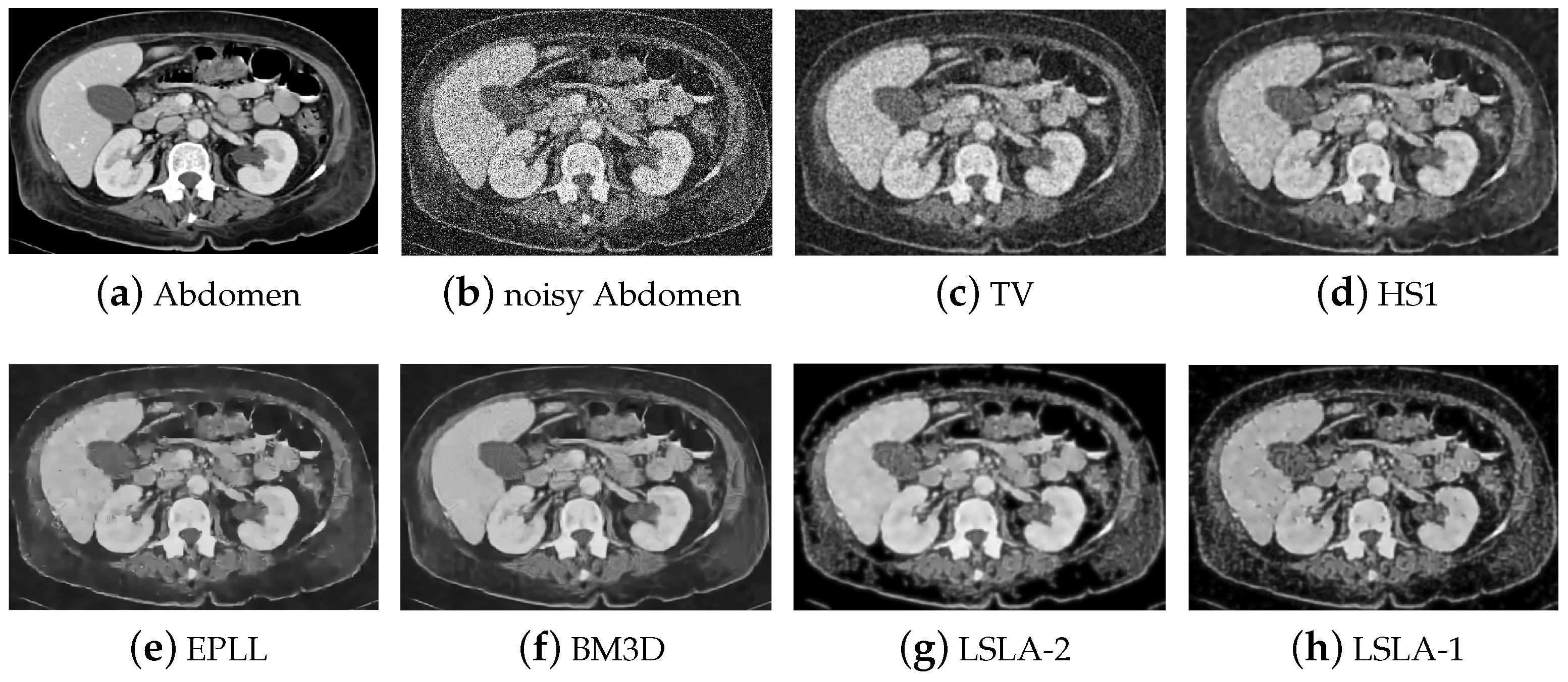
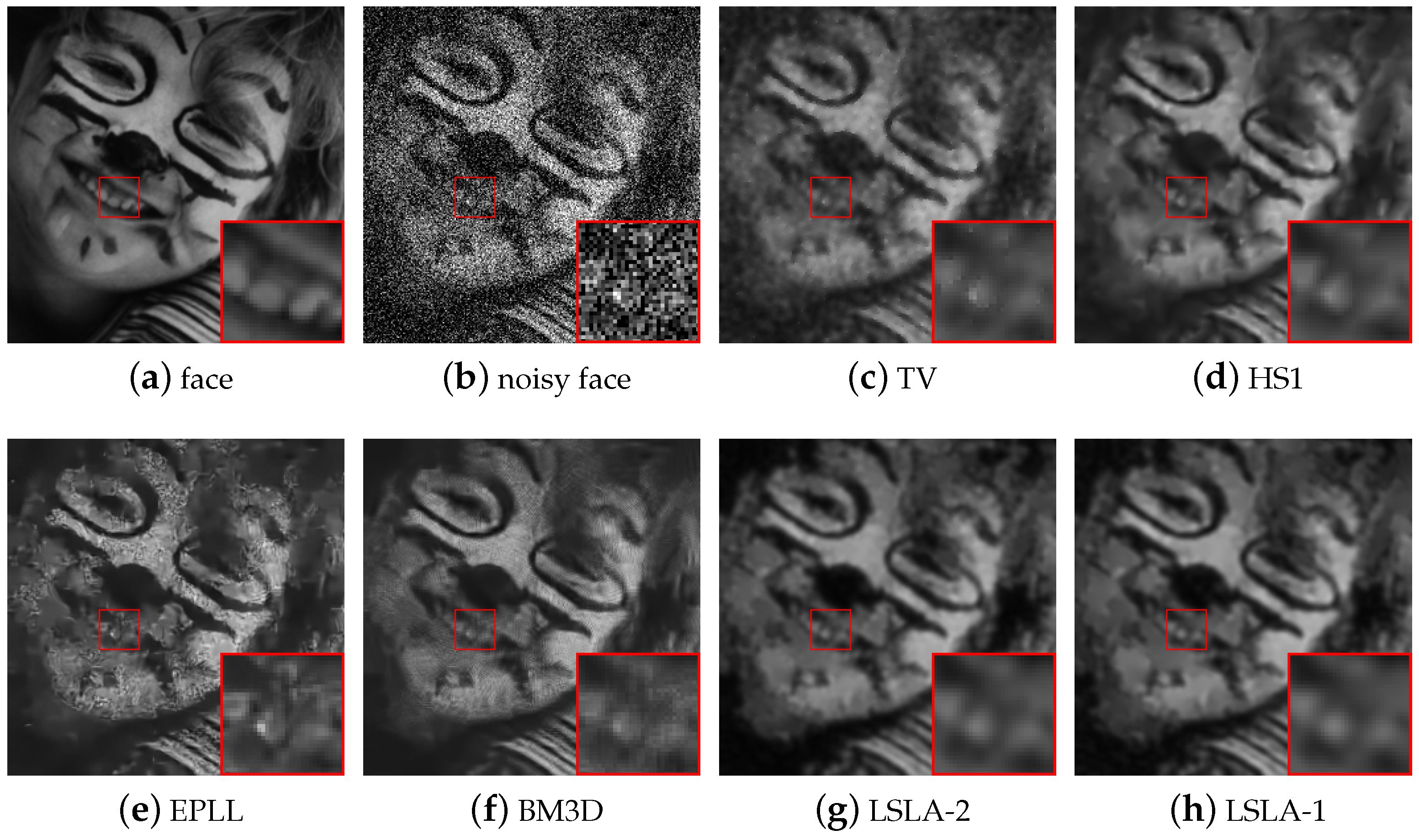
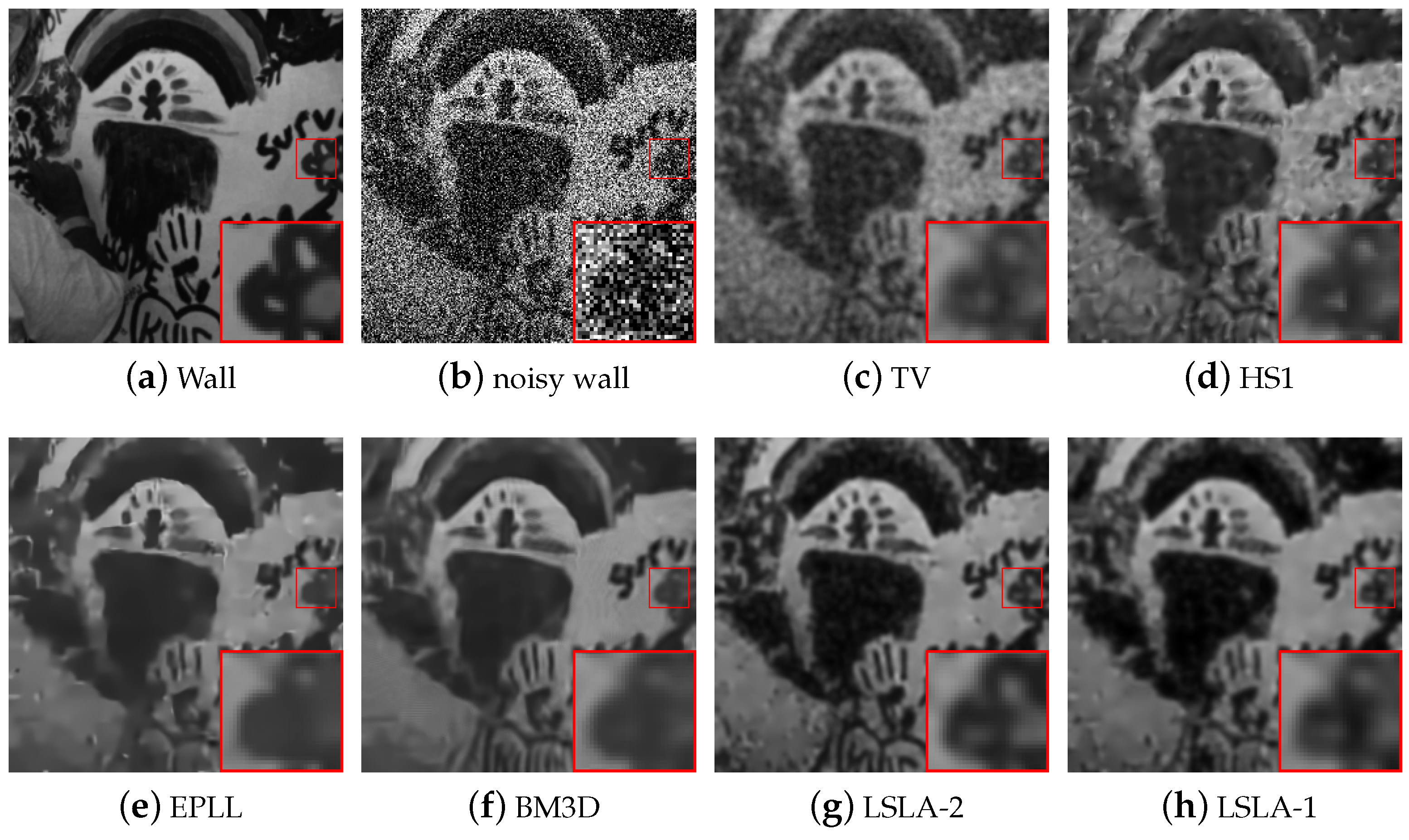
From Table 2, it is noted that our method has the best performance in PSNR in all cases and 11 out of 12 cases in SSIM with significant improvements. In terms of PSNR, our proposed method usually outperforms BM3D by around 1–2 dB. In addition, it is observed that our methods have improved SSIM by around 0.05 on Wall and Abdomen images. Overall, LSLA-1 and LSLA-2 produce the best results although Figure 1 shows that LSLA-1 has some dark peaks in the uniform regions (liver and kidney). To visually evaluate the performance, we show some visual results. Figure 1, Figure 2, Figure 3 and Figure 4 show some examples of the resulting images by different methods. Visually, BM3D results in very clean images, but many fine details are eliminated. To better show visual effects of the methods, we enlarge some local patches in Figure 3 and Figure 4. It is observed that indeed BM3D has an over smoothing effect and the major details are missing, whereas our methods keep such details. Moreover, it is observed that the brightness of different regions has changed in the images produced by BM3D, whereas our method shows similar brightness to the original ones. Our method shows similar results to TV and HS${}_1$ with more smoothing effects in the smooth region.

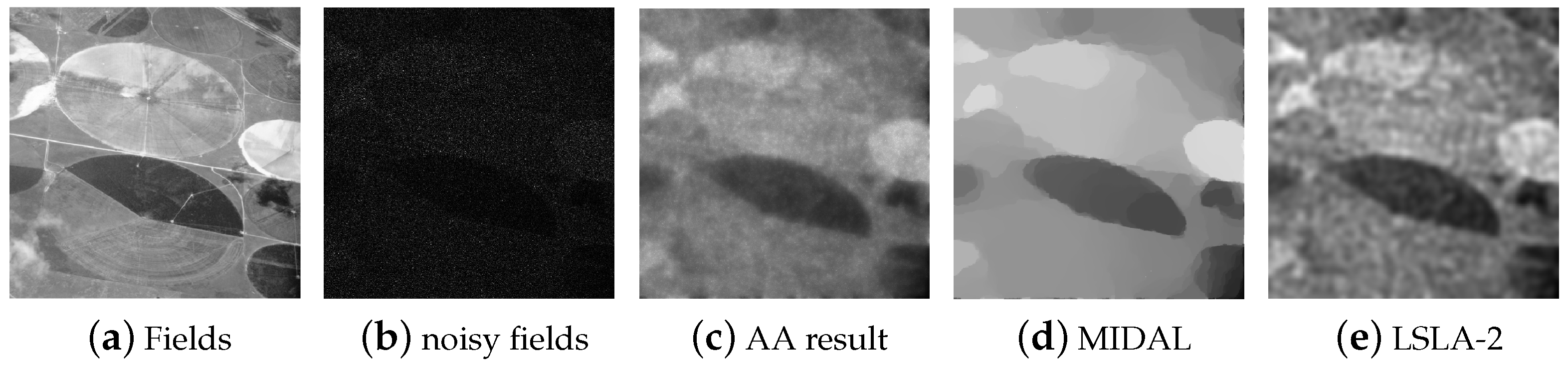
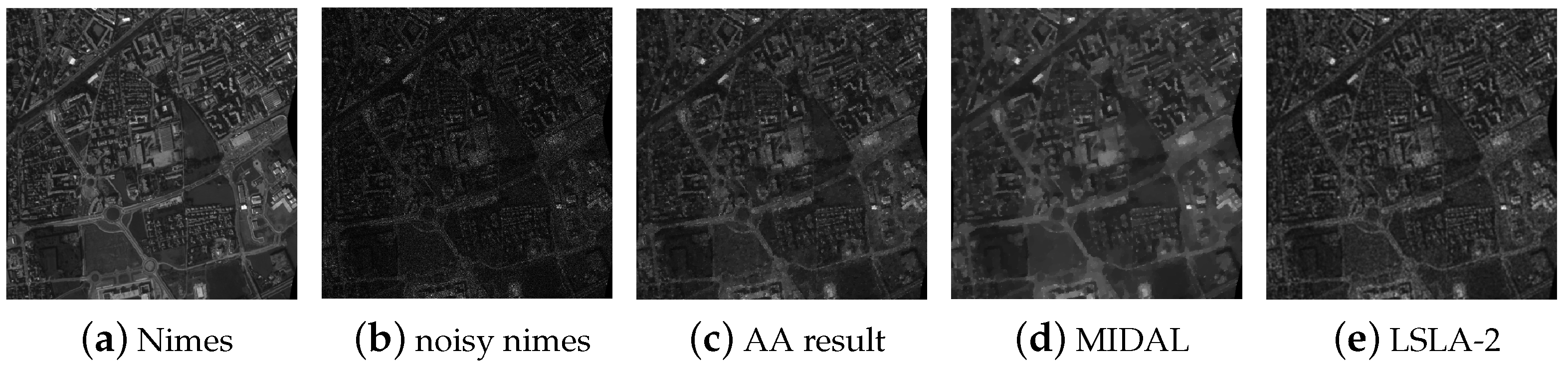
For multiplicative noise removal, it is seen that the proposed method has the best performance in all tests, except in one case when compared with MIDAL in SSIM. This observation, again, verifies that the proposed method is indeed effective for both additive and multiplicative noise removal. To visually evalute the results, we show some examples of the resulting images in Figure 5 and Figure 6. It is observed that the proposed method captures the edges well from the images, while MIDAL fails when the noise is strong. In the smooth regions, our method keeps the fine details such as the gradual change well, while MIDAL makes such gradual change difficult to distinguish. In addition, the intensities shown in the denoised images by our method appears to be much closer to the clean ones than AA and MIDAL because the contrast between the darkness and brightness is more like that in the clean images. Such observations have confirmed the effectiveness of the proposed method. At the same time, it can be seen that multiplicative noise is a much harder problem.

3.3. Parameter Sensitivity

For image denoising problem, it is hard to learn or theoretically analyze or the optimal parameters. To better investigate the performance of the proposed method, in this subsection, we present how the parameters affect the denoising performance. We have used the combination of parameters $\{{\lambda }_1,{\lambda }_2\}$ selected from the set $\{2,5,10,15,20\}\times \{0.01,0.05,0.1,0.2,0.3\}$. Without loss of generality, we test our method on two degraded images and report the results in Figure 7 where all combinations of parameters are used from the above set. It is seen that our method has comparablely high performance with a broad range of parameter values on both images, which implies the insensitivity of our method to the parameters. This observation indeed ensures the potential of our method in real world applications.

3.4. Time Comparison and Analysis

In this subsection, we test the time needed for the methods in comparison. Our simulations were performed in a MATLAB R2010b environment (MathWorks, Natick, Massachusetts, USA) on a Windows 7 operating system (Microsoft, Redmond, Washington, USA) with 2.60 GHz CPU and 4 GB RAM. Without loss of generality, we test the methods on images as given in Table 2, where average time costs are reported in

Table 4. Time comparison on Gaussian noise removal.

Algorithm	Time (s)
	Face	Kids	Wall	Abdomen
BM3D	1.0284	1.0336	1.1008	3.7333
HS1	16.9454	18.0842	17.5324	37.0296
EPLL	146.2443	78.3126	146.561	502.4728
TV	0.6696	0.6841	0.6538	1.3947
LSLA2	124.036	185.6624	122.9288	404.6401
LSLA1	169.4185	139.1726	178.3549	438.5715

for each image and method. It is observed that the proposed methods need more time than others except EPLL. Considering that our methods have superior performance in denoising results, such cost in time is fairly acceptable.

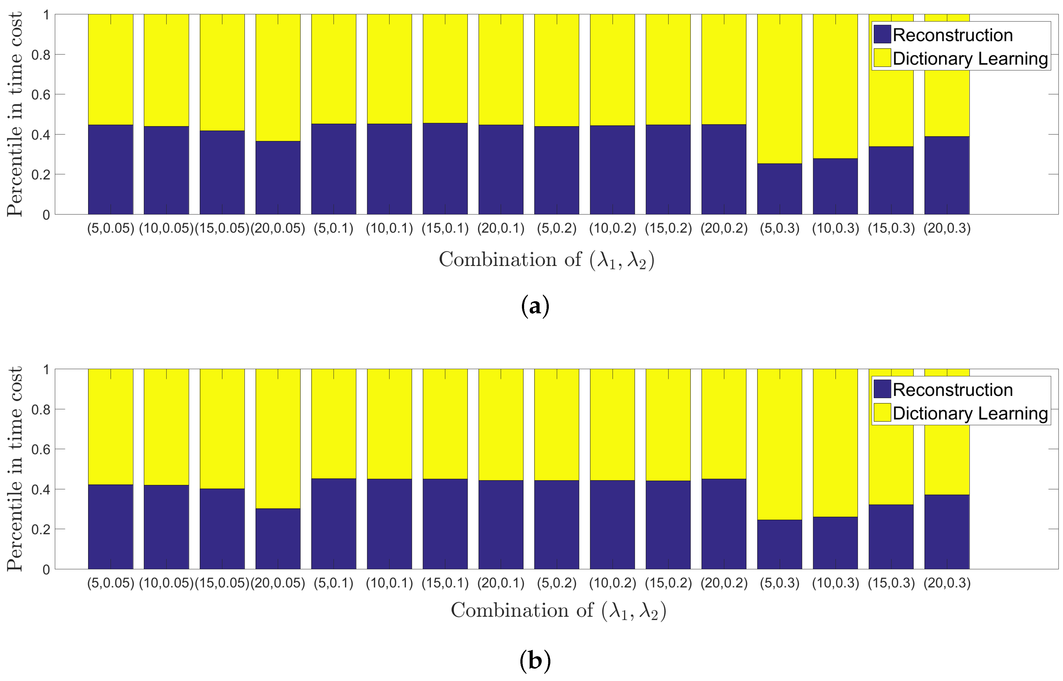
Moreover, we investigate the time cost for each stage of our algorithm. Without loss of generality, we report the results on Face and Kids images in Figure 8. It is seen that the second stage costs roughly 60% of the overall time on average. As the major step for time cost, it should be noted that this stage involves K-SVD, which generally is time-consuming. In this paper, we aim at proposing a new image denoising method and the way to speed up our method is not in the scope of our current work, which will be considered in the future.

3.5. Discussion

From the above experiments, it is seen that the proposed methods have superior performance to state-of-the-art algorithms both quantatively and visually. Quantatively, the proposed methods improve PSNR and SSIM significantly while visually they keep fine details of the images when other methods fail. Though the proposed method has slower speed than BM3D, TV, etc., it is noted that our method is comparable to some state-of-the-art algorithms such as EPLL, yet with superior performance. Hence, it is convincing to claim the stronger applicability of the proposed method to real world applications, such as hyperspectal image denoising, biomedical image denoising, or preprocessing of noisy image data for recognition, etc. Possible reasons for slower speed of the proposed method may be the need of matrix inverse operations and sparse coding, which generally have high cost. It is possible to speed up the proposed method with approximation techniques for matrix inverse or with more efficient sparse coding technique. This may be considered as a further line of research.

4. Conclusions

This paper presents an image denoising method that can be applied to both additive and multiplicative noise. The proposed method is designed to capture global structures and preserve local similarities simultaneously. This method produces promising results in terms of PSNR, SSIM and visual quality. The advantages of this novel method include the following: (1) for additive noise, our method outperforms or shows comparable results to TV , HS${}_1$ and BM3D methods either in terms of SSIM or PSNR; (2) for multiplicative noise, our method has performance superior to AA and MIDAL algorithms either in SSIM or PSNR; and (3) our method captures structures and keeps fine details well.

There are several future research directions. We are further exploring other optimization strategies for more effective convergence and further improvement. We are also considering transformation based method. Transformation and learning based model might potentially lead to more promising results.

References

- Jabarullah, B.M.; Saxena, S.; Babu, D.K. Survey on Noise Removal in Digital Images. IOSR J. Comput. Eng. 2012, 6, 45–51. [Google Scholar] [CrossRef]
- Chouzenoux, E.; Jezierska, A.; Pesquet, J.C.; Talbot, H. A Convex Approach for Image Restoration with Exact Poisson-Gaussian Likelihood. SIAM J. Imaging Sci. 2015, 8, 2662–2682. [Google Scholar] [CrossRef]
- Peng, C.; Cheng, J.; Cheng, Q. A Supervised Learning Model for High-Dimensional and Large-Scale Data. ACM Trans. Intell. Syst. Technol. 2017, 8, 30. [Google Scholar] [CrossRef]
- Peng, C.; Kang, Z.; Cheng, Q. Subspace Clustering via Variance Regularized Ridge Regression. In Proceedings of the IEEE Conference on Computer Vision and Pattern Recognition, Honolulu, HI, USA, 21–26 July 2017; pp. 682–691. [Google Scholar]
- Kang, Z.; Peng, C.; Cheng, Q. Kernel-driven similarity learning. Neurocomputing 2017, 267, 210–219. [Google Scholar] [CrossRef]
- Pham, D.L.; Xu, C.; Prince, J.L. Current methods in medical image segmentation. Annu. Rev. Biomed. Eng. 2000, 2, 315–337. [Google Scholar] [CrossRef] [PubMed]
- Buades, A.; Coll, B.; Morel, J.M. A Non-Local Algorithm for Image Denoising. In Proceedings of the IEEE Conference on Computer Vision and Pattern Recognition, San Diego, CA, USA, 20–25 June 2005; pp. 60–65. [Google Scholar]
- Chatterjee, P.; Milanfar, P. Is denoising dead? IEEE Trans. Image Process. 2010, 19, 895–911. [Google Scholar] [CrossRef] [PubMed]
- Rudin, L.I.; Osher, S.; Fatemi, E. Nonlinear total variation based noise removal algorithms. Phys. D Nonlinear Phenom. 1992, 60, 259–268. [Google Scholar] [CrossRef]
- Dabov, K.; Foi, A.; Katkovnik, V.; Egiazarian, K. Image Denoising by Sparse 3-D Transform-Domain Collaborative Filtering. IEEE Trans. Image Process. 2007, 16, 2080–2095. [Google Scholar] [CrossRef] [PubMed]
- Dong, W.; Shi, G.; Li, X. Nonlocal Image Restoration With Bilateral Variance Estimation: A Low-Rank Approach. IEEE Trans. Image Process. 2013, 22, 700–711. [Google Scholar] [CrossRef] [PubMed]
- Zuo, W.; Zhang, L.; Song, C.; Zhang, D. Texture Enhanced Image Denoising via Gradient Histogram Preservation. In Proceedings of the IEEE Conference on Computer Vision and Pattern Recognition, Portland, OR, USA, 23–28 June 2013; pp. 1203–1210. [Google Scholar]
- Fergus, R.; Singh, B.; Hertzmann, A.; Roweis, S.T.; Freeman, W.T. Removing camera shake from a single photograph. ACM Trans. Graph. 2006, 25, 787–794. [Google Scholar] [CrossRef]
- Han, Y.; Xu, C.; Baciu, G.; Li, M.; Islam, M.R. Cartoon and texture decomposition-based color transfer for fabric images. IEEE Trans. Multimed. 2017, 19, 80–92. [Google Scholar] [CrossRef]
- Lefkimmiatis, S.; Ward, J.P.; Unser, M. Hessian Schatten-Norm Regularization for Linear Inverse Problems. IEEE Trans. Image Process. 2013, 22, 1873–1888. [Google Scholar] [CrossRef] [PubMed]
- Harmeling, S. Image Denoising: Can Plain Neural Networks Compete with BM3D? In Proceedings of the IEEE Conference on Computer Vision and Pattern Recognition, Providence, RI, USA, 16–21 June 2012; pp. 2392–2399. [Google Scholar]
- Zoran, D.; Weiss, Y. From Learning Models of Natural Image Patches to Whole Image Restoration. In Proceedings of the IEEE International Conference on Computer Vision, Barcelona, Spain, 6–13 November 2011; pp. 479–486. [Google Scholar]
- Roth, S.; Black, M.J. Fields of Experts: A Framework for Learning Image Priors. Int. J. Comput. Vis. 2009, 82, 205. [Google Scholar] [CrossRef]
- Elad, M. Sparse and Redundant Representations: From Theory to Applications in Signal and Image Processing; Springer: Berlin/Heidelberg, Germany, 2010. [Google Scholar]
- Elad, M.; Aharon, M. Image denoising via sparse and redundant representations over learned dictionaries. IEEE Trans. Image Process. 2006, 15, 3736–3745. [Google Scholar] [CrossRef] [PubMed]
- Mairal, J.; Bach, F.; Ponce, J. Sparse modeling for image and vision processing. Found. Trends Comput. Graph. Vis. 2014, 8, 85–283. [Google Scholar] [CrossRef] [Green Version]
- Cai, S.; Weng, S.; Luo, B.; Hu, D.; Yu, S.; Xu, S. A Dictionary-Learning Algorithm based on Method of Optimal Directions and Approximate K-SVD. In Proceedings of the 35th Chinese Control Conference (CCC), Chengdu, China, 27–29 July 2016; pp. 6957–6961. [Google Scholar]
- Lin, Z.; Liu, R.; Su, Z. Linearized alternating direction method with adaptive penalty for low-rank representation. In Proceedings of the Advances in Neural Information Processing Systems, Granada, Spain, 12–14 December 2011; pp. 612–620. [Google Scholar]
- Yu, J.; Gao, X.; Tao, D.; Li, X.; Zhang, K. A unified learning framework for single image super-resolution. IEEE Trans. Neural Netw. Learn. Syst. 2014, 25, 780–792. [Google Scholar] [PubMed]
- Chen, S.S.; Donoho, D.L.; Saunders, M.A. Atomic Decomposition by Basis Pursuit; Society for Industrial and Applied Mathematics: Philadelphia, PA, USA, 1998. [Google Scholar]
- Cotter, S.F.; Rao, B.D. Sparse channel estimation via matching pursuit with application to equalization. IEEE Trans. Wirel. Commun. 2002, 50, 374–377. [Google Scholar] [CrossRef]
- Tropp, J.A.; Gilbert, A.C. Signal Recovery from Random Measurements via Orthogonal Matching Pursuit. IEEE Trans. Inf. Theory 2007, 53, 4655–4666. [Google Scholar] [CrossRef]
- Gorodnitsky, I.F.; Rao, B.D. Sparse signal reconstruction from limited data using FOCUSS: A re-weighted minimum norm algorithm. IEEE Trans. Signal Process. 2002, 45, 600–616. [Google Scholar] [CrossRef]
- Aharon, M.; Elad, M.; Bruckstein, A. K-SVD: An algorithm for designing overcomplete dictionaries for sparse representation. IEEE Trans. Signal Process. 2006, 54, 4311–4322. [Google Scholar] [CrossRef]
- Golub, G.H.; Van Loan, C.F. Matrix Computations; JHU Press: Baltimore, MD, USA, 2012; Volume 3. [Google Scholar]
- Rubinstein, R.; Zibulevsky, M.; Elad, M. Efficient Implementation of the K-SVD Algorithm using Batch Orthogonal Matching Pursuit. Cs Tech. 2008, 40, 1–15. [Google Scholar]
- Smith, L.N.; Elad, M. Improving dictionary learning: Multiple dictionary updates and coefficient reuse. IEEE Signal Process. Lett. 2013, 20, 79–82. [Google Scholar] [CrossRef]
- Lefkimmiatis, S.; Unser, M. Poisson image reconstruction with Hessian Schatten-norm regularization. IEEE Trans. Image Process. 2013, 22, 4314–4327. [Google Scholar] [CrossRef] [PubMed]
- Combettes, P.L.; Pesquet, J.C. Image restoration subject to a total variation constraint. IEEE Trans. Image Process. 2004, 13, 1213–1222. [Google Scholar] [CrossRef] [PubMed]
- Bioucas-Dias, J.M.; Figueiredo, M.A. Multiplicative noise removal using variable splitting and constrained optimization. IEEE Trans. Image Process. 2010, 19, 1720–1730. [Google Scholar] [CrossRef] [PubMed]
- Aubert, G.; Aujol, J.F. A variational approach to removing multiplicative noise. SIAM J. Appl. Math. 2008, 68, 925–946. [Google Scholar] [CrossRef]
Figure 1.
Results on the abdomeng image degraded by Gaussian noise of level = 0.1.
Figure 2.
Results on the kids image degraded by Gaussian noise of level = 0.07.
Figure 3.
Results on the face image degraded by Gaussian noise of level = 0.05.
Figure 4.
Results on the wall image degraded by Gaussian noise of level = 0.1.
Figure 5.
Results on the Fields image degraded by multiplicative noise of level L = 1.
Figure 6.
Results on the Nimes image degraded by multiplicative noise of level L = 4.
Figure 7.
Example of denoising performance changes with respect to parameters. From left to right are results on images of Face with Gaussian noise of level 0.05 and Kids with Gaussian noise of level 0.04.
Figure 8.
(a) Face image degraded by Gaussian noise of level 0.05; (b) Kids image degraded by Gaussian noise of level 0.04. Example of time cost on two stages using different combinations of parameters.