Efficient Superpixel-Guided Interactive Image Segmentation Based on Graph Theory

Abstract

Image segmentation is a challenging task in the field of image processing and computer vision. In order to obtain an accurate segmentation performance, user interaction is always used in practical image-segmentation applications. However, a good segmentation method should not rely on much prior information. In this paper, an efficient superpixel-guided interactive image-segmentation algorithm based on graph theory is proposed. In this algorithm, we first perform the initial segmentation by using the MeanShift algorithm, then a graph is built by taking the pre-segmented regions (superpixels) as nodes, and the maximum flow–minimum cut algorithm is applied to get the superpixel-level segmentation solution. In this process, each superpixel is represented by a color histogram, and the Bhattacharyya coefficient is chosen to calculate the similarity between any two adjacent superpixels. Considering the over-segmentation problem of the MeanShift algorithm, a narrow band is constructed along the contour of objects using a morphology operator. In order to further segment the pixels around edges accurately, a graph is created again for those pixels in the narrow band and, following the maximum flow–minimum cut algorithm, the final pixel-level segmentation is completed. Extensive experimental results show that the presented algorithm obtains much more accurate segmentation results with less user interaction and less running time than the widely used GraphCut algorithm, Lazy Snapping algorithm, GrabCut algorithm and a region merging algorithm based on maximum similarity (MSRM).

1. Introduction

Image segmentation, which aims to extract objects of interest from a complex background for object detection, tracking, recognition, scene analysis, etc., is one of the basic problems in image processing, and has been widely used in pattern recognition and computer vision [1,2,3,4,5,6,7]. Many image-segmentation algorithms have been proposed in recent years [5,6,7,8,9,10,11,12,13,14,15,16,17,18,19,20,21,22,23,24,25,26]. According to different image types, image segmentation can be divided into monochrome and color image segmentation. According to image representation, image segmentation can be divided into single scale and multi-scale approaches. According to the principle of operation, image segmentation can be divided into spatially blind and spatially guided methods. According to whether priori knowledge is provided, image segmentation can be divided into automatic and interactive segmentation. For natural images of various types and with complicated content, an interactive segmentation-based method is usually used, because its segmentation is more consistent with users’ subjective intentions [12,13,14,15,16,17,18,19,20]. GraphCut is one of the generally used interactive segmentation algorithms [13,14,15,16,17,18,19] due to its global optimization, strong numerical robustness, high execution efficiency, free topological structure of partitioned weighted graph, and N-D image-segmentation ability [13,14,15]. As a pre-segmentation solution, superpixel segmentation has been paid more attention and an abundance of superpixel segmentation algorithms have been proposed in recent years [7,21,22,23,24,25,26], such as watershed algorithms [21,22,23,24], MeanShift algorithm [25], turbopixels [26] etc. Superpixel algorithms group pixels into perceptually meaningful regions which can capture image redundancy and greatly reduce the complexity of subsequent image processing such as an object’s segmentation, detection, tracking and recognition tasks [6,7,18,20].

A good interactive image-segmentation method must perform accurate segmentation with minimal user interaction and less feedback time [17]. GraphCut is a representative interactive image-segmentation algorithm. It takes pixels as nodes to construct a weighted directed graph, and the maximum flow–minimum cut algorithm [14] is applied to obtain the global solution. Unfortunately, this algorithm only considers gray scale images, and hence the segmentation results are not good when the image content is complex. Moreover, when the pixel values in the foreground and background are closer in the gray scale, this algorithm usually requires users to provide a lot of interactive information to derive the ideal segmentation results. In addition, since pixels are used as nodes, the number of nodes in the graph model constructed by GraphCut algorithm would be huge when the image size is large, which also leads to the maximum flow–minimum cut algorithm taking a great deal of execution time. To overcome these shortcomings, Li et al. proposed the Lazy Snapping segmentation algorithm [18]. In this algorithm, the WaterShed algorithm [21] is first used to pre-segment images and a weighted directed graph is constructed by rendering the partitioned regions as nodes, and the maximum flow–minimum cut algorithm is then used to solve the graph partition problem. Finally, a manual adjustment scheme is adopted to make the segmentation results more accurate. This Lazy Snapping algorithm, however, has several major issues: (1) because the WaterShed algorithm only uses the gradient information of grayscale images, the over-segmentation is serious, and the number of regions of the pre-segmentation results is still large; (2) this algorithm uses the mean of color information to characterize each region, which is too simple to accurately represent the color distribution of each region; (3) in the modeling process, a K-means clustering algorithm is chosen, where the clustering performance is greatly affected by the initial conditions and disturbing factors; (4) this algorithm requires a lot of coarse-tuning and fine-tuning in the process of interaction, making the entire interactive process very complicated.

Compared with the WaterShed algorithm, the MeanShift segmentation algorithm [25] has been more widely studied and has a wider range of applications due to its excellent segmentation performance. The MeanShift algorithm makes full use of the color information, which suppresses over-segmentation effectively and the number of segmentation regions has been significantly reduced. Combining pre-segmentation by the MeanShift algorithm with color histogram representation for each region, Ning et al. proposed a region-merging algorithm based on maximum similarity (MSRM) [20]. By contrast with the maximum flow–minimum cut algorithm, a regional automatic merging mechanism is used to complete the color image segmentation for the MSRM algorithm. However, this algorithm only considers the similarity between adjacent regions and ignores the inter-relationship between each region with interaction information. In the process of region merging, the color histogram of each region needs to be made and simultaneously the similarity between adjacent regions needs to be calculated, and the whole space-time cost overhead is hence very expensive. In addition, the MSRM algorithm does not consider the over-segmentation problem introduced by the MeanShift algorithm, which leads to a large number of error segmentations around the edge of the targets.

To simplify the process of user interaction, Rother et al. proposed the GrabCut algorithm [19]. This algorithm establishes the initial foreground and background models, respectively, according to a rectangular area marked by users. Since in the rectangular area both foreground and background information are contained, the algorithm iteratively updates the foreground and background models through the iterative maximum flow–minimum cut scheme and iteration stops until the global energy solution is converged. In the initial step, only the background areas are determined accurately, so the final segmentation results for the GrabCut algorithm are affected by the initial background model.

In this paper, we present an efficient superpixel-guided interactive image-segmentation algorithm based on graph theory. Firstly, MeanShift algorithm is applied to pre-segment an image into regions (superpixels), and then the proposed algorithm constructs a weighted directed graph whose nodes are composed of the pre-partitioned regions. This model not only considers the correlation between adjacent superpixels, but also takes the relationship between each superpixel and the interaction information into account. Most importantly, we use the color histogram to represent each superpixel, which can accurately represent the regional color distribution. As with the MSRM segmentation algorithm, we choose Bhattacharyya coefficients to measure the similarity between superpixels, and the maximum flow–minimum cut algorithm is then performed to obtain the first-stage segmentation results. By considering the edge leakage problem caused by the MeanShift algorithm, the proposed algorithm creates a narrow band region by using the morphological operation at the boundary of targets based on the first-stage segmentation results. At the same time, the foreground and background regions are determined, and the corresponding foreground and background models are established by Gaussian mixed models (GMMs). Finally, a graph model is rebuilt again by considering pixels as nodes in the narrow band region and the final segmentation results are obtained by using the maximum flow–minimum cut algorithm. Through a large number of experiments, it is shown that the proposed algorithm achieves better segmentation results with less user interaction and execution time compared with the GraphCut, Lazy Snapping, GrabCut and MSRM algorithms.

The remainder of this paper is organized as follows: Section 2 summarizes the related work including the GraphCut, LazySnapping, GrabCut and MSRM algorithms. Section 3 introduces the motivation of the proposed algorithm and the detail is described in Section 4. Section 5 performs extensive experiments to verify the proposed algorithm. Section 6 concludes this paper.

2. Related Work

2.1. GraphCut Algorithm

The GraphCut algorithm [13] transforms the image-segmentation problem into graph-partition problem. It represents an image as a weighted directed graph G = (V, E, W), where V represents nodes of the graph corresponding to pixels in the image; E denotes the edges of the graph corresponding to connection between two adjacent nodes (usually for four or eight in the neighborhood); W is the weight of edges used to indicate the similarity of adjacent nodes. Before executing the maximum flow–minimum cut algorithm, users will be asked to first input the interaction information to mark the foreground (indicated by a set F) and the background (indicated by a set B); the other unmarked pixels are indicated by a set U and $V=F\cup B\cup U$. The foreground and background are modeled by the gray-scale histogram, and the two virtual nodes are then constructed as the source node (corresponding to the foreground model) and the sink node (corresponding to the background model). Among them, the weight is corresponding to the edges between any node in set V and the source/sink nodes, indicating the tendency that the corresponding node belongs to the foreground or the background. 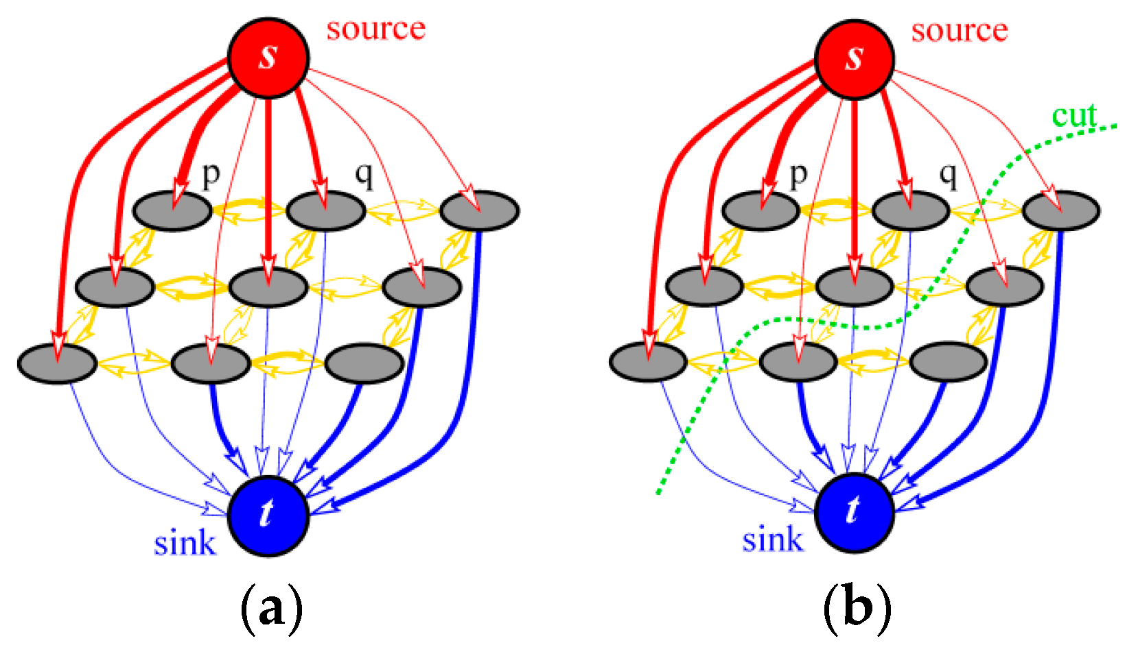Figure 1 shows a graph cut example for a 3 × 3 image, where Figure 1a is a directed graph composed of a pixels set V and two virtual nodes source and sink (denoted as s and t), and Figure 1b is an optimal cut solved by the maximum flow–minimum cut algorithm.

Figure 1. Graph cut example. (a) Graph; (b) cut.

The GraphCut algorithm solves the optimal segmentation problem by minimizing the following energy function,

$$E(\iota )=\lambda ·R(\iota )+B(\iota )$$

(1)

where $\iota$ is the segmented label value, 0 indicates the background and 1 indicates the foreground. $R(\iota )$ represents the area item, $B(\iota )$ represents the edge item, and the parameter $\lambda$ ($\lambda \ge 0$) is the balance factor between the region item and the edge item. $R(\iota )$ and $B(\iota )$ are defined as follows,

$$\{\begin{array}{l}R(\iota )={\displaystyle \sum _{i\in V}{R}_i({\iota }_i)}\\ B(\iota )={\displaystyle \sum _{\{i,j\}\in E}\left|{\iota }_i-{\iota }_j\right|·B_{\{i,j\}}}\end{array}$$

(2)

where, $R_i({\iota }_i)$ and $B_{\{i,j\}}$ are defined as follows,

$$\{\begin{array}{lll}{R}_i({\iota }_i=1)=K& R_i({\iota }_i=0)=0& \forall i\in F\\ R_i({\iota }_i=1)=0& R_i({\iota }_i=0)=K& \forall i\in B\\ R_i({\iota }_i=1)=-\ln \mathrm{Pr}(I_i|B)& R_i({\iota }_i=0)=-\ln \mathrm{Pr}(I_i|F)& \forall i\in U\end{array}$$

(3)

$$B_{\{i,j\}}=\exp \left(-\frac{{(I_i-I_j)}^2}{2{\sigma }^2}\right)·\frac{1}{dist(i,j)}$$

(4)

where, $K=1+\underset{i\in V}{\max }{\displaystyle \sum _{j: \{i,j\}\in N}B(i,j)}$, $N$ represents the neighborhood of pixels. $I_i$ represents the gray value of pixel $i$, $\mathrm{Pr}(I_i|F)$ represents the probability distribution value of $I_i$ in the histogram of the foreground $F$, and $\mathrm{Pr}(I_i|B)$ represents the probability distribution value of $I_i$ in the histogram of the background $B$. The parameter $\sigma$ is used to control the gray level difference between pixels $i$ and $j$, $dist(i,j)$ represents the spatial distance between pixels $i$ and $j$.

2.2. Lazy Snapping Algorithm

Since the GraphCut algorithm chooses pixels as nodes to construct a directed graph, the corresponding number of nodes is huge, which largely reduces the efficiency of this algorithm. In response to this problem, Li et al. proposed the Lazy Snapping algorithm [18]. By using the WaterShed algorithm [21], they pre-segment images and replace pixels in the GraphCut algorithm with processed regions as nodes. In addition, this algorithm used the color information instead of the gray information in the original GraphCut algorithm, which further improves the segmentation accuracy. Based on the region representation for graph nodes, Li et al. defined the following energy function,

$$E(\iota )={\displaystyle \sum _{i\in V}{E}_1({\iota }_i)}+\lambda {\displaystyle \sum _{(i,j)\in E}{E}_2({\iota }_i,{\iota }_j)}$$

(5)

where $E_1({\iota }_i)$ represents the likelihood energy and $E_2({\iota }_i,{\iota }_j)$ represents the prior energy. In the Lazy Snapping algorithm, Li et al. uses the mean color of each region (denoted as $C_i$) to represent the node, and the K-means algorithm was used to cluster the marked foreground pixels set $F$ and the background pixels set $B$. The corresponding clustering result centers are denoted as $K_n^F$ and $K_m^B$ respectively, where $n\in [1,\dots ,64]$, $m\in [1,\dots ,64]$.

Li et al. defined the likelihood energy and the priori energy as follows,

$$\{\begin{array}{lll}{E}_1({\iota }_i=1)=0& E_1({\iota }_i=0)=\infty & \forall i\in F\\ E_1({\iota }_i=1)=\infty & E_1({\iota }_i=0)=0& \forall i\in B\\ E_1({\iota }_i=1)=\frac{d_i^F}{d_i^F+d_i^B}& E_1({\iota }_i=0)=\frac{d_i^B}{d_i^F+d_i^B}& \forall i\in U\end{array}$$

(6)

$$E_2({\iota }_i,{\iota }_j)=\left|{\iota }_i-{\iota }_j\right|·g({\zeta }_{ij})$$

(7)

where, the minimal distance of region i to the foreground and background are calculated as $d_i^F=\underset{n}{\min }\Vert C_i-K_n^F\Vert$ and $d_i^B=\underset{m}{\min }\Vert C_i-K_m^B\Vert$ respectively, function $g(\xi )$ is defined as $g(\xi )=\frac{1}{\xi +1}$, and ${\zeta }_{ij}={\Vert C_i-C_j\Vert }^2$. It should be noted that although Equations (3) and (6) are exactly opposite, they can obtain the same segmentation results.

2.3. GrabCut Algorithm

In the process of interactive image segmentation, in order to further reduce user interaction Rother et al. proposed an efficient GrabCut segmentation algorithm [19]. The algorithm only needs users to draw a rectangle to cover objects to be segmented, where the outside part of the box is all the background and the inside part of the frame consists of the foreground and the background simultaneously. The GrabCut algorithm then applies the iterative maximum flow–minimum cut algorithm to extract objects automatically. The process of this algorithm is described as follows:

Step 1. Users complete the image marking by setting a rectangle.

Step 2. According to the users’ marking, the image is initially divided into two groups: pixels inside the rectangle are taken as the foreground (actually a mixture of foreground and background), and pixels outside the rectangle are taken as the background.

Step 3. A Gaussian mixed model (GMM) is created for the foreground and the background respectively, and each GMM has K Gaussian models.

Step 4. Dividing each pixel in the foreground into a Gaussian with the largest probability distribution value in the foreground Gaussian mixed model, and emphatically dividing each pixel in the background into a Gaussian with the largest probability distribution value in the background Gaussian mixed model.

Step 5. Updating each Gaussian distribution in the foreground and background respectively.

Step 6. Establishing a graph model by using all image pixels as nodes, the maximum flow–minimum cut algorithm is then implemented to complete the optimal graph partition of the current iteration.

Step 7. Repeating Steps 4–6, until the energy obtained in Step 6 no longer changes.

Compared with the GraphCut and Lazy Snapping algorithms, the interaction process of the GrabCut algorithm is simple. Because all the pixels outside the rectangle belong to background and their labels have been completely determined, in the iterative process it is only necessary to solve the optimal energy problem using the maximum flow–minimum cut algorithm for those pixels inside the rectangle.

2.4. Region Merging Algorithm Based on Maximum Similarity (MSRM)

Ning et al. proposed a region merging algorithm based on maximum similarity (MSRM) [20]. Firstly, this algorithm pre-segments a color image by the MeanShift algorithm [25], then chooses the Bhattacharyya coefficient to calculate the similarity between adjacent regions, and finally automatically completes the segmentation process through an iterative region-merging method. The MSRM algorithm quantizes the RGB color space of an image into $16\times 16\times 16=4096$ grids and then calculates the normalized histogram $H_i$ of each area. The similarity between two regions $i$ and $j$ measured by the Bhattacharyya coefficient is computed as follows:

$$\rho (i,j)={\displaystyle \sum _{k=1}^{4096}\sqrt{H_i(k)·H_j(k)}}$$

(8)

To complete the automatic image segmentation, Ning et al. defined the following region-merging rules: For any region $R$, let $Q$ be an adjacent region of $R$ and a set of all the adjacent regions of $Q$ is represented as ${\overline{S}}_Q={\{S_i^Q\}}_{i=1,2,\cdots }$, apparently the condition $R\in {\overline{S}}_Q$ is held. The similarity between $Q$ and its all adjacent regions is calculated by using Equation (8), and the ranking is performed from maximum to minimum. If $\rho (R,Q)=\underset{i=1,2,\cdots }{\max }\rho (S_i^Q,Q)$ is held, that is the similarity between $Q$ and $R$ is the largest, the region $Q$ should be merged into the region $R$. The merger algorithm is implemented in two steps: step one is to merge an unlabeled region in set $U$ with a background-labeled region $B$; and the other is the automatic merging between unlabeled regions in set $U$. The MSRM algorithm repeats the above two steps until iteration convergence when no new merging occurs.

3. Motivation

In the Lazy Snapping algorithm [18], a pre-segmentation scheme is implemented by using WaterShed algorithm [21], and pixels as nodes in original GraphCut algorithm [13] are replaced by the obtained pre-segmentation regions as new nodes, which effectively improve segmentation efficiency and performance. But this algorithm also has the following problems:

(1)

Each region in the Lazy Snapping algorithm is modeled by the mean of color in this region, which is not sufficient to describe each region effectively.

(2)

The K-Means algorithm is used in clustering of the marked seed points. This clustering algorithm is very sensitive to noise, singular points, number of clusters, initial clustering center etc. As a result, the clustering performance is often problematic.

(3)

The clustering process needs to set a larger number of centers. In the Lazy Snapping algorithm, the number of clusters for the foreground and the background is set to 64. This implies that users need to mark the foreground and background using at least 64 regions, which leads to much interactive work.

(4)

Because WaterShed segmentation algorithm is based on gradient information of grayscale image and ignore rich color information, serious over-segmentation happens and the number of segmentation regions is still abundant.

(5)

In order to get better segmentation results, Lazy Snapping algorithm uses a fine-tuning process to further improve the segmentation accuracy in the post-processing stage, but the consequence is that the entire interaction process is too cumbersome.

Compared with WaterShed algorithm, MeanShift algorithm [25] performs better, but with much less segmentation regions. Figure 2 illustrates the segmentation results obtained by using WaterShed algorithm and MeanShift algorithm respectively on a Flower image with size $500\times 351$ (175,500 pixels). WaterShed segmentation result contains 10,072 regions, while the MeanShift segmentation result contains only 1101 regions. In the proposed algorithm, we adopt the MeanShift algorithm as the pre-segmentation step to provide a good initialization for the subsequent high effective implementation of maximum flow–minimum cut algorithm.

Figure 2. Flower Image and Its Segmentation Results. (a) Flower Image; (b) WaterShed Segmentation Result; (c) MeanShift Segmentation Result.

On the other hand, compared with the GraphCut algorithm and the Lazy Snapping algorithm, the MSRM algorithm [20] improved a lot by incorporating an automatic merging mechanism. However, MSRM algorithm also has the following main problems:

(1)

This algorithm only considers the similarity between adjacent regions in the merging process without considering the relationship between each region and the foreground/background information marked by users. Generally speaking the MSRM algorithm does not make full use of the interactive information input by users, thereby slowing down the region-merging speed and weakening the segmentation accuracy greatly.

(2)

For each region, we need to calculate its color histogram before the merging algorithm is performed, and in the process of algorithm execution, it also needs to re-calculate the color histogram many times for each region after completing the region combination. In addition, in the region-merging process, it needs to calculate the similarity between each region with its adjacent regions according to Equation (8). In the whole segmentation process, this algorithm usually requires a large number of region merging, so its space-time overhead is very large.

(3)

The execution efficiency of MSRM algorithm has been seriously affected with increasing of the image size and the number of regions for those images with complex image content. Ning et al. has pointed out this problem in reference [20], so the application of this algorithm is limited to a certain extent.

(4)

Although MeanShift algorithm has excellent segmentation performance, the over-segmentation problem still exists in the segmentation results, and edge leak phenomenon occurs from time to time. But the MSRM algorithm does not do corresponding post-processing to resolve this problem.

By contrast with the GraphCut, Lazy Snapping and MSRM algorithms, the GrabCut algorithm [19] only needs to set a rectangular area for users to simplify the interaction process greatly. However, this algorithm also has several major problems:

(1)

Image content inside the rectangle marked by users contains both background and foreground information simultaneously, while the image content outside of the rectangle contains background information only. Although the algorithm establishes two models for foreground and background respectively at the same time, how accurate the establishment of the background model will be directly affects the final segmentation results.

(2)

When the size of an object is very large and almost occupies the whole space area in an image, or when the number of objects is large and is almost distributed in the whole image surface, the background area marked by users in the GrabCut algorithm is usually small. Due to insufficient background information, the established background model makes it difficult to represent the distribution of the background information in the whole image accurately. So the algorithm cannot obtain ideal segmentation results even after more iterations, and the whole process is very time-consuming.

(3)

This algorithm completes the modeling for the foreground through iterative online learning. Obviously, it is not effective compared with adopting the direct modeling scheme for the foreground. However, this modeling method for the GrabCut algorithm is determined by its interaction mode.

(4)

Since the number, area size and position distribution of targets in the image to be segmented directly determine the setting of the rectangular box, which cannot be changed by users in the interaction process, the flexibility of the interaction mode is poor. It seems that the execution efficiency and segmentation performance of the GrabCut algorithm are affected by the setting of the rectangular box on the image surface. However, from the above analysis, we can further find that the execution efficiency and segmentation performance of the GrabCut algorithm are essentially determined by the inherent characteristics of the image itself.

4. Proposed Algorithm

In this paper, we present an efficient superpixel-guided interactive image-segmentation algorithm based on graph theory. The proposed algorithm is completed in two stages. In the first stage, we first use the MeanShift algorithm to pre-segment the image to extract superpixels. The superpixels are then taken as nodes to construct a directed graph. Finally, we applied the maximum flow–minimum cut algorithm to complete superpixel-level based graph segmentation. In the second stage, in order to solve the boundary leakage problem caused by the MeanShift algorithm, the proposed algorithm creates a mask image, which is termed Trimap, using morphological erosion and expansion operations based on the first-stage segmentation results. This Trimap is composed of three parts: TrimapUnknown, TrimapForeground and TrimapBackground, respectively. The TrimapUnknown is a narrow band area containing both the background and foreground information. The TrimapForeground only contains foreground information, while the TrimapBackground only contains background information. Then we establish the corresponding foreground and background models for TrimapForeground and TrimapBackground respectively, and create a pixel-level graph model for the narrow band area. Finally the maximum flow–minimum cut algorithm is performed again to complete the pixel-level based image segmentation.

Because of the relatively large area of each region obtained in the pre-segmentation step using MeanShift, it is more effective to use the color histogram to represent each region than the color mean. Hence, as with the MSRM algorithm, the proposed algorithm also uses a color histogram to represent each superpixel, denoted as $H_i$ for superpixel $i$. For user-marked foreground $F$ and background $B$, a color histogram is also used to model them, which is denoted as $H^F$ and $H^B$ respectively. We still use the Bhattacharyya coefficient $\rho (i,j)$ to measure the similarity between adjacent superpixels $i$ and $j$, which is defined as Equation (8). In addition to measuring the similarity between superpixels, the similarity of each superpixel with respect to the foreground and the background is calculated as follows,

$$\{\begin{array}{l}\rho (i,F)={\displaystyle \sum _{k=1}^Z\sqrt{H_i(k)·H^F(k)}}\\ \rho (i,B)={\displaystyle \sum _{k=1}^Z\sqrt{H_i(k)·H^B(k)}}\end{array}$$

(9)

where $Z$ is the number of feature dimensions (size of the color histogram).

The above equations show that we not only consider the similarity between superpixels, but also consider the relationship between each superpixel and the interaction with the foreground and background, thus we define the following energy function,

$$E(\iota )={\displaystyle \sum _{i\in V}R({\iota }_i)}+{\displaystyle \sum _{(i,j)\in E}\left|{\iota }_i-{\iota }_j\right|·B({\iota }_i,{\iota }_j)}$$

(10)

where the first part is the regional term that measures the similarity between each superpixel and the interaction information with the foreground and background. The second part is the edge information that measures the similarity between adjacent superpixels. The definition of the regional term and the edge term is denoted as follows,

$$\{\begin{array}{lll}R({\iota }_i=1)=\hspace{1em}\mathsf{\Upsilon }& R({\iota }_i=0)=\hspace{1em}0& \forall i\in F\\ R({\iota }_i=1)=\hspace{1em}0& R({\iota }_i=0)=\hspace{1em}\mathsf{\Upsilon }& \forall i\in B\\ R({\iota }_i=1)=\rho (i,F)& R({\iota }_i=0)=\rho (i,B)& \forall i\in U\end{array}$$

(11)

$$B({\iota }_i,{\iota }_j)=\lambda ·\rho (i,j)$$

(12)

where, $\mathsf{\Upsilon }=1+\underset{i\in V}{\max }{\displaystyle \sum _{j: \{i,j\}\in N}\rho (i,j)}$, $N$ represents pixels neighborhood, and $\lambda$ is a balance control parameter.

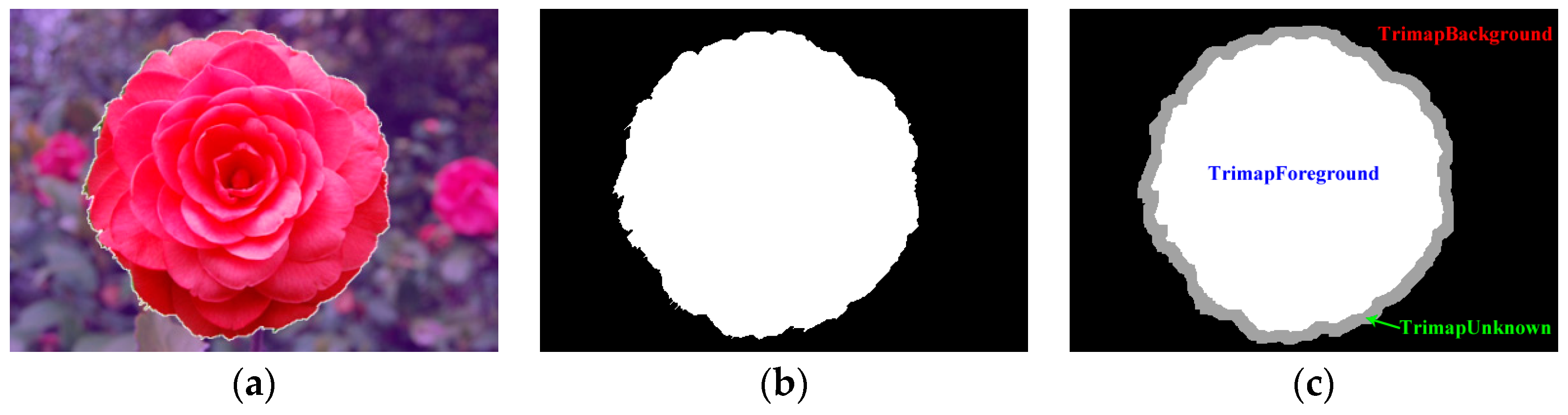
Figure 3 illustrates the segmentation result using the proposed method for the first stage on a rose image. As shown in Figure 3a, the edge of the target in the segmentation result is not smooth and there is some error segmentation due to the over-segmentation of the MeanShift algorithm. Therefore, based on the segmentation results of the first stage, we perform the segmentation process for the boundary region again. The corresponding binary image is denoted as $S$ and is shown in Figure 3b. In this process, we first morphologically erode the binary image $S$ to obtain a region $S_F=S\mathrm{\Theta }b$ which only contains objects and is described in white color (TrimapForeground) as shown in Figure 3c. Then, the morphological dilation operation is performed on the binary image $S$, and the difference between the dilation result and the erosion result is used as the narrow band region: $S_U=\left(S\oplus b\right)-\left(S\mathrm{\Theta }b\right)$, which contains both foreground and background and is represented in gray color (TrimapUnknown) in Figure 3c. The remaining area only contains the background information and can be expressed as $S_B=S-\left(S_U+S_F\right)$; we show it in black color (TrimapBackground) in Figure 3c. Here, we use the square structural element for the morphology process, where the element $b$ is in size $\left(2d+1\right)\times \left(2d+1\right)$ and $d$ is a positive integer. Finally, we obtain a triple mask image (Trimap) as in Figure 3c. We then use the Orchard–Bouman clustering algorithm [27] to create the corresponding Gaussian mixed model for the foreground and background, respectively. For each Gaussian mixed model the number of Gaussians is denoted as $K$. In addition, in order to solve the over-segmentation problem caused by the MeanShift algorithm and further improve the segmentation accuracy of the narrow band region, this paper takes pixels at the narrow band region as nodes to build a graph again and then applies the maximum flow–minimum cut algorithm to obtain the final segmentation results.

Figure 3. First stage segmentation result and ternary mask images. (a) Segmentation result in the first stage; (b) binary result; (c) Trimap.

The whole process of the second stage is basically similar to the GrabCut algorithm. But the difference is that the foreground region in the proposed algorithm is completely determined and is no longer an unknown region containing both foreground and background information. Therefore, the color model established in the first stage of the proposed algorithm does not need to be updated. Moreover, the maximum flow–minimum cut algorithm only needs to execute once to get the ideal segmentation results. The reason is that because the area size of the determined narrow band in the first stage is very small, the determined foreground and background regions almost contain all the foreground information and background information simultaneously. Therefore the foreground and background models established in the proposed algorithm are very accurate. In the second stage, we use the same energy function as Equation (10) in the first stage, but the corresponding two energy terms are redefined as follows,

$$\{\begin{array}{lll}R({\iota }_i=1)=\hspace{1em}\mathsf{\Upsilon }& R({\iota }_i=0)=\hspace{1em}0& \forall i\in \mathrm{TrimapForeground}\\ R({\iota }_i=1)=\hspace{1em}0& R({\iota }_i=0)=\hspace{1em}\mathsf{\Upsilon }& \forall i\in \mathrm{TrimapBackground}\\ R({\iota }_i=1)=D_B(i)& R({\iota }_i=0)=D_F(i)& \forall i\in \mathrm{TrimapUnknown}\end{array}$$

(13)

$$B({\iota }_i,{\iota }_j)=\frac{\lambda }{dist(i,j)}\exp \left(-\frac{{\Vert I_i-I_j\Vert }^2}{2{\sigma }^2}\right)$$

(14)

where, $I_i$ represents the color information of pixel $i$ and $\mathsf{\Upsilon }=1+\underset{i\in V}{\max }{\displaystyle \sum _{j: \{i,j\}\in N}B({\iota }_i,{\iota }_j)}$. In the process of building a graph model, we use 8 neighborhoods, and since $\lambda \ge B({\iota }_i,{\iota }_j)$ is satisfied, we set $K=8\lambda +1$. $D_x\left(i\right)$ (variable $x$ satisfies $x\in \left\{F,B\right\}$) is the distribution of the $i$th pixel in the foreground or background model following the Gaussian mixed model, which is calculated as:

$$D_x\left(i\right)=-\log {\displaystyle \sum _{k=1}^K{\pi }_k^x\frac{1}{\sqrt{\det {\sum }_k^x}}\exp \left(-\frac{1}{2}{\left[I_i-{\mu }_k^x\right]}^{\mathrm{T}}{\left({\sum }_k^x\right)}^{-1}\left[I_i-{\mu }_k^x\right]\right)}$$

(15)

where, ${\pi }_k^x$ denotes the weight of the $k$th Gaussian distribution in the Gaussian mixed model of the foreground or background, ${\mu }_k^x$ and ${\sum }_k^x$ denote the mean and covariance matrix of the $k$th Gaussian distribution in the foreground or background model, and $\det {\sum }_k^x$ denotes the determinant of covariance of matrix ${\sum }_k^x$.

From the above description of the proposed algorithm, we can see that the proposed algorithm only requires a small amount of interaction information and can obtain ideal segmentation results in a relatively short period of time. As shown in Figure 2, before executing the GraphCut algorithm, users are asked to input interactive information in Figure 2a. However, each pixel needs to be determined. As for Figure 2b, although it is area-based segmentation, it is still difficult for users to decide which areas should be marked before performing the Lazy Snapping algorithm, while in Figure 2c, the large area size and small number of areas provides guidance for user interaction and simplifies the interaction process. In addition, compared with the MSRM algorithm, the proposed algorithm not only takes the similarity between regions into account, but also the similarity between each region and the foreground/background information. Furthermore, the proposed algorithm could accurately determine the foreground and background regions after the first stage segmentation process. Compared with the GrabCut algorithm, the established background model is more accurate and, most importantly, the foreground model is also established at the same time. For those images that contain only one large size object or a large number of objects almost distributed over the entire image, it is difficult to obtain ideal segmentation results using the GrabCut algorithm even if the maximum flow–minimum cut algorithm is applied more times.

5. Experimental Results

We performed the experiment on some public datasets. Figure 4 shows three testing images and Table 1 shows some basic information of the testing images, including the image size, the total number of pixels, the number of superpixels segmented using the WaterShed [21] and MeanShift [25] algorithms, respectively. As can be clearly seen from the table, compared with the number of pixels, the number of superpixels processed by the pre-segmentation techniques has been greatly reduced, where we can see that the MeanShift algorithm is more effective than the WaterShed algorithm. In the experiment, the parameters of our method were set as follows: the size of the color histogram was set as $Z=4096$, the balance control parameter in the graph model was set as $\lambda =1.0$, the size of the square structural element in the morphology process was set as $b=2$, and the number of Gaussians of GMMs in the foreground and background models was set as $K=5$. All the parameter values were set by following exhaustive experiments.

Figure 4. Test images. (a) Flower; (b) person; (c) animal.

Table 1. Number of pixels and superpixels of three test images.

Test Image	Image Size	# of Pixels	# of Superpixels for WaterShed	# of Superpixels for MeanShift
Flower	500 × 351	175,500	10,072	1101
Person	399 × 384	153,216	9632	560
Animal	335 × 295	98,825	7131	196

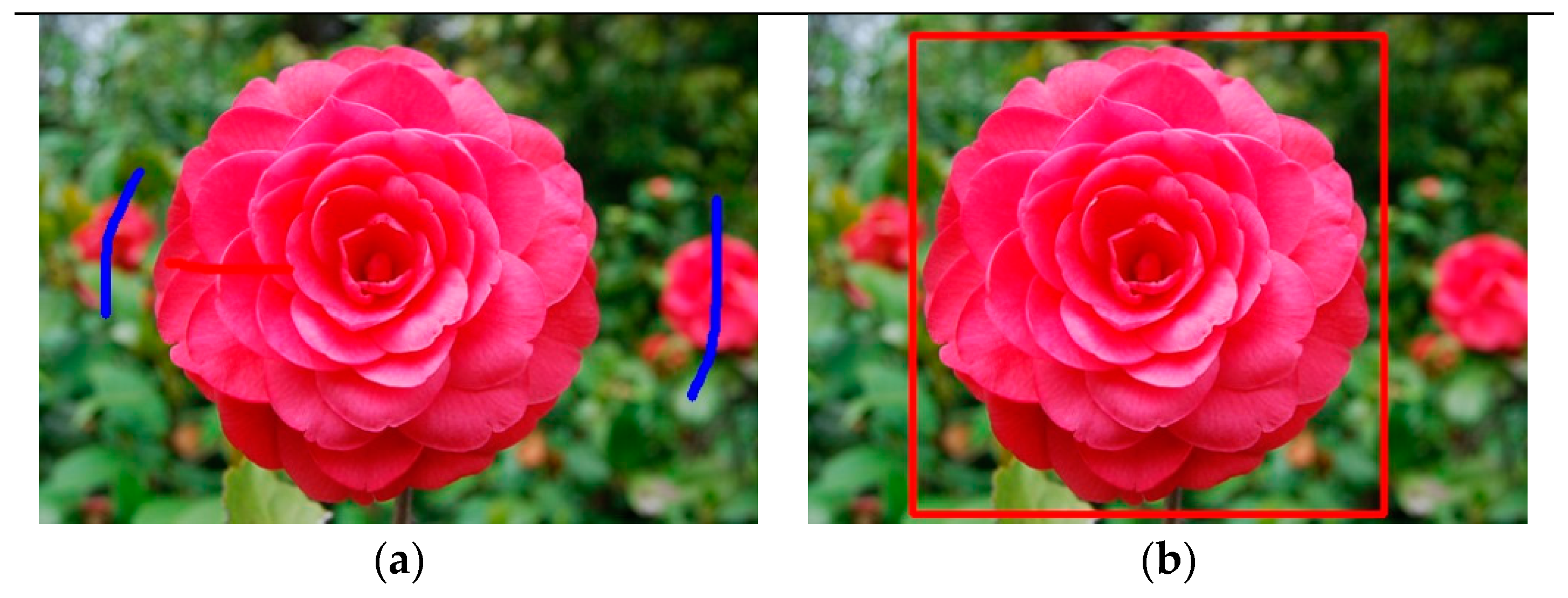
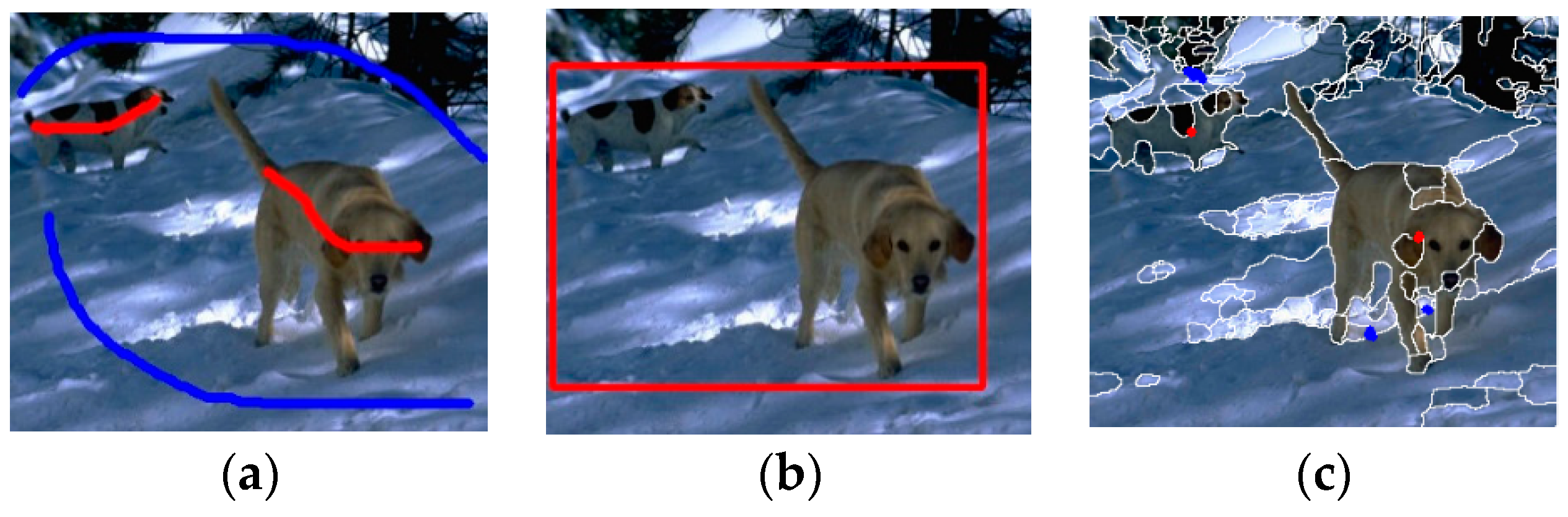
Figure 5 shows the interaction information marked by users for the flower image. For the sake of fairness, the GraphCut [13], Lazy Snapping [18] and MSRM [20] algorithms and the proposed algorithm use the same interaction information, as shown in Figure 5a. The red strokes mark foreground information and the blue strokes mark background information. Because the GrabCut algorithm [19] completes the user interaction by setting a rectangular area, different from the above four algorithms, we only need to mark a red box as shown in Figure 5b. All pixels outside of the red box belong to the background, the others containing both the foreground and background are segmented iteratively by the maximum flow–minimum cut algorithm. Figure 6 illustrates the corresponding segmentation results of each algorithm, where the first row is the original image-segmentation results and the second row is the corresponding binary images. From the experimental results, we can see that the GraphCut and Lazy Snapping algorithms have a large number of misclassifications. Although the GrabCut algorithm is good at boundary processing, there are some misclassifications inside the target, which can be seen from the corresponding binary image. The segmentation result of the MSRM algorithm is ideal inside the foreground and background, but over-segmentation is serious around the edge of the target, which is similar to the segmentation result in the first stage of the proposed algorithm, as shown in Figure 3a. After the second pixel-level based segmentation for the narrow band, the proposed algorithm effectively solves the edge leakage problem, resulting in a good segmentation result, as shown in Figure 6e below.

Figure 5. User interaction for the flower image. (a) Interaction of GraphCut, Lazy Snapping, MSRM and proposed algorithms; (b) interaction of GrabCut.

Figure 6. Segmentation results for the flower image. (a) GraphCut; (b) Lazy Snapping; (c) GrabCut; (d) MSRM; (e) proposed algorithm.

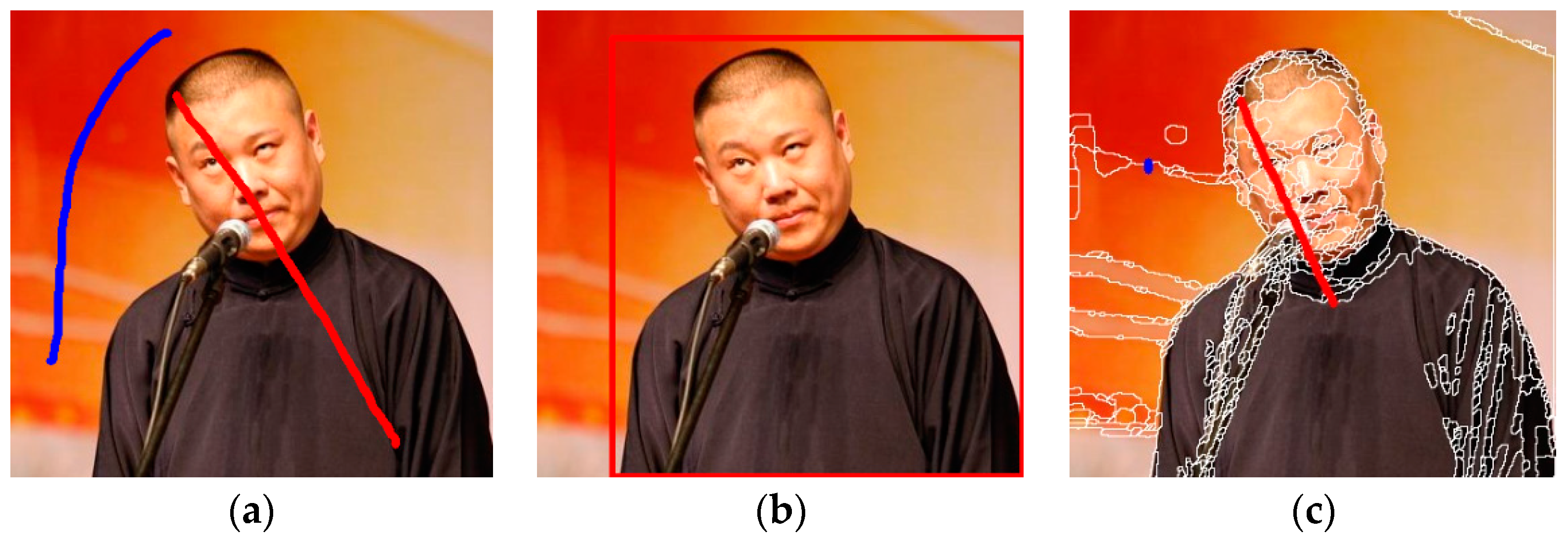
Figure 7 illustrates the interaction information marked by users for the person image. Since the number of regions partitioned by the WaterShed algorithm is still large and the area size is generally small, no guide information can be provided to users in the interaction process. Therefore, in this experiment, the GraphCut and Lazy Snapping algorithms use the same interaction information. Because the MSRM algorithm and our algorithm use the same pre-segmentation MeanShift algorithm, the two algorithms use the same interaction information. As shown in Figure 7c, only a few marks are needed to determine a large amount of background and foreground information. The corresponding segmentation results are shown in Figure 8. Because of the fewer background area markers, as shown in Figure 7a, a large number of misclassifications in the GraphCut and Lazy Snapping algorithms occur. The main reason is that because users find it hard to make accurate interactive marking without guidance, this problem becomes more prominent when the image content is complex. As with the flower image, the segmentation result of GrabCut algorithm is also acceptable. This is because the background information outside the rectangle area can fully represent the background distribution of the image, and the established background model is relative accurate. However, only having the accurate background model is not enough, and we can see some misclassifications inside the target. Furthermore, because the MeanShift algorithm has the problem of edge leakage in the segmentation process, the misclassification of the segmentation result of the MSRM algorithm is still serious at the target edge, as shown in Figure 8d. In contrast, the segmentation result of the proposed algorithm performs much better than the others in terms of segmentation accuracy, especially in the target boundary areas, as shown in Figure 8e.

Figure 7. User interaction for the person image. (a) Interaction of GraphCut and Lazy Snapping; (b) interaction of GrabCut; (c) interaction of MSRM and proposed algorithm.

Figure 8. Segmentation results for the person image. (a) GraphCut; (b) Lazy Snapping; (c) GrabCut; (d) MSRM; (e) proposed algorithm.

In addition, Figure 9 shows the user interaction for the animal image and the segmentation results are shown in Figure 10. From the segmentation results, we can find that the segmentation results of the GraphCut and Lazy Snapping algorithms are not perfect even when a lot of marker information is used. For example, it is difficult for users to mark the narrow tail region, which leads to false segmentation of this region. For the GrabCut algorithm, because the two targets (dogs) are scattered in the image, the marked background information is not enough to represent the background distribution effectively, and a large amount of background information is contained in the rectangular area. Thus, it is difficult for the GrabCut algorithm to learn the background model accurately. Although the MSRM algorithm has the same initial conditions with the proposed algorithm, it can be seen from Figure 9c that the segmentation results by using the MSRM algorithm have a large number of errors. The main reason is that the MSRM algorithm only considers the similarity among regions and does not fully consider the relationship between regions and the interaction information marked by users. Although the GraphCut, Lazy Snapping, GrabCut and MSRM algorithms can improve segmentation accuracy by adding more markers, the interaction process is more complicated. However, the proposed method achieves very promising segmentation results under the same user interaction or less marking conditions, which is more effective in practical applications.

Figure 9. User interaction for the animal image. (a) Interaction of GraphCut and Lazy Snapping; (b) interaction of GrabCut; (c) interaction of MSRM and proposed algorithm.

Figure 10. Segmentation results for the animal image. (a) GraphCut; (b) Lazy Snapping; (c) GrabCut; (d) MSRM; (e) proposed algorithm.

Table 2 compares the running time of the five algorithms. As can be seen from the table, the proposed algorithm has almost the same efficiency in terms of running time with the GraphCut and Lazy Snapping algorithms. Although the segmentation performance of the GrabCut algorithm is relatively good, it is not efficient to use in real-time applications. The execution efficiency of the MSRM algorithm is mainly determined by the number of partitioned regions, which is also not robust for practical implementation. For our proposed algorithm, the high efficiency of the maximum flow–minimum cut algorithm and its property of being less sensitive to the number of regions makes it efficient and useful for real-time segmentation.

Table 2. Running time comparison (ms).

Testing Images	GraphCut	Lazy Snapping	GrabCut	MSRM	Proposed Algorithm
Flower	579	422	9766	4797	750
Person	703	407	13,954	2500	578
Animal	281	265	3109	516	343

In order to further compare our proposed algorithm with the other four algorithms, we perform a detailed experiment on the Microsoft GrabCut image dataset [19], which is composed of 30 images provided with ground truth. Some testing images and the corresponding ground truth are shown in Figure 11. In this experiment, we evaluated the segmentation performance using the misclassification error (ME) [5], Rand index (RI) [28] and boundary recall (BR) [26]. ME is defined as follows,

$$ME=1-\frac{\left|B_G\cap B_S\right|+\left|F_G\cap F_S\right|}{\left|B_G\right|+\left|F_G\right|}$$

(16)

where $B_G$ and $F_G$ denote the background and foreground pixels of the ground truth ($G$), $B_S$ and $F_S$ denote the background and foreground pixels of the segmentation result ($S$), and $|•|$ is the cardinality of the set. The ME measures the percentage of wrongly assigned pixels, which ranges from zero for no error and one for completely wrong.

Figure 11. Partial test images and ground truth of the GrabCut image dataset.

RI computes the ratio of the number of pixel-pairs sharing the same label relationship between the segmentation result ($S$) and the ground truth ($G$). The definition of RI is described as follows,

$$RI=\frac{1}{\left({}_2^N\right)}{\displaystyle \sum _{i,j,i<j}\left[\mathrm{I}\left(l_i^S=l_j^S\right)·\mathrm{I}\left(l_i^G=l_j^G\right)+\mathrm{I}\left(l_i^S\ne l_j^S\right)·\mathrm{I}\left(l_i^G\ne l_j^G\right)\right]}$$

(17)

where $N$ denotes the total number of pixels, $\mathrm{I}\left(·\right)$ is a binary function with $\mathrm{I}\left(1\right)=1$ and $\mathrm{I}\left(0\right)=1$. The RI takes values in the range [0, 1], where a score of zero indicates the labelling of the test segmentation is totally opposite to the ground truth and 1 indicates that they are the same on every pixel pair.

BR measures the percentage of the ground truth boundaries recovered by the segmentation boundaries and is defined as follows,

$$BR=\frac{{\displaystyle {\sum }_{p\in G_b}\mathrm{I}\left({\min }_{q\in S_b}\Vert p-q\Vert <2\right)}}{\left|G_b\right|}$$

(18)

where $S_b$ and $G_b$ denote the union sets of segmentation boundaries and ground truth boundaries, respectively.

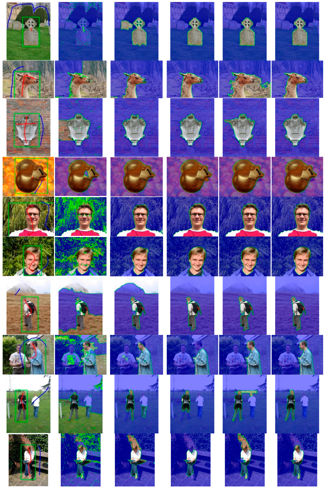
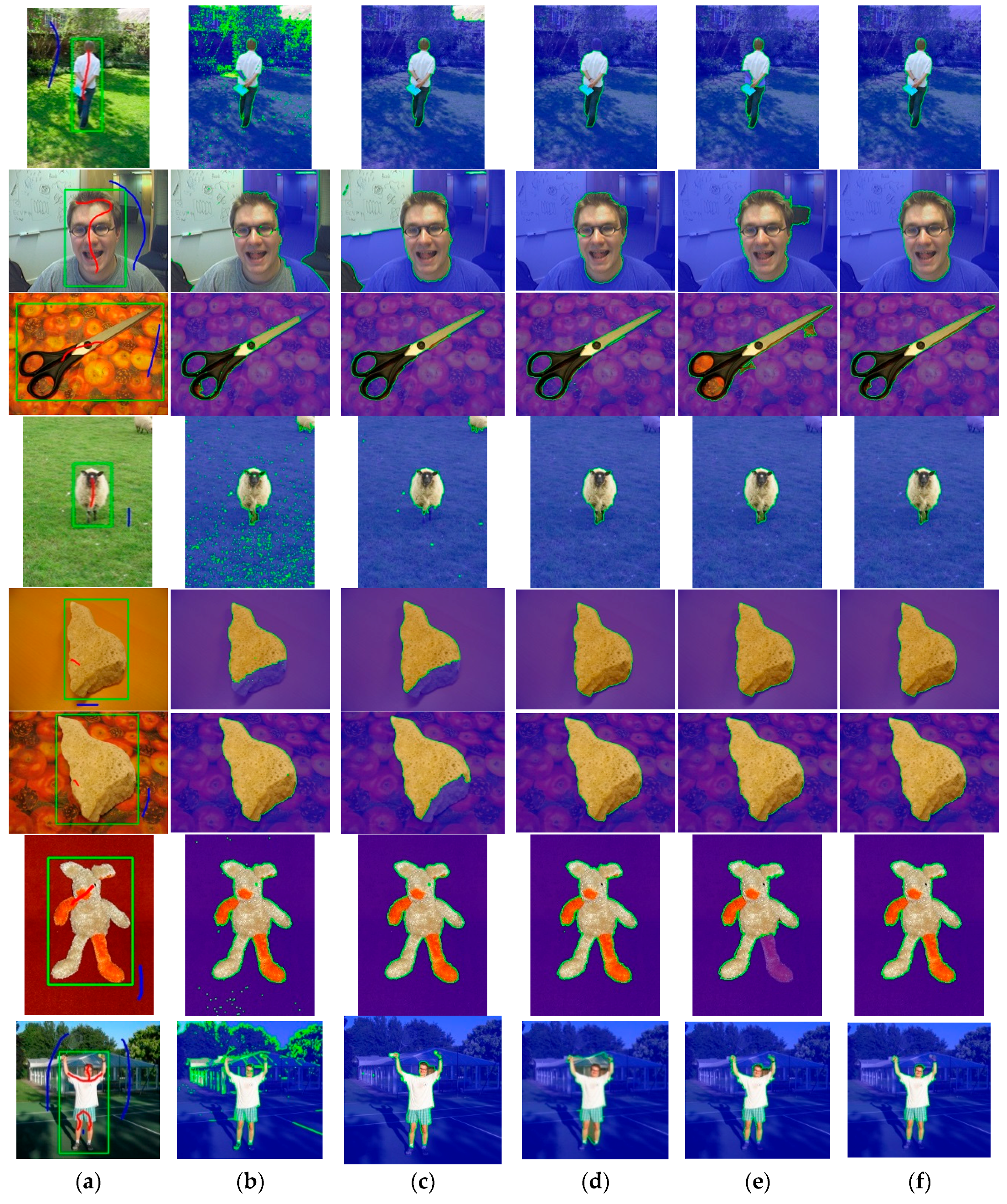
The segmentation results are illustrated in Figure 12, Table 3, Table 4 and Table 5. Similarly, the GraphCut, Lazy Snapping algorithm and MSRM algorithms and the proposed algorithm use the same interaction information, as shown in Figure 12a, where the red strokes mark the foreground and the blue strokes mark the background. The green rectangular box is used for the GrabCut algorithm as also shown in Figure 12a. From the segmentation results, we find that the proposed algorithm obtains the overall best segmentation performance in ME, RI and BR measures.

Figure 12. Segmentation results on the GrabCut image dataset for different algorithms. (a) Interaction markers; (b) GraphCut; (c) Lazy Snapping; (d) GrabCut; (e) MSRM; (f) proposed algorithm.

Table 3. Misclassification error (ME) comparison.

Images	GraphCut	LazySnapping	GrabCut	MSRM	Proposed Algorithm
banana1	0.6030	0.0142	0.2942	0.0163	0.0097
banana2	0.1718	0.0183	0.0087	0.0199	0.0102
banana3	0.1513	0.0226	0.0148	0.0197	0.0146
book	0.4628	0.0239	0.0218	0.0207	0.0218
bool	0.1146	0.0397	0.1708	0.0242	0.0105
bush	0.2149	0.1242	0.0188	0.0194	0.0121
ceramic	0.2142	0.0107	0.0083	0.0114	0.0072
cross	0.0112	0.0121	0.2736	0.0151	0.0129
doll	0.2654	0.1462	0.0121	0.0069	0.0050
elefant	0.0891	0.0361	0.0738	0.0366	0.0345
flower	0.0412	0.0073	0.0038	0.0061	0.0033
fullmoon	0.0014	0.0014	0.0034	0.0039	0.0014
grave	0.1192	0.0398	0.0068	0.0076	0.0059
llama	0.4716	0.0295	0.009	0.2397	0.0127
memorial	0.0912	0.0138	0.0159	0.0236	0.0145
music	0.0157	0.0090	0.0111	0.0082	0.0062
person1	0.1519	0.0088	0.0087	0.0072	0.0053
person2	0.1797	0.0124	0.0293	0.0068	0.0057
person3	0.4749	0.2164	0.0048	0.0080	0.0038
person4	0.2364	0.0316	0.0421	0.0144	0.0129
person5	0.4488	0.0307	0.0162	0.0236	0.0046
person6	0.0807	0.0628	0.0273	0.0597	0.0090
person7	0.0593	0.0263	0.0071	0.0103	0.0024
person8	0.5804	0.2487	0.0127	0.0232	0.0086
scissors	0.0237	0.0168	0.0174	0.0491	0.0129
sheep	0.0260	0.0157	0.0040	0.0048	0.0035
stone1	0.0509	0.0442	0.0024	0.0033	0.0020
stone2	0.0037	0.0479	0.0038	0.0052	0.0028
teddy	0.0065	0.0081	0.0070	0.0431	0.0095
tennis	0.0658	0.0131	0.0426	0.0150	0.0100
Avg. ME	0.1809	0.0444	0.0391	0.0251	0.0092

Table 4. Rand index (RI) comparison.

Images	GraphCut	LazySnapping	GrabCut	MSRM	Proposed Algorithm
banana1	0.5212	0.9720	0.5847	0.9679	0.9807
banana2	0.7154	0.9641	0.9828	0.9610	0.9799
banana3	0.7431	0.9558	0.9708	0.9613	0.9712
book	0.5028	0.9534	0.9573	0.9594	0.9573
bool	0.7971	0.9238	0.7167	0.9527	0.9791
bush	0.6625	0.7824	0.9630	0.9620	0.9761
ceramic	0.6633	0.9789	0.9836	0.9775	0.9857
cross	0.9779	0.9762	0.6025	0.9703	0.9745
doll	0.6100	0.7504	0.9761	0.9862	0.9900
elefant	0.8377	0.9304	0.8632	0.9296	0.9334
flower	0.9209	0.9855	0.9924	0.9878	0.9934
fullmoon	0.9973	0.9972	0.9931	0.9922	0.9972
grave	0.7900	0.9236	0.9865	0.9849	0.9883
llama	0.5016	0.9428	0.9823	0.6355	0.9750
memorial	0.8342	0.9727	0.9687	0.9539	0.9714
music	0.9692	0.9821	0.9780	0.9838	0.9877
person1	0.7424	0.9826	0.9828	0.9856	0.9895
person2	0.7052	0.9755	0.9432	0.9865	0.9887
person3	0.5013	0.6608	0.9904	0.9842	0.9924
person4	0.6389	0.9388	0.9193	0.9716	0.9744
person5	0.5052	0.9404	0.9682	0.9539	0.9909
person6	0.8517	0.8823	0.9468	0.8878	0.9821
person7	0.8885	0.9488	0.9858	0.9796	0.9952
person8	0.5129	0.6263	0.9748	0.9547	0.9829
scissors	0.9538	0.9670	0.9658	0.9066	0.9746
sheep	0.9493	0.9691	0.9920	0.9904	0.9930
stone1	0.9033	0.9154	0.9953	0.9934	0.9960
stone2	0.9927	0.9088	0.9924	0.9897	0.9944
teddy	0.9872	0.9839	0.9862	0.9176	0.9811
tennis	0.8771	0.9741	0.9185	0.9705	0.9801
Avg. RI	0.7685	0.9222	0.9354	0.9546	0.9819

Table 5. Boundary recall (BR) comparison.

Images	GraphCut	LazySnapping	GrabCut	MSRM	Proposed Algorithm
banana1	0.3891	0.7743	0.7133	0.8494	0.8901
banana2	0.1727	0.6453	0.8734	0.7311	0.8557
banana3	0.4967	0.6720	0.7555	0.8218	0.7588
book	0.2874	0.6534	0.6834	0.6854	0.6854
bool	0.6881	0.9002	0.4802	0.7749	0.8987
bush	0.7676	0.5406	0.6321	0.7746	0.8061
ceramic	0.6440	0.8904	0.9348	0.9026	0.9470
cross	0.9451	0.9382	0.4041	0.9375	0.9362
doll	0.2756	0.5273	0.7675	0.9450	0.9957
elefant	0.7738	0.7872	0.6354	0.7803	0.7941
flower	0.9286	0.9368	0.9852	0.9669	0.9867
fullmoon	0.9968	1.0000	0.8355	0.7081	1.0000
grave	0.2189	0.8172	0.7341	0.7730	0.7688
llama	0.4774	0.5590	0.8563	0.3394	0.7616
memorial	0.6945	0.6988	0.6514	0.6336	0.6309
music	0.8555	0.8389	0.8244	0.8551	0.8678
person1	0.6668	0.8984	0.8074	0.9462	0.9421
person2	0.5925	0.7290	0.6601	0.8740	0.9081
person3	0.5294	0.9066	0.9302	0.9244	0.9638
person4	0.5735	0.6110	0.5065	0.7678	0.7771
person5	0.2840	0.7082	0.5758	0.9399	0.9283
person6	0.7457	0.5923	0.6162	0.6113	0.8139
person7	0.9904	0.9470	0.8512	0.8767	0.9869
person8	0.0998	0.3975	0.6513	0.7151	0.7114
scissors	0.6674	0.7350	0.7384	0.5870	0.8309
sheep	0.8541	0.7197	0.8005	0.7996	0.8445
stone1	0.6539	0.7010	0.9843	0.9838	0.9864
stone2	0.9591	0.7172	0.9702	0.9707	0.9647
teddy	0.9982	0.9836	0.9933	0.7307	0.9707
tennis	0.9044	0.8029	0.5563	0.7522	0.8049
Avg. BR	0.6377	0.7543	0.7470	0.7986	0.8672

6. Conclusions

Interactive image segmentation has a very wide range of applications in the field of natural image editing and other practical applications. By comparing the existing classical algorithms including GraphCut, Lazy Snapping, GrabCut and MSRM, this paper summarizes the advantage and disadvantage of each algorithm. On this basis, we propose an efficient superpixel-guided interactive image-segmentation algorithm based on graph theory. Our algorithm considers the MeanShift algorithm as a pre-segmentation technique and sequentially considers the segmented superpixels as nodes to establish the graph model, thus effectively improving the execution efficiency of the maximum flow–minimum cut algorithm. The proposed algorithm uses a color histogram to represent each superpixel, which is more efficient than the regional color mean information. The foreground and background are also all modeled by color histograms, and thus no additional modeling process is needed. In the process of interaction, the pre-segmented superpixels can provide guidance information for users, which simplifies the interaction process and automatically determines a large amount of foreground or background information with a small amount of markers. Considering the over-segmentation problem of the MeanShift algorithm in the segmentation process, the proposed algorithm uses morphological operation to construct a narrowband region near the target boundary, and simultaneously determines the foreground and background regions. After that, the corresponding foreground and background models are established, and then a graph model for the narrow-band region is constructed taking pixels as nodes. Finally, we execute the maximum flow–minimum cut algorithm again to effectively improve the segmentation accuracy around the object boundary. Experiments show that the proposed algorithm obtains promising segmentation performance compared with the GraphCut, Lazy Snapping, GrabCut and MSRM algorithms. However, because the proposed algorithm is fully based on the MeanShift algorithm, the segmentation performance of our algorithm depends on the segmentation results of the MeanShift algorithm. In future work, we will study multi-scale superpixel-based image-segmentation algorithms.