Inflation in Mimetic f(G) Gravity

Abstract

Mimetic gravity is analysed in the framework of some extensions of general relativity (GR), whereby a function of the Gauss–Bonnet invariant in four dimensions is considered. By assuming the mimetic condition, the conformal degree of freedom is isolated, and a pressureless fluid naturally arises. Then, the complete set of field equations for mimetic Gauss–Bonnet gravity is established, and some inflationary models are analysed, for which the corresponding gravitational action is reconstructed. The spectral index and tensor-to-scalar ratio are obtained and compared with observational bounds from Planck and BICEP2/Keck array data. Full agreement with the above data is achieved for several versions of the mimetic Gauss–Bonnet gravity. Finally, some extensions of Gauss–Bonnet mimetic gravity are considered, and the possibility of reproducing inflation is also explored.

1. Introduction

Since the 1980s, inflation has been widely studied, as a certain epoch occurred during a very early stage of the universe’s evolution, during which a very short but super-accelerating phase transformed a microscopic universe into a macroscopic universe, solving some theoretical problems of the Big Bang model concerning the initial conditions of the universe. In addition, inflation does not produce a perfectly symmetric universe, because quantum fluctuations grow rapidly as a result of the effects of the rapid expansion, becoming macroscopic perturbations. This is one of the main successes of the inflationary scenario, as these quantum fluctuations formed the primordial seeds for all the large structures created at later times in the universe, as well as the anisotropies observed in the cosmic microwave background (CMB); for a review, see [1,2,3,4,5]. Some alternatives have been raised since then, such as the ekpyrotic scenario, but all of them include a super-accelerating phase as inflation (see [6,7] and references therein).

In addition, over the last decade, observations from missions such as the Wilkinson Microwave Anisotropy Probe (WMAP) [8,9] and the recent Planck mission and BICEP2 [10,11] have provided a way to measure the spectral index of the power spectrum of primordial perturbations produced during inflation, as well as the ratio of the tensor and scalar perturbations, drawing much attention again to the differences among the many existing inflationary models. Particularly, inflation is well described by the “slow-roll” models, usually characterised by a single scalar field that mimics a cosmological constant during the inflationary epoch, rolling down the step of its potential by the end of inflation, when the field is assumed to decay into different particles that reheat the universe, recovering the initial state of Big Bang theory [1,2]. In fact, the form of the potential for the scalar field can be related to the spectral index of the power spectrum for the scalar perturbations generated during inflation, as well as to the tensor perturbations, such that the appropriate form of the scalar potential can be well reconstructed departing from the observational data [12,13].

As an alternative to the usual scalar-field models for inflation, some extensions of general relativity (GR) have been widely analysed not only to stage as an alternative to the dark energy problem, but also as a realistic candidate for driving inflation (for a review, see [14,15,16,17,18,19,20,21,22,23]). In particular, $f\left(R\right)$ gravities, an extension of the Hilbert–Einstein action, have been considered as a serious candidate for the inflationary epoch. Particularly, some of the most promising inflationary models are constructed within the $f\left(R\right)$ gravity scenario, as some of these models can easily reproduce slow-roll inflation by mimicking an effective cosmological constant during the inflationary epoch and then decaying, leading to the desirable behaviour and correct values for the spectral index of the power spectrum for scalar perturbations and the tensor-to-scalar ratio [24]. In fact, one of the most popular inflationary models within modifications of GR is $R^2$ inflation, or the Starobinsky model [25], which assumes a quadratic extra term in the the Hilbert–Einstein action, leading to a nearly scale-invariant power spectrum and a negligible tensor-to-scalar ratio, as predicted by the latest data released from Planck [10,11]. In addition, any deviation from Starobinsky inflation should be small in order to avoid deviations from its well-known results, as suggested by some recent analyses [26]. In fact, $f\left(R\right)$ gravities can also be extended to provide a successful description for the whole cosmological evolution (see [27,28,29]), in particular, exponential gravity [30]. Some other extensions of GR also include other invariants in the action, as powers of the Riemann and Ricci tensors or non-standard couplings to the matter Lagrangian and the energy–momentum tensor [31,32,33,34,35]. Gauss–Bonnet gravities, for which a non-linear function $f\left(\mathcal{G}\right)$ of the Gauss–Bonnet invariant is included in the action [36,37,38,39,40,41,42], are worthy of special mention. Some cosmological solutions have been explored, including the exact $\mathrm{\Lambda }$ Cold Dark Matter ($\mathrm{\Lambda }$CDM) [43,44] and some inflationary models [45,46,47,48,49,50,51,52], as an accelerating expansion can be easily achieved. Nevertheless, the presence of non-linear Gauss–Bonnet terms in the action may introduce ghost instabilities in an empty anisotropic universe, that is, Kasner-type background, although such instabilities are absent on Friedmann–Lemaître–Robertson–Walker (FLRW) cosmologies (see [53]).

On the other hand, several observational proofs suggest that besides the possible dark energy content, the majority of the matter in our universe is composed of an unknown fluid that seems to interact only gravitationally (or at least interacts very weakly with standard matter) and behaves as a pressureless fluid in the universe’s expansion—the “cold dark matter”. Although there are many descriptions of dark matter, its nature is still unknown. Some models describe dark matter as a particle (for a review, see [54]), while some attempts are focused on modifications of Newtonian dynamics at certain scales [55,56,57,58,59]. Nevertheless, other promising mechanics for dark matter are encompassed under the name of mimetic gravity, which provides a geometric description for dark matter. The original version of mimetic gravity is obtained by isolating the conformal degree of freedom of GR by an auxiliary scalar field, leading to the same behaviour as a pressureless fluid after integrating the equations [60,61]. Other equivalent formulations introduce a constraint directly in the gravitational action through a Lagrange multiplier [62] or analyse the lack of invariance under “disformations” for the mimetic case [63]. Some extensions of original mimetic gravity have been discussed, for which the conformal degree of freedom is also isolated in theories as $f\left(R\right)$ or $f\left(\mathcal{G}\right)$ gravities; this provides a complete solution to the dark matter and dark energy problems, as shown in [64,65,66,67,68,69]. As commented on above, some modified gravities have been shown to provide a consistent explanation for dark energy and inflation, such that the mimetic version of such theories may also give a correct description of dark matter (for a review on modified mimetic gravities, see [70]). Particularly, inflation and the dynamics of the early universe have been analysed in some extensions of mimetic gravity [67,71,72] as well as in the growth of cosmological perturbations [73]. Moreover, in [66], the mimetic version of $f\left(\mathcal{G}\right)$ gravity was investigated, and bouncing cosmology was realised. In addition, other classical aspects of mimetic gravities have been explored, such as the existence of spherically symmetric solutions: for example, black holes [63,74].

In this paper, we investigate the possibility of reproducing inflation in mimetic $f\left(\mathcal{G}\right)$ gravity. Several inflationary models are studied, and the corresponding gravitational action is reconstructed. Then, the viability of such models is analysed by confronting their predictions to the latest data of the Planck and BICEP2/Keck Array. In addition, some extensions of mimetic gravity are also studied, for which the auxiliary scalar field becomes dynamical by adding a kinetic term and a potential in its Lagrangian. Different approaches are assumed to reconstruct the appropriate inflationary solutions and their respective gravitational actions. To this aim, we assume several ansatzs for the scale factor, and then the corresponding gravitational Lagrangian is reconstructed. Such a method has been widely used in the literature as an alternative to find exact solutions in higher-order theories of gravity [75,76,77,78,79,80,81,82,83,84], which is always a difficult task because of the complexity of the field equations. Then, generalisations of GR are reconstructed, which contain some of the most important solutions in cosmology, such as, for instance, exact $\mathrm{\Lambda }$CDM in $f\left(R\right)$ gravity [85] or in Gauss–Bonnet extensions [43,44].

This paper is organised as follows: In Section 2, we introduce mimetic $f\left(\mathcal{G}\right)$ gravity. Section 3 is devoted to the analysis of inflation in the original mimetic gravity with a function of the Gauss–Bonnet invariant. After that, Section 4 deals with some extensions of mimetic gravity for which the scalar field acquires a dynamical behaviour. Finally, the conclusions of the paper are summarised in Section 5.

2. Mimetic f(G) Gravity

Mimetic gravity is constructed to isolate the conformal degree of freedom by expressing the physical metric in terms of an auxiliary metric and a scalar field as follows [60]:

$$\begin{array}{c}\hfill g_{\mu \nu }=-{\widehat{g}}^{\rho \sigma }{\partial }_{\rho }\varphi {\partial }_{\sigma }\varphi {\widehat{g}}_{\mu \nu }.\end{array}$$

(1)

It is straightforward to show that the physical metric turns out to be invariant under the conformal transformation ${\widehat{g}}_{\mu \nu }\to {\mathsf{\Omega }}^2{\widehat{g}}_{\mu \nu }$, while from Equation (1), the following constraint on the scalar field is obtained:

$$g^{\mu \nu }{\partial }_{\mu }\varphi {\partial }_{\nu }\varphi =-1.$$

(2)

Then, in mimetic gravity, the Hilbert–Einstein action is assumed in terms of the physical metric $g_{\mu \nu }$:

$$S=\frac{1}{2{\kappa }^2}\int d{x}^4\sqrt{-g}R\left(g_{\mu \nu }\right),$$

(3)

while the field equations can be expressed by varying the action with respect to the metric and writing such variation in terms of the variation of the auxiliary metric and the scalar field (Equation (1)), leading to

$$\begin{array}{ccc}\hfill (G^{\mu \nu }-T^{\mu \nu })+(G-T)g^{\mu \lambda }{g}^{\mu \gamma }{\partial }_{\lambda }\varphi {\partial }_{\gamma }\varphi & =& 0,\\ \hfill {\nabla }_{\mu }\left[(G-T){\partial }^{\mu }\varphi \right]& =& 0.\end{array}$$

(4)

Here the field equations are expressed solely in terms of the physical metric $g_{\mu \nu }$ and the scalar field that accounts for the conformal degree of freedom. The key point here arises because the mimetic field behaves as an effective pressureless fluid, such that it can be interpreted as a contribution to dark matter [60,61]. The appearance of a new dynamical degree of freedom arises because the variation to make the action stationary assumes fewer conditions [62]. Nevertheless, the action (Equation (3)) is not unique and can be extended to also provide an explanation for dark energy, done by considering $f\left(R\right)$ gravity and isolating again the conformal degree of freedom [64].

In this manuscript, we are interested in extending mimetic gravity by considering a non-linear function of the Gauss–Bonnet topological invariant through different approaches as well as studying the viability of reproducing inflation in this framework and studying its predictions. Hence, we start by recalling the general gravitational action for the $f\left(G\right)$ gravity:

$$\begin{array}{c}\hfill S=\int d^{4}x\sqrt{-g}\left[\frac{R}{2{\kappa }^2}+f\left(\mathcal{G}\right)\right]+S_m,\end{array}$$

(5)

where

$$\begin{array}{c}\hfill \mathcal{G}=R^2-4R_{\mu \nu }{R}^{\mu \nu }+R_{\mu \nu \lambda \sigma }{R}^{\mu \nu \lambda \sigma }\end{array}$$

(6)

is the Gauss–Bonnet term, a topological invariant in four dimensions. Here it follows that $R_{\mu \nu }$ and $R_{\mu \nu \lambda \sigma }$ are the Ricci and Riemann tensors, respectively. For simplicity, in the following, we assume natural units ${\kappa }^2=8\pi G/c^4=1$. Then, by parametrising $g_{\mu \nu }$ in terms of the auxiliary scalar field $\varphi$, as in Equation (1), the field equations can be obtained by using the auxiliary metric ${\widehat{g}}_{\mu \nu }$ as in the original mimetic case (Equation (3)), leading to the following field equations:

$$\begin{array}{c}{R}_{\mu \nu }-\frac{1}{2}R{g}_{\mu \nu }+\left(f_{\mathcal{G}}\mathcal{G}-f\left(\mathcal{G}\right)\right)g_{\mu \nu }+\hfill \\ 8\left[R_{\mu \rho \nu \sigma }+R_{\rho \nu }{g}_{\sigma \mu }-R_{\rho \sigma }{g}_{\nu \mu }-R_{\mu \nu }{g}_{\sigma \rho }+R_{\mu \sigma }{g}_{\nu \rho }+\frac{R}{2}\left(g_{\mu \nu }{g}_{\sigma \rho }-g_{\mu \sigma }{g}_{\nu \rho }\right)\right]{\nabla }^{\rho }{\nabla }^{\sigma }{f}_{\mathcal{G}}\hfill \\ +{\partial }_{\mu }\varphi {\partial }_{\nu }\varphi \left(-R+8\left(-R_{\rho \sigma }+\frac{1}{2}R{g}_{\rho \sigma }\right){\nabla }^{\rho }{\nabla }^{\sigma }{f}_{\mathcal{G}}+4(f_{\mathcal{G}}\mathcal{G}-f\left(\mathcal{G}\right))\right)=T_{\mu \nu }+{\partial }_{\mu }\varphi {\partial }_{\nu }\varphi T,\hfill \end{array}$$

(7)

$$\begin{array}{c}{\nabla }^{\mu }\left({\partial }_{\mu }\varphi \left(-R+8\left(-R_{\rho \sigma }+\frac{1}{2}R{g}_{\rho \sigma }\right){\nabla }^{\rho }{\nabla }^{\sigma }{f}_{\mathcal{G}}+4(f_{\mathcal{G}}\mathcal{G}-f\left(\mathcal{G}\right)\right)-T)\right)=0.\hfill \end{array}$$

(8)

As in the original action for mimetic gravity (Equation (4)), the field equations do not depend on the auxiliary metric but on the physical metric $g_{\mu \nu }$ and on the scalar field $\varphi$, which encompasses the conformal degree of freedom as above. Because we are interested in studying spatially flat Friedmann–Robertson–Walker (FRW) spacetimes, we assume the following form for the metric:

$$\begin{array}{c}\hfill d{s}^2=-d{t}^2+a{\left(t\right)}^2{\delta }_{ij}d{x}^{i}d{x}^j,\end{array}$$

(9)

while the the scalar curvature R and the Gauss–Bonnet terms are

$$\begin{array}{c}\hfill R=6\left(\frac{\ddot{a}}{a}+\frac{{\dot{a}}^2}{a^2}\right)=6(\dot{H}+2H^2),\mathcal{G}=-24\frac{\ddot{a}{\dot{a}}^2}{a^3}=-24H^2(\dot{H}+H^2).\end{array}$$

(10)

Hence, the FLRW equation (Equation (7)) leads to

$$8H^2\frac{{\partial }^2{f}_{\mathcal{G}}}{\partial t^2}+16H\left(\dot{H}+H^2\right)\frac{\partial f_{\mathcal{G}}}{\partial t}-\left(f_{\mathcal{G}}\mathcal{G}-f\right)+2\dot{H}+3H^2=-p,$$

(11)

whereas by integrating the equation for the scalar field (Equation (8)), we obtain

$$4H^2\frac{{\partial }^2{f}_{\mathcal{G}}}{\partial t^2}+4H\left(2\dot{H}+3H^2\right)\frac{\partial f_{\mathcal{G}}}{\partial t}+\frac{2}{3}\left(f_{\mathcal{G}}\mathcal{G}-f\right)+\dot{H}+2H^2=-\frac{C}{a^3}-\frac{\rho }{6}+\frac{p}{2},$$

(12)

where C is an integration constant. Here we have assumed a perfect fluid for the energy–momentum tensor $T_{\mu \nu }=(\rho +p)u_{\mu }{u}_{\nu }+p{g}_{\mu \nu }$. The first term on the right hand side of Equation (12) arises naturally after integrating Equation (8), representing the same behaviour as a pressureless perfect fluid, or in other words, representing the mimetic dark matter. Then, by combining Equations (11) and (12), the following equation is obtained:

$$\begin{array}{c}\hfill 4H^2\frac{dg\left(t\right)}{dt}+4H(2\dot{H}-H^2)g\left(t\right)=B\left(t\right),\end{array}$$

(13)

where $B\left(t\right)=-\dot{H}-\frac{1}{2}(\rho +p)-\frac{C}{a^3}$, and $g\left(t\right)$ is defined as $g\left(t\right)\equiv \frac{d{f}_{\mathcal{G}}}{dt}$. Hence, for a particular ansatz for the Hubble parameter, Equation (13) can be solved for $g\left(t\right)$, and, using Equation (10), the corresponding mimetic Gauss–Bonnet action can be reconstructed. For instance, whether or not we consider a universe filled with only dust and mimetic dark matter, this implies $p=0$ and $\rho ={\rho }_{0}a{\left(t\right)}^{-3}$, and therefore $B\left(t\right)$ is reduced to $B\left(t\right)=-\dot{H}-\tilde{C}a{\left(t\right)}^{-3}$ and $\tilde{C}\equiv C+\frac{{\rho }_0}{2}$, such that the general solution for $g\left(t\right)$ is

$$\begin{array}{c}\hfill g\left(t\right)={\left[\frac{H_0}{H\left(t\right)}\right]}^2\exp \left({\int }_0^{t}H\left(t_1\right)d{t}_1\right)\left[g_0+\frac{1}{4H_0^2}{\int }_0^t\exp \left(-{\int }_0^{t_2}H\left(t_1\right)d{t}_1\right)B\left(t_2\right)d{t}_2\right].\end{array}$$

(14)

For the appropriate Hubble parameter, the gravitational action is obtained. In the following, we consider several inflationary scenarios, and the corresponding $f\left(\mathcal{G}\right)$ is reconstructed.

3. Inflation in Mimetic Gauss–Bonnet Gravity

We are interested in studying slow-roll inflation within the framework of mimetic Gauss–Bonnet gravities, expressed by the action given by Equation (5). In common slow-roll inflationary models, responsible for the super-acceleration phase is a scalar field, which can be characterised by the following Lagrangian:

$$S_{\varphi }=\int {\mathrm{d}}^{4}x\sqrt{-g}\left[-\frac{1}{2}{\partial }_{\mu }\varphi {\partial }^{\mu }\varphi -V\left(\varphi \right)\right].$$

(15)

The corresponding FLRW equations for such an action are

$$\begin{array}{c}\hfill \frac{3}{{\kappa }^2}{H}^2=\frac{1}{2}{\dot{\varphi }}^2+V\left(\varphi \right),\\ \hfill -\frac{1}{{\kappa }^2}\left(3H^2+2\dot{H}\right)=\frac{1}{2}{\dot{\varphi }}^2-V\left(\varphi \right),\end{array}$$

(16)

whereas the scalar-field equation is given by

$$\ddot{\varphi }+3H\dot{\varphi }+\frac{\partial V\left(\varphi \right)}{\partial \varphi }=0.$$

(17)

For convenience, we use the number of e-folds $N=ln(\frac{a\left(t\right)}{a\left(0\right)})$ as the independent variable instead of the cosmic time t. Moreover, the scalar field can be redefined as $\varphi =N$, such that Equation (16) above can be rewritten as follows:

$$\begin{array}{ccc}\hfill \omega \left(\varphi \right)& =& -\frac{2H^{\prime }\left(\varphi \right)}{{\kappa }^{2}H\left(\varphi \right)},\hfill \\ \hfill V\left(\varphi \right)& =& \frac{1}{{\kappa }^2}\left[3{\left(H\left(\varphi \right)\right)}^2+H\left(\varphi \right)H^{\prime }\left(\varphi \right)\right].\hfill \end{array}$$

(18)

Here $\omega \left(\varphi \right)$ is the kinetic term for the scalar field that arises when redefining the scalar field. In slow-roll inflationary models with a scalar field, the field behaves effectively as a cosmological constant during inflation, while the Hubble parameter is approximately constant, such that $H\dot{\varphi }\gg \ddot{\varphi }$ and $V\gg {\dot{\varphi }}^2$. At the end of inflation, the field rolls down, decaying in particles, and reheating the universe. Nevertheless, during inflation, fluctuations of the scalar field produce a fast growth of the curvature and tensor perturbations, whose characteristic amplitudes and scale dependence are related to the scalar-field Lagrangian through the scalar potential $V\left(\varphi \right)$. By defining the slow-roll parameters as follows:

$$ϵ=\frac{1}{2{\kappa }^2}{\left(\frac{V^{\prime }\left(\varphi \right)}{V\left(\varphi \right)}\right)}^2,\eta =\frac{1}{{\kappa }^2}\frac{V^{\prime \prime }\left(\varphi \right)}{V\left(\varphi \right)},{\lambda }^2=\frac{1}{{\kappa }^4}\frac{V^{\prime }\left(\varphi \right)V^{\prime \prime \prime }\left(\varphi \right)}{{\left(V\left(\varphi \right)\right)}^2},$$

(19)

the spectral index $n_{\mathrm{s}}$ of the curvature perturbations and the tensor-to-scalar ratio r can be expressed in terms of the slow-roll parameters (Equation (19)) below:

$$n_{\mathrm{s}}-1=-6ϵ+2\eta ,r=16ϵ,{\alpha }_{\mathrm{s}}=\frac{\mathrm{d}{n}_{\mathrm{s}}}{\mathrm{d}\log k}\sim 16ϵ\eta -24{ϵ}^2-2{\xi }^2.$$

(20)

Then, by using Equation (18), the slow-roll parameters $ϵ$ and $\eta$ can be expressed in terms of the Hubble parameter [24]:

$$\begin{array}{c}\hfill ϵ=-\frac{H\left(N\right)}{4H^{\prime }\left(N\right)}{\left[\frac{H^{″}\left(N\right)H\left(N\right)+6H^{\prime }\left(N\right)H\left(N\right)+H^{\prime 2}\left(N\right)}{3H^2\left(N\right)+H^{\prime }\left(N\right)H\left(N\right)}\right]}^2\end{array}$$

(21)

$$\begin{array}{c}\hfill \eta =-\frac{\left(9\frac{H^{\prime }\left(N\right)}{H\left(N\right)}+3\frac{H^{″}\left(N\right)}{H\left(N\right)}+\frac{1}{2}{\left(\frac{H^{\prime }\left(N\right)}{H\left(N\right)}\right)}^2-\frac{1}{2}{\left(\frac{H^{\prime \prime }\left(N\right)}{H^{\prime }\left(N\right)}\right)}^2+3\frac{H^{″}\left(N\right)}{H^{\prime }\left(N\right)}+\frac{H^{‴}\left(N\right)}{H^{\prime }\left(N\right)}\right)}{2\left(3+\frac{H^{\prime }\left(N\right)}{H\left(N\right)}\right)},\end{array}$$

(22)

where the primes denote derivatives with respect to the number of e-folds N. Hence, by using the above expressions, we can calculate the corresponding predictions for a particular inflationary model and compare these to the recent constraints provided by the Planck collaboration (see [10,11]):

$$n_s=0.968\pm 0.006,r<0.07.$$

(23)

We note that here we assume that our model (Equation (5)) mimics slow-roll inflation well, as the extra terms in the action can be considered to model a perfect fluid, and the mimetic field enters the equations through a pressureless fluid. Other approaches in which the curvature perturbation is directly obtained from the Gauss–Bonnet field equations have been previously considered in [52]. Finally, by using the tools from Section 2, the corresponding mimetic action is obtained. In the following, we study some examples in which inflation occurs and the gravitational action is reconstructed.

3.1. Example 1

Firstly we study a power-law inflation model, whose cosmological evolution is given by

$$a\left(t\right)=a_0{t}^n.$$

(24)

The Hubble parameter is given by $H\left(t\right)=\frac{n}{t}$, which can be equivalently expressed in terms of the number of e-folds as

$$\begin{array}{c}\hfill H\left(N\right)=n{\mathrm{e}}^{-\frac{N}{n}}.\end{array}$$

(25)

We note that the Hubble parameter $H\left(t\right)=\frac{n}{t}$ is divergent at $t=0$, when the initial singularity occurs. By using Equation (14), we obtain

$$\begin{array}{c}\hfill g\left(t\right)=t^{n+1}\left[g_1-\frac{-1+t^{-n}+\frac{\tilde{C}(-1+t^{2-4n})}{2-4n}}{4n^2}\right].\end{array}$$

(26)

Recalling that $g\left(t\right)=f_{\mathcal{G}}\left(t\right)$, the above expression yields

$$\begin{array}{ccc}\hfill f_{\mathcal{G}}(t)& =& \int g(t)dt\hfill \\ & =& -\frac{t^2}{8n^2}-\frac{\tilde{C}-2(2n-1)(1+4g_1{n}^2)}{8n^2(2+n)(2n-1)}{t}^{n+2}+\frac{\tilde{C}}{8n^2(4-3n)(2n-1)}{t}^{4-3n}.\hfill \end{array}$$

(27)

By using the expression for the Gauss–Bonnet term (Equation (10)), we can express $f_{\mathcal{G}}$ as a function of the Gauss–Bonnet invariant $\mathcal{G}$:

$$\begin{array}{c}\hfill f_{\mathcal{G}}\left(\mathcal{G}\right)=f_1{\mathcal{G}}^{-\frac{1}{2}}+f_2{\mathcal{G}}^{-\frac{n+2}{4}}+f_3{\mathcal{G}}^{\frac{3n}{4}-1},\end{array}$$

(28)

where

$$\begin{array}{ccc}\hfill f_1& =& -\frac{1}{2}\sqrt{\frac{3(1-n)}{2n}},\hfill \\ \hfill f_2& =& \frac{2^{\frac{3}{4}(n-2)}{3}^{\frac{2+n}{4}}{\left[n^3(1-n)\right]}^{\frac{2+n}{4}}[-\tilde{C}+2(2n-1)(1+4g_1{n}^2)]}{n^2(2+n)(2n-1)},\hfill \\ \hfill f_3& =& \frac{2^{-\frac{9n}{4}}{3}^{1-\frac{3n}{4}}\tilde{C}n(n-1){\left[n^3(1-n)\right]}^{-\frac{3n}{4}}}{4-11n+6n^2}.\hfill \end{array}$$

Finally, the corresponding action $f\left(\mathcal{G}\right)$ is obtained:

$$\begin{array}{c}\hfill f\left(\mathcal{G}\right)=2f_1{\mathcal{G}}^{\frac{1}{2}}+\frac{4}{2-n}{f}_2{\mathcal{G}}^{\frac{-n+2}{4}}+\frac{4}{3n}{f}_3{\mathcal{G}}^{\frac{3n}{4}}.\end{array}$$

(29)

For this model, the slow-roll parameters given by Equations (21) and (22) read

$$\begin{array}{c}\hfill ϵ=\frac{1}{n},\eta =\frac{2}{n}.\end{array}$$

(30)

Therefore the spectral index of primordial curvature perturbations $n_s$ and the scalar-to-tensor ratio r are

$$\begin{array}{c}\hfill n_s\simeq 1-\frac{2}{n},r=\frac{16}{n}.\end{array}$$

(31)

Then, by using the latest constraints provided by Planck and BICEP2 (Equation (23)), the following constraint on the parameter n is obtained:

$$n>\frac{16}{0.07},$$

(32)

which leads to a spectral index given by $n_s>0.9916$, outside of the $1\sigma$ confidence region from the joint analysis of Planck and BICEP2. Keeping only the constraint on the tensor-to-scalar ratio provided by the Planck collaboration, $r<0.12$, the spectral index is restricted to be $n_s>0.985$, still away from the error bars of the spectral index given in Equation (23). Hence, we may conclude that the mimetic gravity described by the action given by Equation (5) and Equation (29) cannot support a power-law inflation, which is not in full agreement with the Planck and BICEP2/Keck Array data.

3.2. Example 2

We now consider another inflationary model in which the cosmological evolution is described by the Hubble rate:

$$\begin{array}{c}\hfill H^2\left(N\right)={(G_{0}N+G_1)}^b.\end{array}$$

(33)

Here $\{G_0,G_1,b\}$ are constants, where $G_0<0$ and $G_1>0$. During the inflationary period, we have $|\dot{H}|\ll H^2$, which yields $\frac{G_1}{G_0}\gg N$, such that the Hubble parameter is approximately constant (de Sitter) along inflation. After inflation ends, the first term in Equation (69) becomes important, and the Hubble rate decays, because $G_0<0$. In order to proceed to reconstruct the corresponding mimetic Gauss–Bonnet Lagrangian, we rewrite Equation (13) in terms of the number of e-folds:

$$\begin{array}{c}\hfill 4H{\left(N\right)}^3{\partial }_N\left[H\left(N\right)g\left(N\right)\right]+4H{\left(N\right)}^3[2H^{\prime }\left(N\right)-H\left(N\right)]g\left(N\right)=B\left(N\right).\end{array}$$

(34)

Here $B\left(N\right)=-H\left(N\right)H^{\prime }\left(N\right)-\frac{\tilde{C}}{a\left(N\right)}$. For simplicity, we define $h=\frac{G_1}{G_0}+N$, such that the solution for $g\left(h\right)$ is given by

$$\begin{array}{c}\hfill g\left(h\right)=g_1\left(h\right)\left(g_0+\int \frac{g_2\left(h\right)}{g_1\left(h\right)}dh\right),\end{array}$$

(35)

where

$$\begin{array}{ccc}\hfill g_1\left(h\right)& =& {\mathrm{e}}^{\int (1-\frac{3b}{h})},\hfill \end{array}$$

(36)

$$\begin{array}{ccc}\hfill g_2\left(h\right)& =& -\frac{{\left(G_{0}h\right)}^{-4b}\left[\tilde{C}{\mathrm{e}}^{h}h+b{\left(G_{0}h\right)}^{2b}\right]}{4h},\hfill \end{array}$$

(37)

while the Gauss–Bonnet term leads to

$$\mathcal{G}=-12G_0^{2b}h\left(b+2h\right).$$

(38)

By integrating Equation (35), the function $g\left(h\right)$ yields

$$g\left(h\right)=\frac{\partial f\left(\mathcal{G}\right)}{\partial t}={\left(G_{0}h\right)}^{b/2}\frac{\partial h}{\partial N}\frac{\partial f\left(\mathcal{G}\right)}{\partial h}=G_0^{-2b}{h}^{-3b}{\mathrm{e}}^h\left[g_0{G}_0^{2b}-\frac{\tilde{C}{G}_0^{-2b}{h}^{1-b}}{4(1-b)}+\frac{b}{4}\mathrm{\Gamma }(b;h)\right].$$

(39)

Here $\mathrm{\Gamma }$ is the gamma function. However, the explicit form for $f\left(\mathcal{G}\right)$ cannot be obtained exactly, as the above expression (Equation (39)) has to be integrated. However, we can analyse the predictions of the model by combining Equations (21), (22), and (69); the slow-roll parameters read

$$\begin{array}{ccc}\hfill ϵ& =& -\frac{b{(-1+b+6h)}^2}{2h{(b+6h)}^2},\hfill \end{array}$$

(40)

$$\begin{array}{ccc}\hfill \eta & =& -\frac{3-b(5-2b-12h)-6h}{2h(b+6h)}.\hfill \end{array}$$

(41)

Thus the spectrum index $n_s$ and the scalar-to-tensor ratio r become

$$\begin{array}{ccc}\hfill n_s& =& 1+\frac{b-1}{h}-\frac{18}{{(b+6h)}^2}+\frac{12}{b+6h},\hfill \end{array}$$

(42)

$$\begin{array}{ccc}\hfill r& =& -\frac{8b{(b+6h-1)}^2}{h{(b+6h)}^2}.\hfill \end{array}$$

(43)

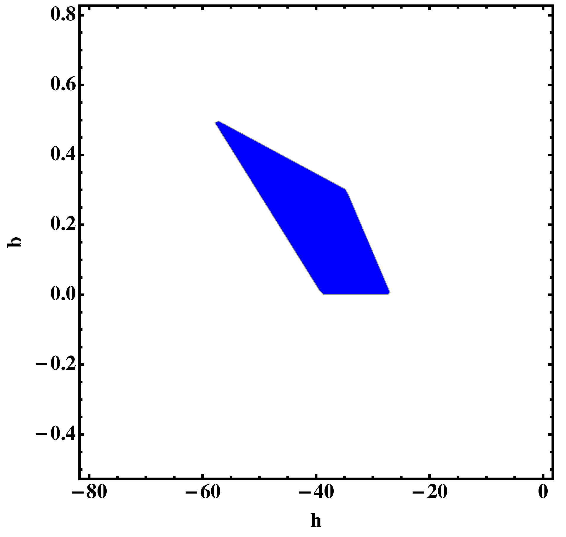
Here the inflationary parameters for the scalar and tensor fluctuations depend on the number of e-folds as well as on the value of the free parameters, particularly on b and on the combination $h=G_1/G_0+N$; thus in order to obtain some constrains for the values of b and h, we use the Planck and BICEP2/Keck Array data as above. The allowed region for the free parameters is shown in Figure 1, which shows the $1\sigma$ region for the spectral index, while the values for the tensor-to-scalar ratio satisfy the constraint given by Equation (23) within the blue region of Figure 1. In addition, the values for the free parameters within the $1\sigma$ region are able to have a tensor-to-scalar ratio as small as required; for instance, when considering $h=-40$ and $b=0.0001$, this leads to $r\sim {10}^{-5}$.

3.3. Example 3

Finally, we consider the case in which the Hubble rate is given by the following function of the number of e-folds:

$$\begin{array}{c}\hfill H^2\left(N\right)=G_2{\mathrm{e}}^{\beta N}+G_3,\end{array}$$

(44)

where the constants $G_2>0$ and $G_3>0$. Following the same procedure as in the previous cases, the equation for $g\left(N\right)$ is obtained by inserting Equation (44) into Equation (14), which results in

$$\begin{array}{c}\tilde{C}{\mathrm{e}}^{3-3N}+{\mathrm{e}}^{N\beta }{G}_2\beta ({\mathrm{e}}^{N\beta }{G}_2+G_3)\hfill \\ +4{({\mathrm{e}}^{N\beta }{G}_2+G_3)}^3(G_3+{\mathrm{e}}^{N\beta }{G}_2(-1+3\beta ))g\left(N\right)\hfill \\ +4{({\mathrm{e}}^{N\beta }{G}_2+G_3)}^4{g}^{\prime }\left(N\right)=0.\hfill \end{array}$$

(45)

Before solving this equation, we constrain the parameters $G_2$, $G_3$, and $\beta$. We note that the slow-roll parameters now read

$$\begin{array}{ccc}\hfill ϵ& =& -\frac{\beta G_2{\mathrm{e}}^{\beta N}(G_2{\mathrm{e}}^{\beta N}+G_3)}{2{(G_2{\mathrm{e}}^{\beta N}+\frac{6G_3}{6+\beta })}^2},\hfill \end{array}$$

(46)

$$\begin{array}{ccc}\hfill \eta & =& -\frac{\beta (2G_2{\mathrm{e}}^{\beta N}+G_3)}{2(G_2{\mathrm{e}}^{\beta N}+\frac{6G_3}{6+\beta })}.\hfill \end{array}$$

(47)

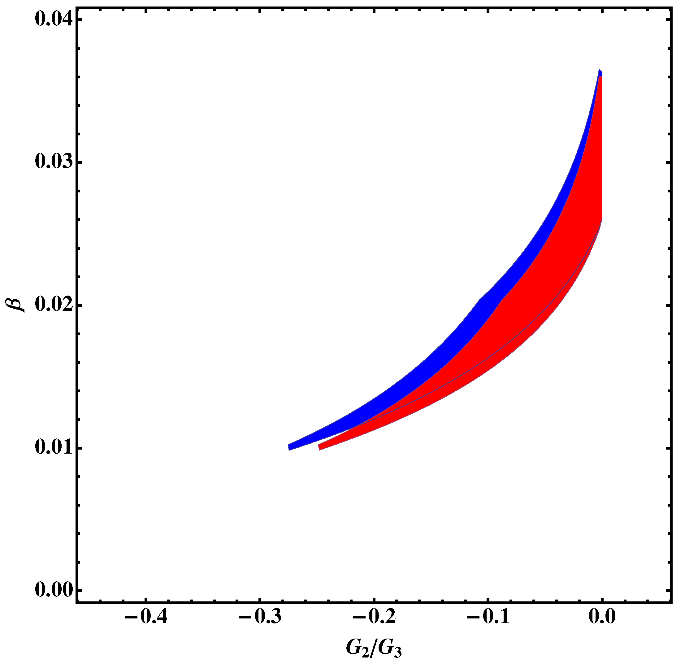
Here, the spectral index $n_s$ and the tensor-to-scalar ratio r (Equation (20)) depend on the number of e-folds, the parameter $\beta$, and the ratio $G_2/G_3$; thus in order to obtain some information about the value of the free parameters by using the Planck data and BICEP2/Keck Array data as before, we consider two samples, depending on the number of e-folds during inflation. In Figure 2, we consider the cases $N=50$ and $N=60$.

As shown in the figure, the parameters are well constrained, particularly the value of the exponent $\beta$.

In order to reconstruct the gravitational action analytically, we assume some approximations that can simplify the equations. Otherwise, it is not possible to obtain the mimetic Gauss–Bonnet Lagrangian exactly for this case as above. Thus, as $\beta \sim 0.03$ seems to be natural, and, combined with the slow-roll condition $|\dot{H}|\ll H^2$, we obtain $\frac{G_2{\mathrm{e}}^{\beta N}}{G_3}\gg 1$, such that the Hubble parameter (Equation (44)) can be approximated as follows:

$$\begin{array}{c}{H}^2\left(N\right)\simeq G_2{\mathrm{e}}^{\beta N}.\hfill \end{array}$$

(48)

The Gauss–Bonnet invariant is given by

$$\begin{array}{c}\hfill \mathcal{G}\left(N\right)\simeq -24(1+\beta )G_2^4{\mathrm{e}}^{4N\beta }.\end{array}$$

(49)

Then, Equation (45) takes the form

$$\begin{array}{c}\hfill \tilde{C}{\mathrm{e}}^{3-3N}+{\mathrm{e}}^{n\beta }{G}_2\beta {\mathrm{e}}^{N\beta }{G}_2+4{\mathrm{e}}^{4N\beta }{G}_2^4(-1+3\beta )g\left(N\right)+4{\mathrm{e}}^{N\beta }{G}_2^4{g}^{\prime }\left(N\right)\simeq 0.\end{array}$$

(50)

By following the same procedure as above, the approximate form for $f\left(\mathcal{G}\right)$ leads to

$$\begin{array}{c}\hfill f\left(\mathcal{G}\left(N\right)\right)\sim 24G_2^3\beta (1-\beta )\frac{{\mathrm{e}}^{N\beta }}{3G_2^2\beta (\beta -1)}+\frac{\tilde{C}{\mathrm{e}}^{3-3N-N\beta }}{G_2^4(3+\beta )(4+\beta )(3+5\beta )}+\frac{c_1{\mathrm{e}}^N}{1-4\beta },\end{array}$$

(51)

which in terms of the Gauss–Bonnet invariant leads to

$$\begin{array}{ccc}f\left(\mathcal{G}\right(N\left)\right)& =& 24G_2^3\beta (1-\beta )\left\{\frac{{\left[-\mathcal{G}/24(1+\beta )\right]}^{1/4}}{3G_2^3\beta (\beta -1)}+\tilde{C}{\mathrm{e}}^3\frac{{\left[-\mathcal{G}/24G_2^4(1+\beta )\right]}^{-(3+\beta )/4\beta }}{G_2^4(3+\beta )(4+\beta )(3+5\beta )}\right.\hfill \\ & & \left.+\frac{c_1{\left[-\mathcal{G}/24G_2^4(1+\beta )\right]}^{1/4\beta }}{1-4\beta }\right\}.\hfill \end{array}$$

(52)

The explicit form for the mimetic Gauss–Bonnet Lagrangian is thus obtained.

4. Extensions of Mimetic f(G) Gravity

We now consider some extensions of mimetic f(G) gravity and the reconstruction of inflationary models within such extensions. An alternative way of representing mimetic gravity relies on the use of a constraint equation that can be expressed through a Lagrange multiplier in the action [62,66]:

$$\begin{array}{c}\hfill S=\int d^{4}x\sqrt{-g}\left[\frac{R}{2{\kappa }^2}+f\left(\mathcal{G}\right)+\lambda (g^{\mu \nu }{\partial }_{\mu }\varphi {\partial }_{\nu }\varphi +1)\right].\end{array}$$

(53)

The variation with respect to the Lagrange multiplier $\lambda$ recovers Equation (2). Then, it is straightforward to show that the field equations for mimetic $f\left(\mathcal{G}\right)$ gravity (Equation (7)) are recovered. Nevertheless, here we are interested in analysing some extensions for the mimetic action (Equation (53)) by adding a kinetic term and a potential for the scalar field to make it dynamical:

$$\begin{array}{c}\hfill S=\int d^{4}x\sqrt{-g}\left[\frac{R}{2{\kappa }^2}+f\left(\mathcal{G}\right)-ϵg^{\mu \nu }{\partial }_{\mu }\varphi {\partial }_{\nu }\varphi -V\left(\varphi \right)+\lambda (g^{\mu \nu }{\partial }_{\mu }\varphi {\partial }_{\nu }\varphi +1)\right],\end{array}$$

(54)

By assuming again the spatially flat FLRW metric (Equation (9)), the variation of the action given by Equation (54) with respect to the metric $g_{\mu \nu }$ gives rise to the following equations of motion:

$$3H^2+24H^3\frac{d{f}_{\mathcal{G}}(\mathcal{G})}{dt}+f(\mathcal{G})-f_{\mathcal{G}}(\mathcal{G})\mathcal{G}=ϵ{\dot{\varphi }}^2+V(\varphi )-\lambda ({\dot{\varphi }}^2+1),$$

(55)

$$-2\dot{H}-3H^2-8H^2\frac{d^2{f}_{\mathcal{G}}(\mathcal{G})}{d{t}^2}-16H(\dot{H}+H^2)\frac{d{f}_{\mathcal{G}}(\mathcal{G})}{dt}+f_{\mathcal{G}}(\mathcal{G})\mathcal{G}-f(\mathcal{G})=ϵ{\dot{\varphi }}^2+-V(\varphi )-\lambda ({\dot{\varphi }}^2-1),$$

(56)

while the variation with respect to the Lagrange multiplier $\lambda$ yields the constraint for the scalar field $\varphi$:

$$\begin{array}{c}\hfill {\dot{\varphi }}^2-1=0.\end{array}$$

(57)

By redefining the mimetic scalar field as cosmic time $\varphi =t$, and by combining Equations (55) and (56), the scalar potential and the Lagrange multiplier can be expressed as functions of cosmological time t in terms of the Hubble parameter:

$$\begin{array}{ccc}\hfill V\left(t\right)& =& 2\dot{H}+3H^2+ϵ{\dot{\varphi }}^2+8H^2\frac{d^2{f}_{\mathcal{G}}\left(\mathcal{G}\right)}{d{t}^2}+16H(\dot{H}+H^2)\frac{d{f}_{\mathcal{G}}\left(\mathcal{G}\right)}{dt}-f_{\mathcal{G}}\left(\mathcal{G}\right)\mathcal{G}+f\left(\mathcal{G}\right),\hfill \end{array}$$

(58)

$$\begin{array}{ccc}\hfill \lambda \left(t\right)& =& {\dot{\varphi }}^{-2}\left(\frac{\rho }{2}+\dot{H}+4H(2\dot{H}-H^2)\frac{d{f}_{\mathcal{G}}\left(\mathcal{G}\right)}{dt}+4H^2\frac{d^2{f}_{\mathcal{G}}\left(\mathcal{G}\right)}{d{t}^2}\right)+ϵ.\hfill \end{array}$$

(59)

Hence, the particular action (Equation (54)) can be easily reconstructed for any cosmological model once the Hubble parameter is provided, as shown below for the examples studied in the previous section. Nevertheless, it is more convenient to express the potential V and the Lagrange multiplier $\lambda$ in terms of the e-folding number N instead of the cosmological time t, such that Equations (58) and (59) can be written as follows:

$$\begin{array}{ccc}V\left(N\right)& =& 2H\left(N\right)H^{\prime }\left(N\right)+3H{\left(N\right)}^2+ϵH{\left(N\right)}^2{\dot{\varphi }}^2+8H{\left(N\right)}^2\left[H{\left(N\right)}^2\frac{d^2}{d{N}^2}+H\left(N\right)H^{\prime }\left(N\right)\frac{d}{dN}\right]f_{\mathcal{G}}\left(\mathcal{G}\right)\hfill \\ & & +16H{\left(N\right)}^3\left[H^{\prime }\left(N\right)+H\left(N\right)\right]\frac{d{f}_{\mathcal{G}}\left(\mathcal{G}\right)}{dN}-f_{\mathcal{G}}\left(\mathcal{G}\right)\mathcal{G}+f\left(\mathcal{G}\right),\hfill \end{array}$$

(60)

$$\begin{array}{ccc}\lambda \left(N\right)& =& \frac{\rho }{2}+4H\left(N\right)H^{\prime }\left(N\right)+H{\left(N\right)}^3\left[2H^{\prime }\left(N\right)-H\left(N\right)\right]\frac{d{f}_{\mathcal{G}}\left(\mathcal{G}\right)}{dN}\hfill \\ & & +4H{\left(N\right)}^2\left[H{\left(N\right)}^2\frac{d^2}{d{N}^2}+H\left(N\right)H^{\prime }\left(N\right)\frac{d}{dN}\right]f_{\mathcal{G}}\left(\mathcal{G}\right)+ϵ.\hfill \end{array}$$

(61)

Alternatively, the function $f\left(\mathcal{G}\right)$ in the action given by Equation (54) can be expressed in terms of an extra auxiliary field by rewriting the action as follows:

$$\begin{array}{c}\hfill S=\int d^{4}x\sqrt{-g}\left[\frac{R}{2{\kappa }^2}+\phi \mathcal{G}-U\left(\phi \right)-V\left(\varphi \right)+\lambda (g^{\mu \nu }{\partial }_{\mu }\varphi {\partial }_{\nu }\varphi +1)\right],\end{array}$$

(62)

where $\phi =f^{\prime }\left(\mathcal{G}\right)$ and we have omitted the kinetic term for $\varphi$ for simplicity. The variation of the action with respect to $g_{\mu \nu }$ gives the following field equations:

$$\begin{array}{c}\hfill R_{\mu \nu }-\frac{1}{2}R{g}_{\mu \nu }+U\left(\phi \right)g_{\mu \nu }+2H_{\mu \nu }-\left[\lambda (g^{\mu \nu }{\partial }_{\mu }\varphi {\partial }_{\nu }\varphi +1)-V\left(\varphi \right)\right]g_{\mu \nu }+2\lambda {\partial }_{\mu }\varphi {\partial }_{\nu }\varphi =0.\end{array}$$

(63)

Here the term $H_{\mu \nu }$ is the variation of $\phi \mathcal{G}$:

$$\begin{array}{ccc}\hfill H_{\mu \nu }& \equiv & \frac{1}{\sqrt{-g}}\frac{\delta \left(\sqrt{-g}\phi \mathcal{G}\right)}{\delta g^{\mu \nu }}\hfill \\ & =& 2R(g_{\mu \nu }\square -{\nabla }_{\mu }{\nabla }_{\nu })\phi +4R_{\mu }^{\alpha }{\nabla }_{\alpha }{\nabla }_{\nu }\phi +4R_{\nu }^{\alpha }{\nabla }_{\alpha }{\nabla }_{\mu }\phi \hfill \\ & & -4R_{\mu \nu }\square \phi -4g_{\mu \nu }{R}^{\alpha \beta }{\nabla }_{\alpha }{\nabla }_{\beta }\phi +4R_{\alpha \mu \beta \nu }{\nabla }^{\alpha }{\nabla }^{\beta }\phi ,\hfill \end{array}$$

(64)

whereas the constraint of the mimetic scalar is given by Equation (57). The FLRW equations for the action given by Equation (63) turn out to be

$$\begin{array}{c}3H{\left(t\right)}^2(1+8H\left(t\right){\phi }^{\prime }\left(t\right))+\lambda \left(t\right)(1+{\varphi }^{\prime }{\left(t\right)}^2)-V\left(\varphi \left(t\right)\right)-U\left(\phi \left(t\right)\right)=0\hfill \\ H\left(t\right)\left[16H{\left(t\right)}^2{\phi }^{\prime }\left(t\right)+16\dot{H}\left(t\right){\phi }^{\prime }\left(t\right)+H\left(t\right)(3+8{\phi }^{\prime \prime }\left(t\right))\right]\hfill \end{array}$$

(65)

$$\begin{array}{c}+\lambda \left(t\right)\left[1-{\varphi }^{\prime }{\left(t\right)}^2\right]+2\dot{H}\left(t\right)-V\left(\varphi \left(t\right)\right)-U\left(\phi \left(t\right)\right)=0.\hfill \end{array}$$

(66)

It is straightforward to obtain the Hubble parameter from Equation (65), leading to the following solution:

$$\begin{array}{c}\hfill H\left(N\right)=\sqrt{\pm \frac{\sqrt{9-96{\phi }^{\prime }\left(N\right)(2\lambda \left(N\right)-U\left(\phi \left(N\right)\right)-V\left(\varphi \left(N\right)\right))}}{48{\phi }^{\prime }\left(N\right)}-\frac{1}{16{\phi }^{\prime }\left(N\right)}}.\end{array}$$

(67)

In the following, the full action (Equation (54)) is reconstructed for some inflationary models. Because the action (Equation (54)) retains more degrees of freedom, we assume a particular ansazt for the function $f\left(\mathcal{G}\right)$, the simplest possible choice, which is given by

$$\begin{array}{c}\hfill f\left(\mathcal{G}\right)=A{\mathcal{G}}^2.\end{array}$$

(68)

Then, by Equations (60) and (61), the corresponding action is recovered.

We first consider a simple example, a subclass of the first case studied above, for which the cosmological evolution is described by the following Hubble parameter:

$$\begin{array}{c}\hfill H^2\left(N\right)=G_{0}N+G_1.\end{array}$$

(69)

Substituting Equation (69) into Equations (60) and (61) and recalling that $\varphi =t$, we obtain the potential for the scalar field in terms of the number of e-folds:

$$\begin{array}{ccc}V\left(N\right)& =& -768A{G}_0^2{(G_{0}N+G_1)}^2-12A{G}_0^2(4G_{0}N+G_0+4G_1)\hfill \\ & & -192A{G}_0(G_{0}N+G_1)(2G_{0}N+G_0+2G_1)(4G_{0}N+G_0+4G_1)\hfill \\ & & -288A{(G_{0}N+G_1)}^2{(2G_{0}N+G_0+2G_1)}^2-24A(G_{0}N+G_1)(2G_{0}N+G_0+2G_1)r\hfill \\ & & +3(G_{0}N+G_1)+G_0+ϵ,\hfill \end{array}$$

(70)

while the configuration of the Lagrange multiplier yields

$$\begin{array}{ccc}\lambda \left(N\right)& =& \frac{1}{2}{G}_0(1+96A(G_1+G_{0}N)(8G_1^2+2G_0{G}_1(-9+8N)\hfill \\ & & +G_0^2(-3+2N(-9+4N))\left)\right)+ϵ.\hfill \end{array}$$

(71)

The scalar field as a function of N is obtained by using $\frac{dN}{dt}=H\left(N\right)$ and $\varphi =t$, leading to

$$\begin{array}{c}\hfill \varphi \left(N\right)=-\frac{2(\sqrt{G_0+G_1}-\sqrt{G_1+G_{0}N})}{G_0}.\end{array}$$

(72)

Hence, by combining Equations (70) and (72), we obtain the potential $V\left(\varphi \right)$:

$$\begin{array}{ccc}V\left(\varphi \right)& =& -768A{G}_0^2{\left(\frac{G_0^2{\varphi }^2}{4}+G_0\varphi \sqrt{G_0+G_1}+G_0+G_1\right)}^2\hfill \\ & & -12A{G}_0^2\left(G_0\left(4\varphi \sqrt{G_0+G_1}+G_0{\varphi }^2+5\right)+4G_1\right)\hfill \\ & & -24A{G}_0\left(G_0\left(4\varphi \sqrt{G_0+G_1}+G_0{\varphi }^2+4\right)+4G_1\right)\left(G_0\left(4\varphi \sqrt{G_0+G_1}+G_0{\varphi }^2+5\right)+4G_1\right)\hfill \\ & & \times \left(G_0\left(4\varphi \sqrt{G_0+G_1}+G_0{\varphi }^2+6\right)+4G_1\right)\hfill \\ & & -\frac{9}{2}A{\left(G_0\left(4\varphi \sqrt{G_0+G_1}+G_0{\varphi }^2+4\right)+4G_1\right)}^2{\left(G_0\left(4\varphi \sqrt{G_0+G_1}+G_0{\varphi }^2+6\right)+4G_1\right)}^2\hfill \\ & & -3A\left(G_0\left(4\varphi \sqrt{G_0+G_1}+G_0{\varphi }^2+4\right)+4G_1\right)\left(G_0\left(4\varphi \sqrt{G_0+G_1}+G_0{\varphi }^2+6\right)+4G_1\right)\hfill \\ & & +3\left(\frac{G_0^2{\varphi }^2}{4}+G_0\varphi \sqrt{G_0+G_1}+G_0+G_1\right)+G_0+ϵ.\hfill \end{array}$$

(73)

Finally, we consider the third example studied above, where we recall that the cosmological evolution is given by $H^2\left(N\right)=-G_2{\mathrm{e}}^{\beta N}+G_3$. Similarly to the previous case, the scalar potential and the Lagrange multiplier in terms of the number of e-folds N are obtained:

$$\begin{array}{ccc}\hfill V\left(N\right)& =& -96A(\beta +2)\left(\beta (12\beta +11)+6\right)G_2^4{e}^{4\beta N})\hfill \\ & & -24A{G}_2^3\left((\beta +2){\beta }^2+8(\beta (\beta (12\beta +41)+42)+24)G_3\right)e^{3\beta N})\hfill \\ & & -12A{G}_2^2\left(2(\beta +2)+8(\beta (\beta (14\beta +59)+84)+72)G_3^2+{\beta }^2(\beta +4)G_3\right)e^{2\beta N})\hfill \\ & & -G_2{e}^{\beta N}\left(24A(\beta +4)G_3\left(8(\beta (\beta +2)+6)G_3^2+1\right)-\beta -3\right))\hfill \\ & & -3G_3\left(16A\left(24G_3^3+G_3\right)-1\right)+ϵ,\hfill \end{array}$$

(74)

$$\begin{array}{ccc}\hfill \lambda \left(N\right)& =& -96A(\beta +2)(\beta (12\beta +11)+6)G_2^4{e}^{4\beta N})\hfill \\ & & -24A{G}_2^3\left((\beta +2){\beta }^2+8(\beta (\beta (12\beta +41)+42)+24)G_3\right)e^{3\beta N})\hfill \\ & & -12A{G}_2^2\left(2(\beta +2)+8(\beta (\beta (14\beta +59)+84)+72)G_3^2+{\beta }^2(\beta +4)G_3\right)e^{2\beta N})\hfill \\ & & -G_2{e}^{\beta N}\left(24A(\beta +4)G_3\left(8(\beta (\beta +2)+6)G_3^2+1\right)-\beta -3\right))\hfill \\ & & -3G_3\left(16A\left(24G_3^3+G_3\right)-1\right)+ϵ,\hfill \end{array}$$

(75)

whereas the scalar field yields

$$\begin{array}{ccc}\hfill \varphi \left(N\right)& =& \frac{2\mathrm{arctanh}\left(\frac{\sqrt{{\mathrm{e}}^{\beta }{G}_2+G_3}}{\sqrt{G_3}}\right)-2\mathrm{arctanh}\left(\frac{\sqrt{{\mathrm{e}}^{\beta N}{G}_2+G_3}}{\sqrt{G_3}}\right)}{\beta \sqrt{G_3}}.\hfill \end{array}$$

(76)

Finally, the potential $V\left(\varphi \right)$ can be expressed as a function of $\varphi$, as follows:

$$\begin{array}{ccc}V\left(\varphi \right)& =& -96A{G}_3^4(W\left(\varphi \right)-1)\left(\left(12{\beta }^3+35{\beta }^2+28\beta +12\right)W{\left(\varphi \right)}^3\right.\hfill \\ & & \left.-\left(12{\beta }^3+47{\beta }^2+56\beta +36\right)W{\left(\varphi \right)}^2+2\left({\beta }^3+6{\beta }^2+14\beta +18\right)W\left(\varphi \right)-12\right)\hfill \\ & & +12A{\beta }^2{G}_3^{3}W{\left(\varphi \right)}^2(-\beta +2(\beta +2)W\left(\varphi \right)-4)\hfill \\ & & -24A{G}_3^2(W\left(\varphi \right)-1)((\beta +2)W-2)-G_3((\beta +3)W\left(\varphi \right)-3)+ϵ,\hfill \end{array}$$

(77)

where $W\left(\varphi \right)=\sec \mathrm{h}{\left(\frac{1}{2}\sqrt{G_3}\beta \varphi -\mathrm{arctanh}\left(\frac{\sqrt{{\mathrm{e}}^{\beta }{G}_2+G_3}}{\sqrt{G_3}}\right)\right)}^2$. Hence, we have shown that any inflationary model can be easily obtained from the mimetic action (Equation (54)).

5. Conclusions

As shown previously in the literature, Gauss–Bonnet gravity can easily reproduce any model of inflation by assuming the appropriate gravitational action. Here we have extended such an analysis by assuming the mimetic condition, which isolates the conformal degree of freedom through an auxiliary scalar field that behaves as a pressureless fluid in homogeneous and isotropic cosmologies. Then, we have assumed the Hilbert–Einstein action with a correction in the form of a function of the Gauss–Bonnet invariant. By some analytical techniques, we have reconstructed the appropriate $f\left(\mathcal{G}\right)$ actions for some inflationary models, which reproduce slow-roll inflation. The predictions of such models have also been analysed by obtaining the values for the spectral index and the tensor-to-scalar ratio. As shown by the results, model 1 provides a spectral index slightly higher than that provided by Planck, while models 2 and 3 correctly fit the observational constraints, despite that it is not possible for the analytical form of the gravitational action to be obtained for the former, although it is for the latter. In comparison to standard Gauss–Bonnet gravities, mimetic gravity introduces an additional degree of freedom that behaves as a pressureless fluid, leading to greater complexity of the equations, which allows us to avoid reconstructing the exact gravitational action for some cases. Nevertheless, we have shown that even with the presence of such a fluid, inflation can be realised in mimetic Gauss–Bonnet gravity.

We have also explored some analytical extensions of mimetic Gauss–Bonnet gravity by adding a kinetic term and a potential to the auxiliary scalar field. For this aim, we have used the approach of the Lagrange multiplier, equivalent to the mimetic condition. We note that as the auxiliary field becomes dynamical and the $f\left(\mathcal{G}\right)$ action can be expressed in terms of another scalar field, inflation becomes equivalent to a multifield model, for which isocurvature (non-adiabatic) perturbations may not be null [86,87,88]; this is an aspect that requires a further and exclusive analysis in a future work. Nevertheless, by analysing the same inflationary models, the corresponding scalar potential has been reconstructed, whereby we have assumed $f\left(\mathcal{G}\right)\propto {\mathcal{G}}^2$ for simplicity.

Finally, an interesting point to be considered would be the analysis of loop quantum cosmology corrections within mimetic modified gravities. As shown in [89,90] for classical extensions of GR, such corrections may discard some inflationary/bouncing models, providing some more accurate gravitational actions for the corresponding cosmological solutions.

Hence, we have shown that inflation can be realised in Gauss–Bonnet gravity when incorporating the mimetic condition, and viable inflationary models that satisfy the latest observational constraints can be reconstructed, which opens up new means to explore the early universe in the framework of this type of theory.

References

- Liddle, A.R.; Lyth, D.H. Cosmological Inflation and Large-Scale Structure; Cambridge University Press: Cambridge, UK, 2000. [Google Scholar]
- Dodelson, S. Modern Cosmology; Academic Press: Cambridge, MA, USA, 1999. [Google Scholar]
- Mukhanov, V.F.; Feldman, H.A.; Brandenberger, R.H. Theory of cosmological perturbations. Part 1. Classical perturbations. Part 2. Quantum theory of perturbations. Part 3. Extensions. Phys. Rept. 1992, 215, 203. [Google Scholar] [CrossRef]
- Liddle, A.R. An Introduction to cosmological inflation. arXiv, 1998; arXiv:astro-ph/9901124. [Google Scholar]
- Langlois, D. Lectures on inflation and cosmological perturbations. Lect. Notes Phys. 2010, 800, 1. [Google Scholar] [CrossRef]
- Khoury, J.; Ovrut, B.A.; Steinhardt, P.J.; Turok, N. The Ekpyrotic universe: Colliding branes and the origin of the hot big bang. Phys. Rev. D 2001, 64, 123522. [Google Scholar] [CrossRef]
- Khoury, J.; Ovrut, B.A.; Steinhardt, P.J.; Turok, N. Density perturbations in the ekpyrotic scenario. Phys. Rev. D 2002, 66, 046005. [Google Scholar] [CrossRef]
- Peiris, H.V.; Komatsu, E.; Verde, L.; Spergel, D.N.; Bennett, C.L.; Halpern, M.; Hinshaw, G.; Jarosik, N.; Kogut, A.; Limon, M.; et al. First year Wilkinson Microwave Anisotropy Probe (WMAP) observations: Implications for inflation. Astrophys. J. Suppl. 2003, 148, 213. [Google Scholar] [CrossRef]
- Hinshaw, G.; Larson, D.; Komatsu, E.; Spergel, D.N.; Bennett, C.L.; Dunkley, J.; Nolta, M.R.; Halpern, M.; Hill, R.S.; Odegard, N.; et al. Nine-Year Wilkinson Microwave Anisotropy Probe (WMAP) Observations: Cosmological Parameter Results. Astrophys. J. Suppl. 2013, 208, 19. [Google Scholar] [CrossRef]
- Ade, P.A.R.; Aghanim, N.; Arnaud, M.; Arroja, F.; Ashdown, M.; Aumont, J.; Baccigalupi, C.; Ballardini, M.; Banday, A.J.; Barreiro, R.B.; et al. Planck 2015 results. XX. Constraints on inflation.’ Astron. Astrophys. 2016, 594, A20. [Google Scholar] [CrossRef]
- Ade, P.A.R.; Ahmed, Z.; Aikin, R.W.; Alexander, K.D.; Barkats, D.; Benton, S.J.; Bischoff, C.A.; Bock, J.J.; Bowens-Rubin, R.; Brevik, J.A.; Buder, I.; et al. Improved Constraints on Cosmology and Foregrounds from BICEP2 and Keck Array Cosmic Microwave Background Data with Inclusion of 95 GHz Band. Phys. Rev. Lett. 2016, 116. [Google Scholar] [CrossRef] [PubMed]
- Lidsey, J.E.; Liddle, A.R.; Kolb, E.W.; Copeland, E.J.; Barreiro, T.; Abney, M. Reconstructing the inflation potential: An overview. Rev. Mod. Phys. 1997, 69, 373. [Google Scholar] [CrossRef]
- Elizalde, E.; Nojiri, S.; Odintsov, S.D.; Saez-Gomez, D.; Faraoni, V. Reconstructing the universe history, from inflation to acceleration, with phantom and canonical scalar fields. Phys. Rev. D 2008, 77, 106005. [Google Scholar] [CrossRef]
- Nojiri, S.; Odintsov, S.D. Unified cosmic history in modified gravity: From F(R) theory to Lorentz non-invariant models. Phys. Rept. 2011, 505, 59–144. [Google Scholar] [CrossRef]
- Nojiri, S.; Odintsov, S.D. Introduction to modified gravity and gravitational alternative for dark energy. Int. J. Geom. Meth. Mod. Phys. 2007, 4, 115–145. [Google Scholar] [CrossRef]
- Capozziello, S.; De Laurentis, M. Extended Theories of Gravity. Phys. Rept. 2011, 509, 167–321. [Google Scholar] [CrossRef]
- Capozziello, S.; Faraoni, V. Beyond Einstein Gravity; Springer: Dordrecht, The Netherlands, 2010. [Google Scholar]
- De la Cruz-Dombriz, A.; Sáez-Gómez, D. Black holes, cosmological solutions, future singularities, and their thermodynamical properties in modified gravity theories. Entropy 2012, 14, 1717–1770. [Google Scholar] [CrossRef] [Green Version]
- Clifton, T.; Ferreira, P.G.; Padilla, A.; Skordis, C. Modified gravity and cosmology. Phys. Rept. 2012, 513, 1–189. [Google Scholar] [CrossRef]
- Capozziello, S.; De Laurentis, M.; Faraoni, V. ‘A bird’s eye view of f(R)-gravity. arXiv, 2009; arXiv:0909.4672v2. [Google Scholar]
- Nojiri, S.; Odintsov, S.D.; Oikonomou, V.K. Modified Gravity Theories on a Nutshell: Inflation, Bounce and Late-time Evolution. Phys. Rept. 2017, 692, 1–104. [Google Scholar] [CrossRef]
- Olmo, G.J. Palatini Approach to Modified Gravity: F(R) Theories and Beyond. Int. J. Mod. Phys. D 2011, 20, 413–462. [Google Scholar] [CrossRef]
- Beltran Jimenez, J.; Heisenberg, L.; Olmo, G.J.; Rubiera-Garcia, D. Born-Infeld inspired modifications of gravity. Phys. Rept. 2018, 727, 1. [Google Scholar] [CrossRef]
- Bamba, K.; Nojiri, S.; Odintsov, S.D.; Sáez-Gómez, D. Inflationary universe from perfect fluid and F(R) gravity and its comparison with observational data. Phys. Rev. D 2014, 90, 124061. [Google Scholar] [CrossRef]
- Starobinsky, A.A. A New Type of Isotropic Cosmological Models Without Singularity. Phys. Lett. B 1980, 91, 99. [Google Scholar] [CrossRef]
- De la Cruz-Dombriz, A.; Elizalde, E.; Odintsov, S.D.; Sáez-Gómez, D. Spotting deviations from R2 inflation. J. Cosmol. Astropart. Phys. 2016, 1605, 060. [Google Scholar] [CrossRef]
- Cognola, G.; Elizalde, E.; Nojiri, S.; Odintsov, S.D.; Sebastiani, L.; Zerbini, S. A Class of viable modified f(R) gravities describing inflation and the onset of accelerated expansion. Phys. Rev. D 2008, 77, 046009. [Google Scholar] [CrossRef]
- Nojiri, S.; Odintsov, S.D. Modified f(R) gravity unifying R**m inflation with Lambda CDM epoch. Phys. Rev. D 2008, 77, 026007. [Google Scholar] [CrossRef]
- Cognola, G.; Elizalde, E.; Odintsov, S.D.; Tretyakov, P.; Zerbini, S. Initial and final de Sitter universes from modified f(R) gravity. Phys. Rev. D 2009, 79, 044001. [Google Scholar] [CrossRef]
- Odintsov, S.D.; Sáez-Chillón Gómez, D.; Sharov, G.S. Is exponential gravity a viable description for the whole cosmological history? Eur. Phys. J. C 2017, 77, 862. [Google Scholar] [CrossRef] [PubMed]
- Harko, T.; Lobo, F.S.N.; Nojiri, S.; Odintsov, S.D. f(R,T) gravity. Phys. Rev. D 2011, 84, 024020. [Google Scholar] [CrossRef]
- Odintsov, S.D.; Sáez-Gómez, D. f(R,T,RμνTμν) gravity phenomenology and ΛCDM universe. Phys. Lett. B 2013, 725, 437–444. [Google Scholar] [CrossRef]
- Haghani, Z.; Harko, T.; Lobo, F.S.N.; Sepangi, H.R.; Shahidi, S. Further matters in space-time geometry: F(R,T,RμνTμν) gravity. Phys. Rev. D 2013, 88, 044023. [Google Scholar] [CrossRef]
- Tamanini, N.; Koivisto, T.S. Consistency of nonminimally coupled f(R) gravity. Phys. Rev. D 2013, 88, 064052. [Google Scholar] [CrossRef]
- Alvarenga, F.G.; de la Cruz-Dombriz, A.; Houndjo, M.J.S.; Rodrigues, M.E.; Sáez-Gómez, D. Dynamics of scalar perturbations in f(R,T) gravity. Phys. Rev. D 2013, 87, 103526. [Google Scholar] [CrossRef] [Green Version]
- Nojiri, S.; Odintsov, S.D.; Sasaki, M. Gauss-Bonnet dark energy. Phys. Rev. D 2005, 71, 123509. [Google Scholar] [CrossRef]
- Nojiri, S.; Odintsov, S.D. Modified Gauss-Bonnet theory as gravitational alternative for dark energy. Phys. Lett. B 2005, 631, 1–6. [Google Scholar] [CrossRef]
- Cognola, G.; Elizalde, E.; Nojiri, S.; Odintsov, S.D.; Zerbini, S. Dark energy in modified Gauss-Bonnet gravity: Late-time acceleration and the hierarchy problem. Phys. Rev. D 2006, 73, 084007. [Google Scholar] [CrossRef]
- Calcagni, G.; De Carlos, B.; De Felice, A. Ghost conditions for Gauss-Bonnet cosmologies. Nucl. Phys. B 2006, 752, 404–438. [Google Scholar] [CrossRef]
- Koivisto, T.; Mota, D.F. Gauss-Bonnet Quintessence: Background Evolution, Large Scale Structure and Cosmological Constraints. Phys. Rev. D 2007, 75, 023518. [Google Scholar] [CrossRef]
- Leith, B.M.; Neupane, I.P. Gauss-Bonnet cosmologies: Crossing the phantom divide and the transition from matter dominance to dark energy. J. Cosmol. Astropart. Phys. 2007, 2007. [Google Scholar] [CrossRef]
- De la Cruz-Dombriz, A.; Saez-Gomez, D. On the stability of the cosmological solutions in f(R,G) gravity. Class. Quant. Grav. 2012, 29, 245014. [Google Scholar] [CrossRef]
- Elizalde, E.; Myrzakulov, R.; Obukhov, V.V.; Saez-Gomez, D. LambdaCDM epoch reconstruction from F(R,G) and modified Gauss-Bonnet gravities. Class. Quant. Grav. 2010, 27, 095007. [Google Scholar] [CrossRef]
- Myrzakulov, R.; Saez-Gomez, D.; Tureanu, A. On the ΛCDM Universe in f(G) gravity. Gen. Rel. Grav. 2011, 43, 1671. [Google Scholar] [CrossRef]
- Kanti, P.; Gannouji, R.; Dadhich, N. Gauss-Bonnet Inflation. Phys. Rev. D 2015, 92, 041302. [Google Scholar] [CrossRef]
- Kanti, P.; Gannouji, R.; Dadhich, N. Early-time cosmological solutions in Einstein-scalar-Gauss-Bonnet theory. Phys. Rev. D 2015, 92, 083524. [Google Scholar] [CrossRef]
- Lahiri, S. Anisotropic inflation in Gauss-Bonnet gravity. J. Cosmol. Astropart. Phys. 2016, 1609, 025. [Google Scholar] [CrossRef]
- Hikmawan, G.; Soda, J.; Suroso, A.; Zen, F.P. Comment on ?Gauss-Bonnet inflation? Phys. Rev. D 2016, 93, 068301. [Google Scholar] [CrossRef]
- Satoh, M. Slow-roll Inflation with the Gauss-Bonnet and Chern-Simons Corrections. J. Cosmol. Astropart. Phys. 2010, 1011. [Google Scholar] [CrossRef]
- Guo, Z.K.; Schwarz, D.J. Power spectra from an inflaton coupled to the Gauss-Bonnet term. Phys. Rev. D 2009, 80, 063523. [Google Scholar] [CrossRef]
- Koh, S.; Lee, B.H.; Lee, W.; Tumurtushaa, G. Observational constraints on slow-roll inflation coupled to a Gauss-Bonnet term. Phys. Rev. D 2014, 90, 063527. [Google Scholar] [CrossRef]
- Oikonomou, V.K. Singular Bouncing Cosmology from Gauss-Bonnet Modified Gravity. Phys. Rev. D 2015, 92, 124027. [Google Scholar] [CrossRef]
- De Felice, A.; Tanaka, T. Inevitable Ghost and the Degrees of Freedom in f(R, G) Gravity. Prog. Theor. Phys. 2010, 124, 503–515. [Google Scholar] [CrossRef]
- Feng, J.L. Dark Matter Candidates from Particle Physics and Methods of Detection. Ann. Rev. Astron. Astrophys. 2010, 48, 495–545. [Google Scholar] [CrossRef]
- Sanders, R.H.; McGaugh, S.S. Modified Newtonian dynamics as an alternative to dark matter. Ann. Rev. Astron. Astrophys. 2002, 40, 263–317. [Google Scholar] [CrossRef]
- Bekenstein, J.D. Modified gravity vs dark matter: Relativistic theory for MOND. PoS JHW 2005, 2004, 012. [Google Scholar]
- Nojiri, S.; Odintsov, S.D. Dark energy, inflation and dark matter from modified F(R) gravity. arXiv, 2011; arXiv:0807.0685. [Google Scholar]
- Capozziello, S.; Cardone, V.F.; Troisi, A. Dark energy and dark matter as curvature effects. J. Cosmol. Astropart. Phys. 2006, 8. [Google Scholar] [CrossRef]
- Capozziello, S.; De Laurentis, M. The dark matter problem from f(R) gravity viewpoint. Ann. Phys. 2012, 524, 545–578. [Google Scholar] [CrossRef]
- Chamseddine, A.H.; Mukhanov, V. Mimetic Dark Matter. JHEP 2013, 1311, 135. [Google Scholar] [CrossRef]
- Chamseddine, A.H.; Mukhanov, V.; Vikman, A. Cosmology with Mimetic Matter. J. Cosmol. Astropart. Phys. 2014, 1406. [Google Scholar] [CrossRef]
- Golovnev, A. On the recently proposed Mimetic Dark Matter. Phys. Lett. B 2014, 728, 39–40. [Google Scholar] [CrossRef] [Green Version]
- Deruelle, N.; Rua, J. Disformal Transformations, Veiled General Relativity and Mimetic Gravity. J. Cosmol. Astropart. Phys. 2014, 1409. [Google Scholar] [CrossRef]
- Nojiri, S.; Odintsov, S.D. Mimetic F(R) gravity: Inflation, dark energy and bounce. Mod. Phys. Lett. A 2014, 29, 1450211. [Google Scholar] [CrossRef]
- Momeni, D.; Altaibayeva, A.; Myrzakulov, R. New Modified Mimetic Gravity. Int. J. Geom. Meth. Mod. Phys. 2014, 11, 1450091. [Google Scholar] [CrossRef]
- Astashenok, A.V.; Odintsov, S.D.; Oikonomou, V.K. Modified Gauss?Bonnet gravity with the Lagrange multiplier constraint as mimetic theory. Class. Quant. Grav. 2015, 32, 185007. [Google Scholar] [CrossRef]
- Nojiri, S.; Odintsov, S.D.; Oikonomou, V.K. Viable Mimetic Completion of Unified Inflation-Dark Energy Evolution in Modified Gravity. Phys. Rev. D 2016, 94, 104050. [Google Scholar] [CrossRef]
- Leon, G.; Saridakis, E.N. Dynamical behavior in mimetic F(R) gravity. J. Cosmol. Astropart. Phys. 2015, 1504. [Google Scholar] [CrossRef]
- Odintsov, S.D.; Oikonomou, V.K. Accelerating cosmologies and the phase structure of F(R) gravity with Lagrange multiplier constraints: A mimetic approach. Phys. Rev. D 2016, 93, 023517. [Google Scholar] [CrossRef]
- Sebastiani, L.; Vagnozzi, S.; Myrzakulov, R. Mimetic gravity: A review of recent developments and applications to cosmology and astrophysics. Adv. High Energy Phys. 2017, 2017, 3156915. [Google Scholar] [CrossRef]
- Myrzakulov, R.; Sebastiani, L.; Vagnozzi, S. Inflation in f(R,ϕ)-theories and mimetic gravity scenario. Eur. Phys. J. C 2015, 75, 444. [Google Scholar] [CrossRef]
- Bouhmadi-López, M.; Chen, C.Y.; Chen, P. Primordial Cosmology in Mimetic Born-Infeld Gravity. J. Cosmol. Astropart. Phys. 2017, 1711, 053. [Google Scholar] [CrossRef]
- Matsumoto, J.; Odintsov, S.D.; Sushkov, S.V. Cosmological perturbations in a mimetic matter model. Phys. Rev. D 2015, 91, 064062. [Google Scholar] [CrossRef]
- Chen, C.Y.; Bouhmadi-López, M.; Chen, P. Black hole solutions in mimetic Born-Infeld gravity. Eur. Phys. J. C 2018, 78, 59. [Google Scholar] [CrossRef] [PubMed]
- Capozziello, S. Curvature quintessence. Int. J. Mod. Phys. D 2002, 11, 483–491. [Google Scholar] [CrossRef]
- Capozziello, S.; Carloni, S.; Troisi, A. Quintessence without scalar fields, Recent Res. Dev. Astron. Astrophys. 2003, 1, 625. [Google Scholar]
- Carroll, S.M.; Duvvuri, V.; Trodden, M.; Turner, M.S. Is cosmic speed-up due to new gravitational physics? Phys. Rev. D 2004, 70, 043528. [Google Scholar] [CrossRef]
- Carloni, S.; Goswami, R.; Dunsby, P.K.S. A new approach to reconstruction methods in f(R) gravity. Class. Quant. Grav. 2012, 29, 135012. [Google Scholar] [CrossRef]
- Elizalde, E.; Saez-Gomez, D. F(R) cosmology in presence of a phantom fluid and its scalar-tensor counterpart: Towards a unified precision model of the universe evolution. Phys. Rev. D 2009, 80, 044030. [Google Scholar] [CrossRef]
- Goheer, N.; Larena, J.; Dunsby, P.K.S. Power-law cosmic expansion in f(R) gravity models. Phys. Rev. D 2009, 80, 061301. [Google Scholar] [CrossRef]
- Bamba, K.; Capozziello, S.; Nojiri, S.; Odintsov, S.D. Dark energy cosmology: The equivalent description via different theoretical models and cosmography tests. Astrophys. Space Sci. 2012, 342, 155. [Google Scholar] [CrossRef]
- Das, S.; Banerjee, N.; Dadhich, N. Curvature driven acceleration: A utopia or a reality? Class. Quant. Grav. 2006, 23, 4159. [Google Scholar] [CrossRef]
- Saez-Gomez, D. Modified f(R) gravity from scalar-tensor theory and inhomogeneous EoS dark energy. Gen. Rel. Grav. 2009, 41, 1527–1538. [Google Scholar] [CrossRef]
- Nojiri, S.; Odintsov, S.D.; Saez-Gomez, D. Cosmological reconstruction of realistic modified F(R) gravities. Phys. Lett. B 2009, 681, 74–80. [Google Scholar] [CrossRef]
- De la Cruz-Dombriz, A.; Dobado, A. A f(R) gravity without cosmological constant. Phys. Rev. D 2006, 74, 087501. [Google Scholar] [CrossRef]
- Sasaki, M.; Stewart, E.D. A General analytic formula for the spectral index of the density perturbations produced during inflation. Prog. Theor. Phys. 1996, 95, 71–78. [Google Scholar] [CrossRef]
- Garcia-Bellido, J.; Wands, D. Metric perturbations in two field inflation. Phys. Rev. D 1996, 53, 5437. [Google Scholar] [CrossRef]
- Garcia-Bellido, J.; Wands, D. Constraints from inflation on scalar—Tensor gravity theories. Phys. Rev. D 1995, 52, 6739. [Google Scholar] [CrossRef]
- Kleidis, K.; Oikonomou, V.K. Loop quantum cosmology-corrected Gauss? Bonnet singular cosmology. Int. J. Geom. Meth. Mod. Phys. 2017, 15, 1850064. [Google Scholar] [CrossRef]
- Odintsov, S.D.; Oikonomou, V.K.; Saridakis, E.N. Superbounce and Loop Quantum Ekpyrotic Cosmologies from Modified Gravity: F(R), F(G) and F(T) Theories. Ann. Phys. 2015, 363, 141–163. [Google Scholar] [CrossRef]
Figure 1.
Confidence region for the parameter values of and b to be consistent with the Planck data and Background Imaging of Cosmic Extragalactic Polarisation (BICEP2)/Keck Array; h and b are constrained inside the blue region.
Figure 2.
Constraints for the parameters and . We have assumed (blue) and (red). To be consistent with the Planck data and Background Imaging of Cosmic Extragalactic Polarisation (BICEP2)/Keck Array, and are constrained inside the coloured areas.
© 2018 by the authors. Licensee MDPI, Basel, Switzerland. This article is an open access article distributed under the terms and conditions of the Creative Commons Attribution (CC BY) license (http://creativecommons.org/licenses/by/4.0/).
Share and Cite
MDPI and ACS Style
Zhong, Y.; Sáez-Chillón Gómez, D. Inflation in Mimetic f(G) Gravity. Symmetry 2018, 10, 170. https://doi.org/10.3390/sym10050170
AMA Style
Zhong Y, Sáez-Chillón Gómez D. Inflation in Mimetic f(G) Gravity. Symmetry. 2018; 10(5):170. https://doi.org/10.3390/sym10050170
Chicago/Turabian StyleZhong, Yi, and Diego Sáez-Chillón Gómez. 2018. "Inflation in Mimetic f(G) Gravity" Symmetry 10, no. 5: 170. https://doi.org/10.3390/sym10050170
Note that from the first issue of 2016, this journal uses article numbers instead of page numbers. See further details here.